Two kinds of spin precession modes in diluted magnetic semiconductors

Abstract

Time-resolved Kerr rotation experiments show that two kinds of spin modes exist in diluted magnetic semiconductors: (i) coupled electron-magnetic ion spin excitations and (ii) excitations of magnetic ion spin subsystem, which are decoupled from electron spins. The latter modes exhibit much longer spin coherence time and require a description, which goes beyond the mean field approximation.

Diluted magnetic semiconductors (DMS) are well recognized as spin-model systems, and are considered as particularly attractive components for hybrid spintronic devices Kikkawa . In a DMS, a small fraction of the cations is randomly substituted by magnetic ions, i. e. manganese (Mn). Their most important properties, such as ferromagnetic phase transition and spin excitations dynamics are controlled by the interaction between the spins of itinerant carriers and the spins of the magnetic ions.

At low magnetic field, the exchange interaction strongly amplify the spin precession frequency of the carriers. At higher fields the exchange field saturates, and the spin precession frequency gets controlled by Zeeman splitting. This allows to vary the detuning between carrier spins precession frequency $\omega_{e}$ and Mn spins precession frequency $\omega_{m}$. Under resonance conditions, $\omega_{e}=\omega_{m}$, electron and ions spin excitations are strongly coupled, which results in the formation of two collective spin precession modes Teran , KonigMD . They correspond to the in-phase and anti-phase spin precession of the average electron and ion spins (Fig.1a, b). Their frequencies are given by the well known formula for the two coupled oscillators :

$$\omega_{\pm}=\frac{1}{2}(\omega_{e}+\omega_{m})\pm\frac{1}{2}\sqrt{(\omega_{e}-\omega_{m})^{2}+4\delta^{2}}$$ (1)

where $\delta$ is the interaction energy (Fig. 1d, solid lines). At resonance field the key characteristics of the coupled modes are the avoided crossing and the identical decoherence time. The later is limited by the electron spin relaxation, which is much faster than the spin relaxation of the ions.

In this Letter we show, that another kind of spin excitations exists in DMS. Despite the strong resonant coupling of the Mn spins to the carriers, these modes appear to be pure Mn spin excitations, which do not involve electron spin. We don’t observe neither the frequency shift with respect to the bare Mn spin precession (Fig.1d, dashed line), nor acceleration of the magnetic ions spin relaxation under resonant conditions. In order to interpret this astonishing fact we go beyond the standard description in terms of average electron and ion spins interaction. The decoupled modes appear to have the distributions of the out-of-equilibrium components of Mn spins such that the exchange field that they create on the electrons is zero, so that electron spin stays at equilibrium (Fig.1c).

The samples that we study are two n-type CdMnTe quantum wells with two-dimensional concentration of magnetic ions $n_{m}=2.4\cdot 10^{13}$ cm^-2. Electron concentrations are $n_{e}=0.7\cdot 10^{11}$ cm^-2 (sample 1), $n_{e}=2.2\cdot 10^{11}$ cm^-2 (sample 2). The well width is $w=$100 $\AA$ Cox .

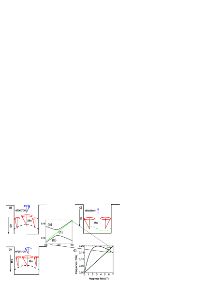
Figure 1: (Color online) Schematic representation of the mean field spin precession modes (a,b) and the long-living mode, where the magnetic ions are decoupled from the carriers (c). Dashed lines map the distribution of the transverse spin component for the magnetic ions. Arrows are the snapshot of the precessing spin vectors of magnetic ions (long arrows shown in the center and at the interfaces) and electron (short arrows). Field dependence of the mode frequencies are shown in (d). The inset enlarges the resonance region.

The spin excitations are identified using all-optical spin resonance technique KikkawaScience . The 100 fs pulses produced by a mode-locked Al₂O₃:Ti laser with a repetition rate of 82 MHz are spectrally filtered to obtain $\sim$1.5 ps pulses tuned to the heavy hole exciton transition. The laser light beam is separated into the pump (200 $\mu$W) and probe (100 $\mu$W) The polarization of the pump is modulated between left and right helicities at 50 kHz, in addition to the intensity modulation of both pump and probe beams. Both beams are focused on the $200$ $\mu$m diameter spot on the surface of the sample. The pump-induced rotation of the linear polarization of the reflected probe (Kerr rotation) is measured as a function of delay between pump and probe pulses. It is usually assumed to be proportional to the spin polarization in the direction of the light. The sample is placed in the cryostat at $T=2$ K under magnetic field $B\sim 6$ T in the plane of the sample (along $z$-axis).

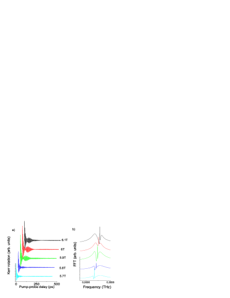
Figure 2: (Color online) Time-resolved Kerr rotation signal under magnetic field from 5.5 T to 6.1 T (a) and the corresponding Fourier spectra (b).

Let us consider what happens when DMS quantum well is excited by the pump pulse. Prior to the excitation the magnetic ions are strongly spin polarized in $z$ direction. Circularly polarized pump pulses create in the quantum well about $10^{10}$ cm^-2 electrons and holes spin polarized normal to the plane, in the $x$-direction. The hole spin is locked in this direction, because the $g$-factor of the hole is vanishing in the direction perpendicular to the quantum well axis. Nevertheless, the hole spin acts on the magnetic ion spins as an effective magnetic field, until the hole spin is fully relaxed ($\tau_{h}\sim$5 ps). It coherently rotates the spins of the magnetic ions away from the $z$-direction and initiates the precession of the Mn spins around the total magnetic field, created by photocreated carriers and the external field CrookerPRL . The electron spin is also expected to precess around the field, created by the hole spins, Mn spins and the external field. Thus, because Kerr rotation signal is proportional to the $x$-component of the magnetization in the sample, we expect to measure the dynamics of the optically generated transverse spin component resulting from the ensemble of the interacting spin subsystems.

Fig.2 shows a set of Kerr rotation measurements under magnetic fields from 5.7 to 6.1 T for the sample 1 (a) and the corresponding Fourier spectra obtained after the fitting procedure (b) notesample1 . We identify in these curves four different components. The first one is the exponential decay of the signal during first $\sim$5 ps after the excitation. It is due to the hole spin relaxation. Two other components are the damped cosines, the corresponding decay times and frequencies strongly vary from 5.7 to 6.1T. The frequencies are plotted as a function of magnetic field in Fig. 3a (circles and squares). One can see a clear anticrossing behavior. These are the collective modes discussed in Refs. Teran ; KonigMD , where precessing electron an Mn spins are strongly coupled. Fig. 3b shows the relaxation times of the collective modes.

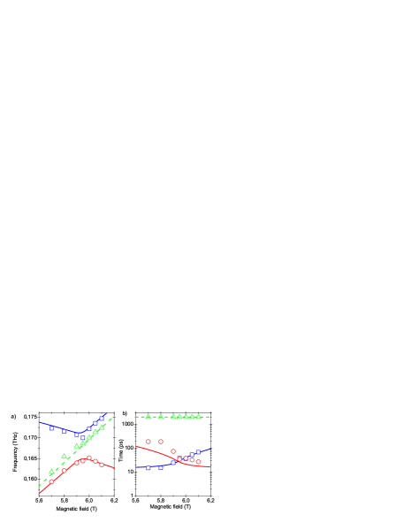
Figure 3: (Color online) Spin precession frequencies (a) and spin coherence times (b) extracted from the data shown in Fig. 2a. Symbols show the experimental data, lines are the the best fit obtained using Eq. (1) assuming electron spin polarization of 70%. Soled lines indicate the collective modes, dashed lines show Mn spin excitations decoupled from electrons.

As it can be expected for the two coupled oscillators with very different quality factors (like electron and magnetic ion spins), the spin relaxation time of the Mn-like mode (circles) is dramatically reduced in the vicinity of the resonance.

However, careful analysis of the data shows that the correct description of the signal imposes taking into account a forth oscillating component (Fig. 2). It is related to another, unexpected spin precession mode. It has the longest relaxation time, which could not be precisely determined, but estimated to be at least of 2000 ps. The field dependence of this long-living mode frequency is linear, and is given by the $g$-factor of 2.02, which corresponds precisely to the Mn spin $g$-factor (Fig. 3, triangles) Crooker , Akimoto . It is unlikely due to the spatial regions in the well where the carriers are absent. Indeed, in both samples the electron gas is strongly degenerate and the electrons are fully delocalized in the plane of the quantum well Cox . The existence of the long-living spin excitations is further corroborated by the resistively detected electron paramagnetic resonance experiments of Ref. Teran , where an additional feature at the Mn spin resonance frequency was detected, though not discussed in the paper.

We develop here the model for the electron gas coupled to the magnetic ions, which allows for the description of both the complex spectrum of the spin excitations in this system and the dephasing of the modes. It is based on the standard Hamiltonian:

$$H=H_{0}+V+g_{e}\mu_{B}\sum_{\beta}(\mathbf{S}_{\beta}\mathbf{B})+g_{m}\mu_{B}\sum_{k}(\mathbf{J}_{k}\mathbf{B})-$$

$${\raggedleft\alpha\sum_{\beta,k}\delta(\mathbf{r}_{\beta}-\mathbf{R}_{k})(\mathbf{S}_{\beta}\mathbf{J}_{k}).~{}~{}~{}~{}~{}~{}~{}~{}~{}~{}~{}~{}\@add@raggedleft}$$ (2)

Here $H_{0}$ defines the kinetic and potential energy of the electrons confined in the quantum well, $V$ is the impurity scattering potential, including the potential of magnetic ions. $\mathbf{S}_{\beta}$, $\mathbf{J}_{k}$ are electron and magnetic ion spin operators, respectively. The $g$-factors of electrons and Mn are $g_{e}=-1.5$ and $g_{m}=2$, respectively, $\mu_{B}$ is the Bohr magneton Sirenko . The last term in the Hamiltonian (2) describes the exchange interaction of the ferromagnetic type between the electrons and Mn spins, $\alpha=1.5\times 10^{-23}$ eV/cm³. Vectors $\mathbf{R}_{k}$ and $\mathbf{r}_{\beta}$ denote the positions of the ions and the electrons, respectively.

We limit our consideration to the strong fields $B\sim 5-6$ T, so that at equilibrium the magnetic ions are almost fully polarized in the direction opposite to the magnetic field and $J_{z}=-5/2$. The polarization of the electrons is mainly determined by the strong exchange field created by the spin polarized ions and thus oriented in the same direction.

Starting from the Hamiltonian (2) we derive the equations of motion for the electron and Mn spin operators and average them over the initial state, where both electron and ion spins are slightly tilted with respect to their orientation at equilibrium. Bearing in mind that the non-equilibrium components of all the spins are small, with respect to their equilibrium components, we linearize the equations of motion about the equilibrium spin values $S_{z}$ and $J_{z}$. In order to simplify the calculations we assume the continuous density of the magnetic ions and replace the summations over their coordinates by the integration according to $\sum_{k}\rightarrow(n_{m}/w)\int d^{3}\mathbf{R}$, where $w$ is the width of the quantum well. This assumption seems reasonable because the concentration of the ions is much larger than the concentration of the electrons, so that a volume defined by the electron de Broglie wavelength contains $\sim 500$ ions. Besides, we suppose that the magnetic ion spins are excited homogeneously in the plane of the sample. We end up with two equations of motion for the average non-equilibrium spin components normalized by the corresponding equilibrium spin values, $\sigma(t)=(S_{x}(t)+iS_{y}(t))/S_{z}$ for electrons and $j(x,t)=(J_{x}(x,t)+iJ_{y}(x,t))/J_{z}$ for magnetic ions. Looking for the solutions in the form $\sigma(t)=\sigma_{0}e^{i\omega t}$ and $j(x,t)=j_{0}(x)e^{i\omega t}$ we obtain the equation on the eigenfrequencies $\omega$ and eigenvectors $(\sigma_{0},j_{0}(x))$:

$$\omega\sigma_{0}=\Omega_{e}\sigma_{0}-\Delta\bar{j}_{0}+i\frac{\sigma_{0}}{\tau_{e}}~{}~{}~{}~{}~{}~{}~{}~{}~{}~{}~{}~{}~{}~{}~{}~{}~{}~{}~{}~{}~{}~{}~{}~{}~{}~{}~{}~{}~{}~{}~{}~{}~{}~{}~{}~{}$$ (3)

$$\omega j_{0}(x)=(\Omega_{m}+K\kappa(x))j_{0}(x)-Kw\chi^{2}(x)\sigma_{0}~{}~{}~{}~{}~{}~{}~{}~{}~{}~{}~{}~{}$$ (4)

where $\chi(x)$ is the electron wavefunction at the lowest quantized state, $\Omega_{e}=g_{e}\mu_{B}B/\hbar+\Delta$, $\Delta=-\alpha n_{m}J_{z}/w\hbar$, $\Omega_{m}=g_{m}\mu_{B}B/\hbar$, $K=-\alpha n_{e}S_{z}/w\hbar$, $\kappa(x)=w\chi^{2}(x)-1$, $\bar{j}_{0}=\int_{0}^{w}\chi^{2}(x)j_{0}(x)dx$ NoteKonigMD . Here we account for the short electron spin relaxation time $\tau_{e}$ by introducing phenomenologically the relaxation term in Eq. (3).

The first terms in the righthand part of the Eqs. (3) and (4) describe the precession of the electron and ion spins. Both corresponding frequencies contain two contributions. The first one comes from the Zeeman effect, while the second accounts for the exchange field created by the equilibrium spin polarization of the ions and electrons, respectively. For electrons, the precession frequency is mainly determined by the exchange field. This field depends on the equilibrium polarization of the ions, which is given by the Brillouin function, saturating at $B\sim 5$ T. Therefore, because $g_{e}<0$ in CdMnTe, the electron spin precession frequency decreases with the magnetic field above $5$ T. In contrast, $x$-dependent exchange contribution in the spin precession of the ions is very small compared to the Zeeman contribution (in our sample three orders of magnitude smaller). While it can be neglected in the eigen frequencies calculation procedure, it appears to be important for the calculation of the relaxation times.

Now it is convenient to come back to the discrete form of Eqs. (3) and (4). The two-dimensional layer decomposes naturally into N components, where N is the number of the atomic layers in the quantum well. Denoting by $x_{n}$ the coordinates of these layers we obtain:

$$\omega\sigma_{0}=\Omega_{e}\sigma_{0}-\Delta\bar{j}_{0}+i\frac{\sigma_{0}}{\tau_{e}}~{}~{}~{}~{}~{}~{}~{}~{}~{}~{}~{}~{}~{}~{}~{}~{}~{}~{}~{}~{}~{}~{}~{}~{}~{}~{}~{}~{}~{}~{}~{}~{}~{}~{}$$ (5)

$$\omega j_{n}=(\Omega_{m}+K\kappa_{n})j_{n}-Kw\chi_{n}^{2}\sigma_{0}~{}~{}~{}~{}~{}~{}~{}~{}~{}~{}~{}~{}~{}~{}~{}~{}~{}~{}~{}~{}~{}~{}~{}~{}$$ (6)

where $\kappa_{n}=\kappa(x_{n})$, $\chi_{n}^{2}=\chi^{2}(x_{n})$, and $\bar{j}_{0}=w/N\sum_{n=1}^{N}\chi_{n}^{2}$. Let us first neglect the small term $K\kappa_{n}$ in the righthand part of the Eq. (6). The resulting equations can be easily solved analytically. They have two solutions for $\sigma_{0}$ and $\bar{j}_{0}$ with frequencies $\omega_{\pm}$ given by (1), where $\omega_{e}=\Omega_{e}+i/\tau_{e}$ and $\omega_{m}=\Omega_{m}$, $\delta^{2}=\eta\Delta K$, $\eta=w\int_{0}^{w}\chi^{4}(x)dx$ infbarr . These are the collective modes discussed in Ref. (Teran ; KonigMD ) noteMD1 . Our model allows also for the estimation of their relaxation times. At resonance the relaxation times of both collective modes are equal $\tau=2\tau_{e}$. The calculated frequencies and the decay times of the collective modes are shown in Fig.3 by solid lines, they are in good agreement with the experimental data. Note, that the spin polarization degree of the electron gas is the only fitting parameter in this calculation ( 70% in sample 1), the electron spin decay time $\tau_{e}=15$ ps being extracted from the fit of the Kerr rotation signal at low magnetic fields, i.e. far from the resonance.

However, the possible spin excitations are not exhausted by the above collective modes. Indeed, in the approximation made above ($K\kappa_{n}\sim 0$) Eqs. (5) and (6) are satisfied if the electron spin is not excited, so that $\sigma_{0}=0$, and at the same time $\bar{j}_{0}=0$ (Fig. 1c). These conditions describe the excitations for which the total exchange field created by the non-equilibrium components of the ion spins are zero, and therefore they do not affect the equilibrium electron spin. The corresponding eigenfrequency $\omega=\Omega_{m}$ fits the experimental results (dashed line in Fig. 3a). The number of such degenerate modes is $N-1$. The relaxation time associated with each of these modes is infinite Mnspinrel , as far as the correction $K\kappa_{n}$ is neglected in Eq. (6).

Let us now take into account the correction $K\kappa_{n}$. The Eqs. (5) and (6) can still be solved analytically. As a result we obtain that the collective modes frequencies $\omega_{\pm}$ and relaxation times are only slightly affected by this term. Its main effect is the lifting of the degeneracy of the N-1 ”everlasting” modes, leading to the broadening of the corresponding spin resonance $\delta\omega\sim K$. One can show, that approximately half of these modes remains decoupled from the electron spin, and therefore does not decay. The remaining modes weakly interact with the electrons and thus acquire a relaxation time of the order of $\tau_{e}\Delta/K$. In our experiments $\tau_{e}\Delta/K>>1/K$. Therefore we expect the decay of the Kerr rotation signal from the long-living spin excitations at the frequency $\Omega_{m}$ after a characteristic time $\tau_{m}\sim 1/K\sim 1$ ns. This is a good order of magnitude (dashed line in Fig.3b), while it is much shorter than any homogeneous relaxation time Konig . Thus, at resonance, Mn spin dephasing due to non-uniform distribution of the electron density in the growth direction appears to be the dominant spin decay mechanism.

Finally, we discuss the possible source of the electron spin relaxation $\tau_{e}\sim$15 ps. This value is considerably shorter than the theoretical predictions Semenov . We suggest, that electron spin dephasing is governed by the fluctuations of the exchange field created by the ions on the scale of the electron wavelength $\lambda$ and, therefore, it is intimately related with the fluctuations of the concentration of the ions on this scale. This effect is missing in the Eqs. (3)-(6), which are written assuming continuous and homogeneous distribution of the ion density. The estimation for our sample leads to $1/\tau_{e}\sim\ (\alpha/\hbar\lambda^{2})\sqrt{n_{m}\lambda^{2}}\sim(\alpha/\hbar)\sqrt{n_{m}n_{e}}\sim 10^{11}$ s^-1 in good agreement with the experimental value. Thus, we assert that the dephasing of both electron and Mn spin excitations is governed by the spatial inhomogeneity of the corresponding exchange fields, and is stronger for the electrons $\tau_{e}<<\tau_{m}$ because their concentration is much smaller than Mn concentration.

In conclusion, we have identified a new kind of spin excitations in DMS quantum wells. These excitations do not involve electrons, which are at equilibrium, while the Mn spins precess as if they were not affected by the exchange interaction. Neither their frequency, nor their relaxation time is affected by the strong exchange interaction with electron spin. The formation of the collective modes discovered by Teran at al Teran is shown to be responsible for the dramatic reduction of the Mn spin relaxation time under resonant conditions. We are able to interpret the ensemble of the experimental observations in the framework of a simple semiclassical model going beyond the mean field approximation.

- (1) J.M. Kikkawa, D.D. Awschalom, Nature 397 139 (1999); G.A. Prinz, Science 282, 1660 (1998)
- (2) F. J. Teran, M. Potemski, D. K. Maude et al, Phys. Rev. Lett 91, 077201 (2003).
- (3) J. König and A. H. MacDonald, Phys. Rev. Lett.91, 077202 (2003).
- (4) V. Huard, R. T. Cox, K. Saminadayar, A. Arnoult, and S. Tatarenko Phys. Rev. Lett. 84, 187 (2000)
- (5) B. König et al Phys. Rev. B 61, 16870 (2000).
- (6) J. M. Kikkawa, D. D. Awschalom, Science 287, 473
- (7) S. A. Crooker, J. J. Baumberg, F. Flack, N. Samarth, D. D. Awschalom, Phys. Rev. Lett. 77, 2814 (1996).
- (8) S. A. Crooker, D. D. Awschalom, J. J. Baumberg, F. Flack, and N. Samarth Phys. Rev. B 56, 7574 (1997).
- (9) R. Akimoto, K. Ando, F. Sasaki, S. Kobayashi, T. Tani, Phys. Rev. B 57, 7208 (1998).
- (10) The results are very similar for the sample 2.
- (11) A. A. Sirenko, T. Ruf, M. Cardona, et al., Physical Review B 56, 2114 (1997).
- (12) These equations can be obtained by the minimization of the affective action calculated in Ref. KonigMD , Eq. (8).
- (13) In the approximation of the infinite barriers the electron wavefuction is and .
- (14) Factor is, however, absent in the expression for from Ref.(KonigMD ) and the role of is played by the average spin of the ions.
- (15) The coherence time of each ”everlasting” mode is anyway limited by the relaxation of the individual Mn spins, mainly on the lattice phonons.
- (16) Y. G. Semenov, Phys. Rev. B 67, 115319 (2003).