From Graph States to Two-Graph States

Abstract

The name ‘graph state’ is used to describe a certain class of pure quantum state which models a physical structure on which one can perform measurement-based quantum computing, and which has a natural graphical description. We present the two-graph state, this being a generalisation of the graph state and a two-graph representation of a stabilizer state. Mathematically, the two-graph state can be viewed as a simultaneous generalisation of a binary linear code and quadratic Boolean function. It describes precisely the coefficients of the pure quantum state vector resulting from the action of a member of the local Clifford group on a graph state, and comprises a graph which encodes the magnitude properties of the state, and a graph encoding its phase properties. This description facilitates a computationally efficient spectral analysis of the graph state with respect to operations from the local Clifford group on the state, as all operations can be realised graphically. By focusing on the so-called local transform group, which is a size 3 cyclic subgroup of the local Clifford group over one qubit, and over $n$ qubits is of size $3^{n}$, we can efficiently compute spectral properties of the graph state.

1 Introduction

1.1 Codes with phase

Consider a binary linear code, ${\cal C}$, of length $n$ and dimension $k$. We can represent ${\cal C}$ by its indicator vector in $({\mathbb{Z}}_{2}^{2})^{\otimes n}$, ${\cal I}_{m}=(m(0\ldots 0),m(0\ldots 1),\ldots,m(1\ldots 1))=(m({\bf{x}}))$, where $m$, the indicator function, is a mapping from ${\mathbb{Z}}_{2}^{n}\rightarrow{\mathbb{Z}}_{2}$ such that $m({\bf{x}})=1$ iff ${\bf{x}}\in{\cal C}$, otherwise $m({\bf{x}})=0$. The indicator vector is, therefore, the truth-table of $m$. For example, the $n=3$, $k=2$ binary linear code, with codewords ${\cal C}=\{000,011,110,101\}$, can be represented by the indicator vector ${\cal I}_{m}=(1,0,0,1,0,1,1,0)$. The indicator function is a Boolean function and respects a non-unique factorization, $m({\bf{x}})=\prod_{i=0}^{n-k-1}m_{i}({\bf{x}})$, where the Boolean functions, $m_{i}$, are affine functions, i.e. of algebraic degree $\leq 1$ if ${\cal C}$ is linear, in which case each function, $m_{i}$, represents the row of a parity-check matrix that defines ${\cal C}$. For instance, for the above example, $m({\bf{x}})=(x_{0}+x_{1}+x_{2}+1)$. As another example, if ${\cal C}=\{010,101\}$, then ${\cal I}_{m}=(0,0,1,0,0,1,0,0)$ and $m$ can be written as $m({\bf{x}})=(x_{0}+x_{1})(x_{0}+x_{2}+1)=(x_{0}+x_{1})(x_{1}+x_{2})=(x_{0}+x_{2}+1)(x_{1}+x_{2})$ where, in this case, ${\cal C}$ is a coset code as it is a binary linear code additively offset by the codeword $010$. By placing the ‘ones’ in different positions in ${\cal I}_{m}$, one can, more generally, represent any binary nonlinear code, where $m$ is no longer the product of affine factors. We do not consider such generalisations in this paper but we do consider another generalisation where a $\pm 1$ phase can be applied to every entry of ${\cal I}_{m}$ - thus we consider codes where every codeword has an associated phase. In order to accomodate such a generalisation we introduce the indicator vector, $\left|\psi\right>=\frac{1}{\sqrt{w(m)}}(m(0\ldots 0)(-1)^{p(0\ldots 0)},m(0\ldots 1)(-1)^{p(0\ldots 1)},\ldots,m(1\ldots 1)(-1)^{p(1\ldots 1)})=(\frac{1}{\sqrt{w(m)}}m({\bf{x}})(-1)^{p({\bf{x}})})$, being a vector in $({\mathbb{C}}^{2})^{\otimes n}$, where $w(m)$ is the support weight of $m$ (i.e. the number of ‘ones’ in the truth-table of $m$), and $m$ and $p$ are Boolean functions from ${\mathbb{Z}}_{2}^{n}\rightarrow{\mathbb{Z}}_{2}$, although we embed the ${\mathbb{Z}}_{2}$ output of $m$ into $\{0,1\}$ of the complex numbers. With such a definition, $\left|\psi\right>$ is normalised such that $\sum_{{\bf{x}}\in{\mathbb{Z}}_{2}^{n}}|\left|\psi\right>_{{\bf{x}}}|^{2}=1$ and the codeword ${\bf{x}}$ can be considered to be sampled from the code, ${\cal C}$, defined by $\left|\psi\right>$, with probability $|\left|\psi\right>_{{\bf{x}}}|^{2}$. In this paper we focus on the case where $m$ is a product of affine Boolean functions and $p$ is a quadratic Boolean function. For example, the $n=3$, $k=2$ binary linear ‘code-with-phase’ comprising codewords ${\cal C}=\{+000,-011,-110,-101\}$, can be represented by the indicator vector $\left|\psi\right>=\frac{1}{2}(1,0,0,-1,0,-1,-1,0)=\frac{1}{2}m(-1)^{p}=\frac{1}{2}(x_{0}+x_{1}+x_{2}+1)(-1)^{x_{0}x_{1}+x_{2}}=\frac{1}{2}(x_{0}+x_{1}+x_{2}+1)(-1)^{x_{1}x_{2}+x_{1}+x_{2}}=\frac{1}{2}(x_{0}+x_{1}+x_{2}+1)(-1)^{x_{0}x_{2}+x_{0}+x_{2}}=\frac{1}{2}(x_{0}+x_{1}+x_{2}+1)(-1)^{x_{0}x_{1}+x_{0}+x_{1}}$. For a given $m$ function, there will, in general, be more than one choice of $p$ function. The choice of letters, $m$ and $p$, is to remind the reader that $m$ assigns ‘magnitude’ to the codewords in the code, and $p$ assigns ‘phase’. Later in this paper we shall need to generalise to indicators of the form $\left|\psi\right>=(\frac{1}{\sqrt{w(m)}}m({\bf{x}})i^{p({\bf{x}})})$ where $m$ is, once again, a product of affine Boolean functions, but now $p$ is a generalised quadratic Boolean function from ${\mathbb{Z}}_{2}^{n}\rightarrow{\mathbb{Z}}_{4}$ of the ‘special form’ $p({\bf{x}})=(\sum_{i<j}a_{ij}x_{i}x_{j})+(\sum_{j}b_{j}x_{j})+c$, were $a_{ij}\in\{0,2\}$, and $b_{j},c\in\{0,1,2,3\}$.

1.2 Quantum states and the local Clifford group

The use of ‘bra-ket’ notation, $\left|*\right>$, to denote the code-with-phase indicator is because $\left|\psi\right>$ can be interpreted as the description for a pure quantum state vector of $n$ qubits with the property that the $n$ qubits described by $\left|\psi\right>$ are projected into state ${\bf{x}}$ with probability $|\left|\psi\right>_{{\bf{x}}}|^{2}$ by a joint measurement of $\left|\psi\right>$ in the so-called ‘computational basis’ [20]. We shall show (corollary 2) that, by restricting $m$ to a product of affine functions, and $p$ to a generalised quadratic Boolean function of the special form described previously, $\left|\psi\right>$ describes, exactly, the class of quantum stabilizer states for qubits [3, 13].

Two pure $n$-qubit states, $\left|\psi^{\prime}\right>$ and $\left|\psi\right>$, are considered locally-equivalent if there exists a $2^{n}\times 2^{n}$ unitary matrix, $U$, with tensor factorisation $U=U^{(0)}\otimes U^{(1)}\otimes\ldots\otimes U^{(n-1)}$, where each $U^{(i)}$ is a $2\times 2$ unitary matrix, such that $\left|\psi^{\prime}\right>=U\left|\psi\right>$. In the context of quantum information, local equivalence preserves the structure of the $n$-partite quantum system, in particular the $n$-partite entanglement of the system [20]. An important group of $2\times 2$ unitary matrices is the (complex) local Clifford group, ${\bf C_{1}}$ which can be generated by the Hadamard matrix, $H=\frac{1}{\sqrt{2}}\tiny\left(\begin{array}[]{rr}1&1\\ 1&-1\end{array}\right)$, and the negahadamard matrix, $N=\frac{1}{\sqrt{2}}\tiny\left(\begin{array}[]{rr}1&i\\ 1&-i\end{array}\right)$, where $i=\sqrt{-1}$. The $n$-qubit local Clifford group is then given by ${\bf C_{n}}={\bf C_{1}}^{\otimes n}$. A graph state is of the form $\left|\psi\right>=2^{\frac{-n}{2}}(-1)^{p}$, where $p$ is a homogeneous quadratic Boolean function and, implicitly, $m=1$. When $m=1$, all $\left|\psi\right>_{\bf x}$ have the same magnitude, and we refer to such state vectors, $\left|\psi\right>$, as flat [28]. The homogeneous quadratic, $p$, maps, bijectively, to a simple graph [30]. It can be shown that every stabilizer state is locally equivalent to a set of graph states, where each such graph state is obtained via the action of a specific unitary from ${\bf C_{n}}$ on the stabilizer. In this paper we represent stabilizer states by the form $\left|\psi\right>=2^{\frac{-n}{2}}mi^{p}$, where $p$ is quadratic of the special form and $m$ is a product of affine Boolean functions [22]. This form is a generalisation of that for a graph state. As $m$ is the indicator function for a binary linear coset code, it can be represented by a bipartite graph with loops, as will be made clear later [22, 9]. As both $m$ and $p$ can, with minor embellishments, be represented by graphs, we refer to $\left|\psi\right>$ of this form as a two-graph state and the two-graph state is a bi-graphical representation of a stabilizer state.

1.3 The Pauli group, stabilizer states, and graph states

The single-qubit Pauli group of matrices, ${\bf P_{1}}$, is generated by $X=\tiny\left(\begin{array}[]{rr}0&1\\ 1&0\end{array}\right)$, $Z=\tiny\left(\begin{array}[]{rr}1&0\\ 0&-1\end{array}\right)$, and $i$, and the Pauli group for $n$ qubits is ${\bf P_{n}}={\bf P_{1}}^{\otimes n}$. Formally, a stabilizer state over a system of $n$ qubits is defined to be a joint eigenvector of a stabilizer generated by a certain subgroup of ${\bf P_{n}}$ [3, 13, 4]. A graph state is a special case of a stabilizer state, being a joint eigenvector of a subgroup of ${\bf P_{n}}$, and the graph state can be described by the edges of a simple graph with $n$ nodes [25, 32, 17]. The stabilizer generated by a subgroup of the Pauli group came to prominence in the mid-90’s when it was used to describe a class of quantum error-correcting codes [3, 13]. In this context the stabilizer state describes a quantum error-correcting code of zero dimension which is robust to errors caused by a convex combination of members of the Pauli group.

It has been shown in [28, 35] that the graph state can always be represented by a homogeneous quadratic Boolean function whose structure can be bijectively mapped to the associated graph in an obvious way. Although the graph state has its origins in the theory of eigensystems, its re-interpretation as a quadratic Boolean function allows one to consider new cryptographic criteria for the function, such as its generalised bentness [28, 30], or aperiodic propagation criteria [6], and to justify applying such criteria to Boolean functions of higher degree. In this paper we express the stabilizer state as a two-graph state, this being a simultaneous generalisation of a binary linear coset code and a quadratic Boolean function. Such a generalisation shall allow us, in future work, to propose and investigate new criteria for binary linear codes, and also to establish unforeseen links between Boolean functions and coding theory. Stabilizer states also have a natural interpretation as GF$(4)$ additive codes [3] and the analysis of graph states relates naturally to recent graph-theoretic results for the associated graphs [27].

1.4 The action of the local Clifford group

Apart from highlighting the two-graph, magnitude-phase form of the stabilizer state, the primary purpose of this paper is to efficiently describe how the action of unitary matrices from the local Clifford group, ${\bf C_{n}}$, modify the form of the two-graph state. In particular, we focus on efficiently computing spectral metrics of the form $\sum_{U\in{\bf C_{n}}}\sum_{\bf{x}}|U\left|\psi\right>_{\bf{x}}|^{j}$ for some integer $j$. In such cases one is only interested in the magnitudes of the elements of $U\left|\psi\right>$, not their phases, and this simplification allows us to further simplify as we only need to sum over all $U$ in a size $3^{n}$ subgroup, ${\bf T_{n}}$, of the local Clifford group, as shall be explained later. It has been shown in previous work [1, 4, 8, 9, 11, 28, 29, 30, 35, 36] how the action of matrices from the local Clifford group on the graph state can be realised using only local graphical operations, where linear phase offsets, generated by each matrix action, are repeatedly eliminated by invoking local equivalence. These two graphical operations are called edge-local complementation (ELC) (sometimes called pivot), and local complementation (LC), where ELC can be decomposed into a series of LCs. Whilst ELC acting on bipartite graphs can be used to classify binary linear codes [9], LC acting on graphs can be used to classify additive codes over GF$(4)$ [4]. In this paper, ELC and LC are generalised so as to realise the action of matrices from the local Clifford group on the two-graph state, without the requirement to repeatedly eliminate linear phase offsets.

1.5 Example

Here is a small example that should clarify some of the ideas discussed so far:

Consider the $n=3$-qubit graph state, $\left|\psi\right>$, which is the joint eigenvector of the group of commuting operators, $\langle{\cal{K}}_{0},{\cal{K}}_{1},{\cal{K}}_{2}\rangle$, where ${\cal{K}}_{0}=X\otimes Z\otimes I$, ${\cal{K}}_{1}=Z\otimes X\otimes Z$, ${\cal{K}}_{2}=I\otimes Z\otimes X$, and $I$ is the $2\times 2$ identity matrix. Then $\left|\psi\right>$ can be represented by the simple graph, $P=({\cal V}_{P},{\cal E}_{P})$, with vertices ${\cal V}_{P}=\{0,1,2\}$ and edges ${\cal E}_{P}=\{01,12\}$. The state $\left|\psi\right>$ can be written explicitly in the computational basis as $\frac{1}{\sqrt{8}}(\left|000\right>+\left|001\right>+\left|010\right>-\left|011\right>+\left|100\right>+\left|101\right>-\left|110\right>+\left|111\right>)$, which we abbreviate to $\left|\psi\right>=\frac{1}{\sqrt{8}}(1,1,1,-1,1,1,-1,1)$, and can alternatively be written, using algebraic normal form (ANF) for the phase, as $\left|\psi\right>=(\frac{1}{\sqrt{8}}(-1)^{p({\bf{x}})})=(\frac{1}{\sqrt{8}}(-1)^{x_{0}x_{1}+x_{1}x_{2}})$, where $p:{\mathbb{Z}}_{2}^{3}\rightarrow{\mathbb{Z}}_{2}$ , and $\left|\psi\right>_{\bf x}=\frac{1}{\sqrt{8}}(-1)^{p({\bf{x}})}$. The quadratic monomial $x_{i}x_{j}$ is a term in $p$ iff $ij$ is an edge in $P$. Let $\left|\psi^{\prime}\right>=(I\otimes N\otimes I)\left|\psi\right>=\frac{\omega}{\sqrt{8}}(-1)^{x_{0}x_{1}+x_{0}x_{2}+x_{1}x_{2}}i^{3(x_{0}+x_{1}+x_{2})}$, where $i=\sqrt{-1}$, and $\omega=e^{\pi i/4}$. Then $\left|\psi^{\prime}\right>$ is flat, and the quadratic part of $\left|\psi^{\prime}\right>$ represents the graph $P^{\prime}$ with edge set ${\cal{E}}_{P^{\prime}}=\{01,02,12\}$ - the affine part of $\left|\psi^{\prime}\right>$ can be eliminated by subsequent action of the diagonal unitary, $D=\omega^{7}\tiny\left(\begin{array}[]{rr}1&0\\ 0&i\end{array}\right)\otimes\left(\begin{array}[]{rr}1&0\\ 0&i\end{array}\right)\otimes\left(\begin{array}[]{rr}1&0\\ 0&i\end{array}\right)$, which is in ${\bf C_{n}}$. The state, $\left|\psi^{\prime}\right>$ is, by construction, local unitary equivalent, via unitaries from ${\bf C_{n}}$, to the graph state $\left|\psi\right>$, and therefore represents, to within local equivalence, the same stabilizer state as $\left|\psi\right>$. A graphical way of interpreting the action of $D(I\otimes N\otimes I)$ on $\left|\psi\right>$ is to perform the action of local complementation on $P$ at vertex $1$ to produce graph $P^{\prime}$, that is to complement all edges between the neighbours of vertex $1$. This example shows how the action of a unitary from the local Clifford group maps between two locally-equivalent graph states. But, let us now consider $\left|\psi^{\prime\prime}\right>=(H\otimes I\otimes I)\left|\psi\right>=\frac{1}{2}(1,0,0,1,1,0,0,-1)$, which, by construction, is the same stabilizer state as $\left|\psi\right>$, to within local equivalence, but not a graph state as we cannot represent $\left|\psi^{\prime\prime}\right>$ using only a quadratic Boolean function for its phase part. But we can represent $\left|\psi^{\prime\prime}\right>$ using a two-ANF representation:

$$\left|\psi^{\prime\prime}\right>=\frac{1}{2}m^{\prime\prime}({\bf{x}})(-1)^{p^{\prime\prime}({\bf{x}})}=\frac{1}{2}(x_{0}+x_{1}+1)(-1)^{x_{1}x_{2}},$$

where $\left|\psi^{\prime\prime}\right>_{\bf{x}}=m^{\prime\prime}({\bf{x}})(-1)^{p^{\prime\prime}({\bf{x}})}$, $m^{\prime\prime}:{\mathbb{Z}}_{2}^{2}\rightarrow{\mathbb{Z}}_{2}$, and $p^{\prime\prime}:{\mathbb{Z}}_{2}^{2}\rightarrow{\mathbb{Z}}_{2}$. As mentioned previously, throughout this paper we perform a final embedding of the output of $m$, namely ${\mathbb{Z}}_{2}$, into the complex, $\{0,1\}$, so as to interpret the two-ANF state as a pure quantum state. To keep notation simple, we shall not formally indicate this embedding. We refer to this two-ANF representation as an algebraic polar form (APF) and represent the two ANFs by two graphs, where the polynomials, $m^{\prime\prime}$ and $p^{\prime\prime}$, can be written as magnitude and phase graphs, respectively. $p^{\prime\prime}$ maps to the phase graph $P^{\prime\prime}$ with vertex and edge sets ${\cal{V}}_{P^{\prime\prime}}=\{1,2\}$ and ${\cal{E}}_{P^{\prime\prime}}=\{12\}$, respectively, and $m^{\prime\prime}$ maps to the magnitude graph $M^{\prime\prime}$ with vertex and edge sets ${\cal{V}}_{M^{\prime\prime}}=\{0,1\}$ and ${\cal{E}}_{M^{\prime\prime}}=\{01\}$, respectively. The method of mapping a magnitude polynomial, $m({\bf{x}})$ to its associated magnitude graph, $M$, is explained in definition 9. Although we are conceptually dealing with a two-graph object, $(M,P)$, we prefer to act on an associated single graph, $G$, where the vertex and edge sets of $G$ satisfy ${\cal{V}}={\cal{V}}_{M}\cup{\cal{V}}_{P}$, ${\cal{E}}={\cal{E}}_{M}\cup{\cal{E}}_{P}$, respectively. If we further bipartition the vertex set ${\cal{V}}$ into ${\cal{L}}$ and ${\cal{R}}$, where ${\cal{V}}={\cal{L}}\cup{\cal{R}}$, ${\cal{L}}\cap{\cal{R}}=\emptyset$, and ${\cal{R}}={\cal{V}}_{P}$, then we can exactly recover the graph pair, $(M,P)$, from the graph-set pair, $(G,{\cal{R}})$, so the graph pair and graph-set pair definitions are equivalent.

1.6 Local equivalence and a subgroup of the local Clifford group

Measurement-based quantum computing using cluster states [26] or, more generally, graph states, considers the action of unitary matrices on the graph state, along with measurement of its vertices and classical communication between its vertices. Of particular importance are the action of those unitaries from ${\bf{C_{n}}}$ on the graph state [26]. A classification of the equivalence classes of graph states, wrt unitaries from ${\bf{C_{n}}}$, has been undertaken [18, 16, 8, 5, 12], and, until very recently, it was an open problem to prove that such equivalence classes remain the same even when one widens the class of unitaries considered to include local unitaries outside the local Clifford group [33]. Recent results have, however, suggested that this so-called ‘LU$=$LC conjecture’ is false [15, 19]. Equivalence of graph states wrt the action of unitaries from ${\bf{C_{n}}}$ can be realised on the associated graphs by means of local complementation [1, 2, 11, 35, 4]. In [28] it was shown that successive local complementations on a graph can be realised by considering the action on the graph state of only a small subgroup, ${\bf{T_{n}}}$, of matrices from ${\bf{C_{n}}}$, where ${\bf{T_{n}}}={\bf{T_{1}}}^{\otimes n}$ and ${\bf{T_{1}}}=\{I,\lambda,\lambda^{2}\}$ is a cyclic subgroup generated by $\lambda=\frac{\omega^{5}}{\sqrt{2}}\tiny\left(\begin{array}[]{rr}1&i\\ 1&-i\end{array}\right)$, where ${\bf{T_{1}}}\subset{\bf{C_{1}}}$, and $|{\bf{T_{1}}}|=3$. We call ${\bf{T_{n}}}$ the local transform group over $n$ qubits. Moreover ${\bf{C_{1}}}={\bf{T_{1}}}\times{\bf{D_{1}}}$, where $|{\bf{C_{1}}}|=192$ and $|{\bf{D_{1}}}|=64$, and ${\bf{D_{1}}}$ is a subgroup of diagonal and antidiagonal $2\times 2$ matrices generated by $\omega$, $\tiny\left(\begin{array}[]{rr}1&0\\ 0&i\end{array}\right)$, and $\tiny\left(\begin{array}[]{rr}0&1\\ 1&0\end{array}\right)$. In [28] we concentrate only on the subset of transforms from ${\bf{T_{n}}}$ whose action on a graph state yield flat spectra, where these flat spectra can be interpreted, to within a final multiplication ny a member of ${\bf D_{n}}$, as a set of locally-equivalent graph states. In this paper we, more generally, consider the action of all $3^{n}$ transforms from ${\bf{T_{n}}}$ on a graph state. We show that a graph state is always locally equivalent, wrt unitaries from ${\bf C_{n}}$, to a two-graph object, $(M,P)$, where $M$ and $P$ represent magnitude and phase graphs for the state, respectively, and the action of any member of ${\bf{T_{n}}}$ on such a state can be expressed as a graphical operation on the combined graph formed by $M$ and $P$, to yield another graph which can, once again, be split into a two-graph, $(M^{\prime},P^{\prime})$ object.

To compute the two-graph orbit and/or perform spectral analysis of a certain graph or stabilizer state, neither [28] or this paper use ${\bf{T_{1}}}$ explicitly. Instead we use the set of three matrices, $\{I,H,N\}$. It is evident that $\lambda=\omega^{5}N$, and $\lambda^{2}=\omega^{3}\tiny\left(\begin{array}[]{rr}1&0\\ 0&-i\end{array}\right)H$, so one can always obtain the action of any unitary from the transform group, ${\bf{T_{n}}}$, by first applying the appropriate unitary from $\{I,H,N\}^{\otimes n}$, then applying a suitable unitary from ${\bf{D_{n}}}$, where $\{U_{0},U_{1},\ldots,U_{t-1}\}^{\otimes n}$ means the set of matrices formed by any $n$-fold tensor product of matrices from the set $\{U_{0},U_{1},\ldots,U_{t-1}\}$. But the application of any unitary from ${\bf{D_{n}}}$ to a state does not change coefficient magnitudes. So, to perform spectral analysis based on magnitude computations, we can use $\{I,H,N\}$ instead of ${\bf{T_{1}}}=\{I,\lambda,\lambda^{2}\}$. We choose to do this because $H$ is the 2-point periodic discrete Fourier transform (DFT), and $N$ is the 2-point negaperiodic DFT, and using this viewpoint facilitates a ‘Fourier’ approach to the analysis of graph states and stabilizer (two-graph) states. However, all results in this paper wrt $\{I,H,N\}^{\otimes n}$ are trivially translated into results wrt ${\bf{T_{n}}}$, as shown in subsection 4.1.

1.7 Main aims of this paper

In previous work the use of graphs to represent graph states has simplified both theoretical and computational analyses of graph states. Our primary aim, in this paper, is to use two-graph states to represent stabilizer states, so as to simplify analysis of the stabilizer state, where the graph state is a special case of the two-graph state. We obtain computationally efficient algorithms for the spectral analysis of the graph and two-graph state wrt ${\bf{C_{n}}}$, as the set of spectra computed via the action of $\{I,H,N\}^{\otimes n}$ on a two-graph state acts as a precise summary of the much larger set of spectra resulting from the action of any member of ${\bf{C_{n}}}$ on the two-graph state, where the action of ${\bf{D_{n}}}$ has been factored out. A secondary aim of this paper is to provide an efficient, localised, graphical method to realise the action of any member of ${\bf{C_{n}}}$ on the graph or two-graph state. This is made possible because $H$ and $N$ are generators of ${\bf{C_{1}}}$ and, in this paper, we characterise the actions of $H$ and $N$ on the two-graph state and, therefore, ${\bf{C_{n}}}$ is covered via repeated actions of $H$ and $N$. Moreover, as ${\bf C_{n}}={\bf D_{n}}\times{\bf T_{n}}$, and ${\bf T_{n}}=D\{I,H,N\}^{\otimes n}$, $D\in{\bf D_{n}}$ then, to within a final action by a member of ${\bf{D_{n}}}$, the graphical characterisation of the action of any unitary from $\{I,H,N\}^{\otimes n}$ on a two-graph object, $(G,{\cal{R}})\equiv(M,P)$ will, at the same time, graphically characterise the action of successive unitaries from $\{I,H,N\}^{\otimes n}$ on $(G,{\cal{R}})$.

Section 2 onwards of this paper makes precise the discussion of this introduction. Let $U_{v}=I^{\otimes v}\otimes U\otimes I^{\otimes n-v-1}$. Then it is shown that

• Two-Graph State: The two-graph state comprises a graph with loops, $G$, and a set ${\cal{R}}$ or, equivalently, two graphs $M$ and $P$ ($(G,{\cal{R}})\equiv(M,P)$), and is represented by $m(-1)^{p}$, where $m$ is a product of affine Boolean functions, and $p$ is a quadratic Boolean function, The transition between two representations of the same two-graph state is characterised via the operation called ‘swp’ which operates on $(G,{\cal{R}})$. Then the action of a unitary, $H_{v}$, $v\in{\cal{V}}$, on $(G,{\cal{R}})$ is characterised via the conditional action of ‘swp’ on $(G,{\cal{R}})$, and a set operation on ${\cal{R}}$, to produce another two-graph state, $(G^{\prime},{\cal{R}}^{\prime})\equiv(M^{\prime},P^{\prime})$. Consequently the action of any transform from $\{I,H\}^{\otimes n}$ on a two-graph state can be computed graphically plus a few set operations.

• Generalised Two-Graph State: The generalised two-graph state comprises a graph with loops, $G$, and two sets ${\cal{R}}$ and ${\cal{Q}}$ or, alternatively, two graphs $M$ and $P$ and a set ${\cal{Q}}$, ($(G,{\cal{R}},{\cal{Q}})\equiv(M,P,{\cal{Q}})$), and is represented by $mi^{p}$, where $m$ is a product of affine Boolean functions, and $p$ is a quadratic function from ${\mathbb{Z}}_{2}^{n}\rightarrow{\mathbb{Z}}_{4}$ of the special form. The possible loops at vertices in ${\cal{R}}$ are weighted according to elements in ${\cal Q}$. The transition between two representations of the same generalised two-graph state is characterised via the generalised operation called ‘swp’ which now operates on $(G,{\cal{R}},{\cal{Q}})$. Then the actions of unitaries, $H_{v}$ and $N_{v}$, $v\in{\cal{V}}$, on $(G,{\cal{R}},{\cal{Q}})$ can be characterised via the conditional action of ‘swp’ on $(G,{\cal{R}},{\cal{Q}})$, and certain other conditional operations on $G$,${\cal{R}}$, and ${\cal{Q}}$, to produce another generalised two-graph state, $(G^{\prime},{\cal{R}}^{\prime},{\cal{Q}}^{\prime})\equiv(M^{\prime},P^{\prime},{\cal{Q}}^{\prime})$. Consequently the action of any transform from $\{I,H,N\}^{\otimes n}$ on a generalised two-graph state can be computed graphically plus a few set operations.

• Spectral Analysis of the Graph State: By considering $L_{j}$ norms of the graph state wrt the local Clifford group, we demonstrate the usefulness of the generalised two-graph representation to compute, efficiently, these norms.

We also generalise the graph operations of edge-local complementation (ELC) [27, 36, 9] and local complementation (LC) [1, 2, 11, 35, 4] to the two-graph operations, edge-local complementation^⊙ (ELC^⊙) and local complementation^⊙ (LC^⊙) which now take into account graph loops.

A recent paper [10], independent to ours, also extends the graphical notation to deal with the action of the local Clifford group on stabilizer states. [10] also implicitly utilises a bipartite splitting of the graph (via ‘hollow’ and ‘filled-in’ nodes), and also requires graph loops. [10] describes the action of $H$, $S$ and $Z$ on their graph, whereas we describe the action of $H$ and $N$. Their model and our model must be equivalent in terms of characterising the action of the local Clifford group on stabilizer states. However one can list some differences in approach between the papers as follows. Firstly, [10] focusses, primarily, on modelling the action of the local Clifford group. In contrast, we focus, primarily, on modelling the action of the local transform group, ${\bf T_{n}}$, and/or $\{I,H,N\}^{\otimes n}$ as we are more interested in evaluating spectral metrics for the graph state as efficiently as possible, up to as many qubits as possible, although a secondary result of our work is that the action of the complete local Clifford group is also modelled. Secondly, [10] implicitly considers the stabilizer state as a joint eigenstate, and does not therefore have to consider an explicit basis for the state. In contrast, in our paper we consider an explicit computational basis for the state, and this allows us to distinguish between magnitude and phase properties of the stabilizer state. This, in turn, allows us to evaluate spectral metrics, associated with the graph state, with small effort. Thirdly, by distinguishing between magnitude and phase, we highlight the stabilizer state as a simultaneous generalisation of both the usual classical cryptographic representation of Boolean functions (the phase part), and the usual parity-check graph (factor graph) representation of classical binary linear codes (the magnitude part). The link to parity-check graphs was investigated in [21] and the interaction between magnitude and phase graphs was investigated in [22] and has since been exploited in [23, 28, 29, 4, 6, 7, 8]. A preliminary version of this paper was presented at [31].

For the rest of this paper we only consider connected graph states as, otherwise, the system is degenerate. We also ignore the global multiplicative constants in front of the state vector. In particular our method strictly only distinguishes between the action on the two-graph state of matrices from the size $24^{n}$ subgroup of the local Clifford group, as the supplementary multiplication of the state by a power of $\omega$ is ignored, i.e we remove the centre of the local Clifford group. For most scenarios this global multiplicative constant can be ignored, however a trivial refinement of our method would be necessary if one was to relate the action of the same sequence of matrices from the local Clifford group on two or more two-graph states.

2 Formal Definitions

Define $U_{v}=I^{\otimes v}\otimes U\otimes I^{\otimes n-v-1}$.

Definition 1

Let $I=\tiny\left(\begin{array}[]{cc}1&0\\ 0&1\end{array}\right)$, $H=\frac{1}{\sqrt{2}}\tiny\left(\begin{array}[]{cc}1&1\\ 1&-1\end{array}\right)$, and $N=\frac{1}{\sqrt{2}}\tiny\left(\begin{array}[]{cc}1&i\\ 1&-i\end{array}\right)$ be the $2\times 2$ identity, Walsh-Hadamard, and negahadamard [23] matrices, respectively. The set of $3^{n}$ transforms, $\{I,H,N\}^{\otimes n}$, is defined as the set of all $n$-fold tensor product combinations of matrices $I,\,H$ and $N$.

Definition 2

[22] A pure $n$-qubit state, $\left|\psi\right>=(\left|\psi\right>_{0\ldots 00},\left|\psi\right>_{0\ldots 01},\ldots,\left|\psi\right>_{1\ldots 11})$, with vector entries satisfying $\left|\psi\right>_{\bf{x}}\in c\{0,1,-1\}$, for some complex constant, $c$, can always be written in the form

$$\left|\psi\right>=cm({\bf x})(-1)^{p({\bf x})},$$

where $\left|\psi\right>_{\bf{x}}=cm({\bf x})(-1)^{p({\bf x})}$, $\forall{\bf{x}}\in{\mathbb{Z}}_{2}^{n}$, and $m,p:{\mathbb{Z}}_{2}^{n}\rightarrow{\mathbb{Z}}_{2}$ are both Boolean functions. The output of $m$ is embedded in the complex numbers. We separate, thus, magnitude, $m$, and phase, $p$, of $\left|\psi\right>$, and call such a representation the algebraic polar form (APF) of $\left|\psi\right>$.

Remark: In order to simplify notation we henceforth omit the normalisation constant, $c$, from any expression of the form $\left|\psi\right>=cm({\bf x})(-1)^{p({\bf x})}$ or similar.

Definition 3

Let $G=({\cal{V}},{\cal{E}})$ be a graph with vertex set, ${\cal{V}}$, and edge set, ${\cal{E}}$, where $G$ may contain loops. Let $\Gamma_{G}$ be the binary adjacency matrix of $G$. Then, for two graphs, $G$ and $G^{\prime}$, both defined over the same $n$ vertices, $G^{\prime\prime}=G\pm G^{\prime}$ means that the adjacency matrix, $\Gamma_{G^{\prime\prime}}$, of $G^{\prime\prime}$, satisfies $\Gamma_{G^{\prime\prime}}=\Gamma_{G}\pm\Gamma_{G^{\prime}}$. Let ${\cal{N}}_{v}^{G}$ be the set of vertices other than $v$ which are neighbours of vertex $v$ in $G$. Let ${\cal{B}}_{v}^{G}={\cal{N}}_{v}^{G}\cup\{v\}$ be the set of vertices less than or equal to one edge distance from vertex $v$ in $G$. For a vertex set, ${\cal{V}}$, let $G_{\cal{V}}$ be the induced subgraph of $G$ on ${\cal{V}}$, comprising all edges from $G$ whose endpoints are both in ${\cal{V}}$. For vertex sets, ${\cal{V}}$ and ${\cal{V}}^{\prime}$, define $K_{{\cal{V}},{\cal{V}}^{\prime}}$ to be the graph with binary adjacency matrix, $\Gamma_{K}$, where $\Gamma_{K_{ij}}=\Gamma_{K_{ji}}=1$ iff $i\in{\cal{V}}\setminus{\cal{V}}^{\prime},j\in{\cal{V}}^{\prime}$ or $i=j\in{\cal{V}}\cap{\cal{V}}^{\prime}$. $G_{\cal{V}}$ and $K_{{\cal{V}},{\cal{V}}^{\prime}}$ may contain loops. Let $G_{v}=K_{\{v\},{\cal{N}}_{v}^{G}}$. Let $\Delta_{\cal{V}}$ be the graph with diagonal binary adjacency matrix, $\Gamma_{\Delta}$, where $\Gamma_{\Delta_{ij}}=1$ iff $i=j\in{\cal{V}}$. The complete graph, $C_{{\cal{V}}}$, is the simple graph whose edge set comprises the set of edges $\{vw,\hskip 5.69054pt\mbox{ }\forall v,w\in{\cal{V}},v<w\}$.

Definition 4

[1, 2, 11, 35, 4] The action of local complementation (LC) on a simple graph $G$ at vertex $v$ is the graph transformation obtained by replacing the subgraph $G_{{\cal{N}}_{v}^{G}}$ by its complement.

Example: The action of LC on a graph at vertex $v=0$, is shown in figure 1.

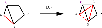
Figure 1: The action of LC at vertex $0$

Definition 5

[27, 36, 9] The action of edge local complementation (ELC) on a simple graph $G$ at edge $vw$ is the graph transformation obtained by performing LC at vertex $v$, then vertex $w$, then vertex $v$ again (or, equivalently, at $w$, then $v$, then $w$ again).

In this paper we generalise both LC and ELC so as to operate on a two-graph object.

Definition 6

Let $G$ be a graph with possible loops, containing an edge $vw$, $v\neq w$. Then $G^{vw}$ is the graph resulting from the action of edge local complementation^⊙ (ELC^⊙) on edge $vw$ of $G$, where

$$G^{vw}=G+K_{{\cal{B}}_{v}^{G},{\cal{B}}_{w}^{G}}+\Delta_{\{v,w\}}+\Gamma_{G_{vv}}\Delta_{{\cal{B}}_{w}^{G}}+\Gamma_{G_{ww}}\Delta_{{\cal{B}}_{v}^{G}}\enspace.$$

Example: The action of ELC^⊙ on the following graph at edge $vw=31$, is shown in figure 2.

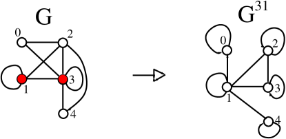
Figure 2: The action of ELC^⊙ at edge $31$

Remark: From definition 6, even when $G$ is a simple graph, $\Gamma_{G_{vv}}=\Gamma_{G_{ww}}=0$, we see that possible loops can still be produced from term $K_{{\cal{B}}_{v}^{G},{\cal{B}}_{w}^{G}}$. The ELC operation, which acts only on simple graphs, can be recovered from ELC^⊙ by applying ELC^⊙ to a simple graph, then deleting any resultant loops from the output.

The Pauli matrix group is generated by $X=\tiny\left(\begin{array}[]{rr}0&1\\ 1&0\end{array}\right)$, $Z=\tiny\left(\begin{array}[]{rr}1&0\\ 0&-1\end{array}\right)$, and $i$. Let $S=\tiny\left(\begin{array}[]{rr}1&0\\ 0&i\end{array}\right)$.

Definition 7

The local Clifford matrix group, ${\bf{C_{1}}}$, is the group of 192 $2\times 2$ matrices that normalise the Pauli group, and can be decomposed as ${\bf{C_{1}}}={\bf{D_{1}}}\times{\bf{T_{1}}}$ where we call ${\bf{D_{1}}}$ the diagonal group and ${\bf{T_{1}}}$ the transform group. ${\bf{T_{1}}}=\{I,\lambda,\lambda^{2}\}$ is a cyclic subgroup generated by $\lambda=\omega^{5}N$, where $i=\sqrt{-1}$ and $\omega=\sqrt{i}$, ${\bf{D_{1}}}={\bf{C_{1}}}/{\bf{T_{1}}}=\left<S,X,\omega\right>$, and comprises only diagonal or antidiagonal $2\times 2$ matrices, and $|{\bf{C_{1}}}|=192$, $|{\bf{T_{1}}}|=3$, and $|{\bf{D_{1}}}|=64$. We call ${\bf{C_{n}}}$, ${\bf{T_{n}}}$, and ${\bf{D_{n}}}$, the groups formed by $n$-fold tensor products of matrices from ${\bf{C_{1}}}$, ${\bf{T_{1}}}$, and ${\bf{D_{1}}}$, respectively, where $|{\bf C_{n}}|=8\times 24^{n}$ and $|{\bf D_{n}}|=8\times 8^{n}$.

Observe that $\lambda=\omega^{5}N$ and $\lambda^{2}=\omega^{3}S^{-1}H$ so, for any $U\in{\bf{T_{n}}}$, and any $V\in\{I,H,N\}^{\otimes n}$, we have $U=\omega DV$ for some $D\in{\bf{D_{n}}}$. For the rest of the paper we focus on the action of $\{I,H,N\}^{\otimes n}$ on the graph state and, more generally, on the two-graph state, where the alternative action of ${\bf{T_{n}}}$ on the state can be derived easily (see section 4.1).

Definition 8

[25] Given a graph, $P$, on $n$ vertices with adjacency matrix, $\Gamma_{P}$, define $n$ commuting Pauli operators

$${\cal{K}}_{P_{j}}=X_{j}\prod_{k\in{\cal{N}}_{j}}Z_{k}=X_{j}\prod_{k=0}^{n-1}Z_{k}^{\Gamma_{P_{jk}}},$$

where ${\cal{N}}_{j}$ is the set of vertices in $P$ that are neighbours of vertex $j$. The stabilizer, ${\cal{K}}_{P}$, is generated by $\langle{\cal{K}}_{P_{0}},{\cal{K}}_{P_{1}},\ldots,{\cal{K}}_{P_{n-1}}\rangle$, and $\left|\psi\right>$ is a graph state iff ${\cal{K}}_{P}\left|\psi\right>=\left|\psi\right>$, for some simple graph, $P$. Explicitly, in the computational basis, [28, 35],

$$\left|\psi\right>_{\bf x}=(-1)^{\sum_{i<j}\Gamma_{P_{ij}}x_{i}x_{j}}.$$

Any state $\left|\psi\right>^{\prime}=U\left|\psi\right>$, $U\in{\bf{C_{n}}}$, is a stabilizer state locally equivalent to $\left|\psi\right>$.

3 The Two-Graph State

Definition 9

A two-graph state is a pure quantum state, $\left|\psi\right>$, of $n$ qubits that can be defined by a graph, $G=({\cal{V}},{\cal{E}})$, and a bipartition, $({\cal{L}},{\cal{R}})$, where ${\cal{V}}={\cal{L}}\cup{\cal{R}}$ and ${\cal{L}}\cap{\cal{R}}=\emptyset$, and where $G_{\cal{L}}$ is the empty graph apart from possible loops. The pair, $(G,{\cal{R}})$, explicitly encodes a two-graph object, $(M,P)$, where $P=G_{\cal{R}}$, and $M=G-P$ is a bipartite graph. The state, $\left|\psi\right>$, is defined by its algebraic polar form, $\left|\psi\right>=cm({\bf{x}})(-1)^{p({\bf{x}})}$, where $c\in{\mathbb{C}}$, $m({\bf{x}}):{\mathbb{Z}}_{2}^{n}\rightarrow{\mathbb{Z}}_{2}$ is a product of affine functions of the form,

$$m({\bf{x}})=\prod_{i\in{\cal{L}}}(\Gamma_{M_{ii}}+1+x_{i}+\sum_{j\in{\cal{R}}}\Gamma_{M_{ij}}x_{j}),$$

such that $m=1$ when ${\cal{L}}=\emptyset$, and where $p({\bf{x}}):{\mathbb{Z}}_{2}^{n}\rightarrow{\mathbb{Z}}_{2}$ is a quadratic function of the form,

$$p({\bf{x}})=\sum_{i,j\in{\cal{R}},i<j}\Gamma_{P_{ij}}x_{i}x_{j}+\sum_{j\in{\cal{R}}}\Gamma_{P_{jj}}x_{j}.$$

Remark: For $(G,{\cal{R}})\equiv(M,P)$ a two-graph state, $M$ and $P$ cannot contain loops at vertices in ${\cal{R}}$ and ${\cal{L}}$, respectively. Also, although at first it seems that we don’t distinguish between for instance $m=(x_{0}+x_{1}+x_{2}+1)$ and $m=(x_{0}+x_{1}+1)(x_{0}+x_{2}+1)$, we do: by definition 9, the form $m=(x_{0}+x_{1}+x_{2}+1)$ can be represented, non-uniquely, by ${\cal L}=\{0\}$ and ${\cal R}=\{1,2\}$, while the form $m=(x_{0}+x_{1}+1)(x_{0}+x_{2}+1)$ can be represented, non-uniquely, by ${\cal L}=\{1,2\}$ and ${\cal R}=\{0\}$. The factorization of $m$ into a product of affine terms of the form shown in definition 9 reflects the fact that $m$ represents a binary linear coset code, ${\cal C}$, where each affine factor of $m$ represents a row of a systematic parity check matrix, ${\cal H}$, for ${\cal C}$, where ${\cal L}$ is an information set for ${\cal C}$. For instance, with ${\cal R}=\{0,1,4\}$, $m=(x_{2}+x_{0}+x_{1}+1)(x_{3}+x_{1}+x_{4})(x_{5}+x_{0}+x_{4}+1)$ represents the systematic parity check matrix, ${\cal H}=\left(\tiny\begin{array}[]{cccccc}1&1&1&0&0&0\\ 0&1&0&1&1&0\\ 1&0&0&0&1&1\end{array}\right),$ for the binary linear coset code, ${\cal C}$, with coset leader $000100$.

We first describe the action of ‘swp’ on the two-graph state at edge $vw$.

Definition 10

Let $\left|\psi\right>=m(-1)^{p}$ be a two-graph state over $n$ qubits, represented by the graph-set $(G,{\cal{R}})\equiv(M,P)$. Let $v\in{\cal{L}}$ and $w\in{\cal{N}}_{v}^{G}$. Then the action of swp at edge $vw$ is the operation that interchanges the roles of $v$ and $w$; i.e. the operation that takes ${\cal R}$ to ${\cal{R}}^{\prime}={\cal{R}}\cup\{v\}\setminus\{w\}$, and results in a two-graph state, $m(-1)^{p^{\prime}}$, where $\left|\psi\right>=m(-1)^{p^{\prime}}=m(-1)^{p}$.

Remark: The action of ‘swp’ does not change $\left|\psi\right>$ or $m$, but it changes the graphical representation $(G,{\cal{R}})\equiv(M,P)$ to $(G^{\prime},{\cal{R}}^{\prime})\equiv(M^{\prime},P^{\prime})$. In coding-theoretic terms, ‘swp’ at $vw$ updates the information set, ${\cal L}$, to ${\cal L}^{\prime}$, corresponding to an update of the systematic parity-check matrix for the code, ${\cal C}$, represented by $M$. The update in parity-check matrix induces a corresponding modification of $P$ to $P^{\prime}$.

Lemma 1

Let $\left|\psi\right>$ be a two-graph state over $n$ qubits, represented by the graph-set $(G,{\cal{R}})\equiv(M,P)$. Let $v\in{\cal{L}}$ and $w\in{\cal{N}}_{v}^{G}$. Then the action of swp at edge $vw$ results in the two-graph state with associated graph-set, $(G^{\prime},{\cal{R}}^{\prime})\equiv(M^{\prime},P^{\prime})$, which is obtained from $(G,{\cal{R}})\equiv(M,P)$ as follows:

$(G^{\prime},{\cal{R}}^{\prime})=\mbox{\bf{swp}}(G,{\cal{R}},v,w)$:

$$\begin{array}[]{l}\left\{\begin{array}[]{l}{\cal{R}}^{\prime}={\cal{R}}\cup\{v\}\setminus\{w\},\\ G^{\prime}=G^{vw}.\end{array}\right.\end{array}$$

Proof: Section 7.  

We now describe the action of $H_{v}$ on a two-graph state.

Theorem 1

Let $\left|\psi\right>$ be a two-graph state over $n$ qubits, represented by the graph-set $(G,{\cal{R}})\equiv(M,P)$. Let $v\in\{0,1,\ldots,n-1\}$. Then $\left|\psi^{\prime}\right>=H_{v}\left|\psi\right>$ is also a two-graph state and can be described by the graph-set $(G^{\prime},{\cal{R}}^{\prime})\equiv(M^{\prime},P^{\prime})$, where

$(G^{\prime},{\cal{R}}^{\prime})=H_{v}(G,{\cal{R}})$:

$$\begin{array}[]{ll}\left\{\begin{array}[]{l}{\cal{R}}^{\prime}={\cal{R}}\cup\{v\},\\ G^{\prime}=G,\end{array}\right.&\hskip 14.22636pt\mbox{ }\mbox{ if }v\in{\cal{L}},\\ \\ \left\{\begin{array}[]{l}{\cal{R}}^{\prime}={\cal{R}}\setminus\{v\},\\ G^{\prime}=G,\end{array}\right.&\hskip 14.22636pt\mbox{ }\mbox{ if }{\cal{B}}_{v}^{G}\subseteq{\cal{R}}\\ \\ \left\{\begin{array}[]{l}\mbox{assign }w\in{\cal{N}}_{v}^{M},\\ (G^{\prime},{\cal{R}}^{\prime\prime})=\mbox{swp}(G,{\cal{R}},w,v),\\ {\cal{R}}^{\prime}={\cal{R}}^{\prime\prime}\cup\{v\},\end{array}\right.&\hskip 14.22636pt\mbox{ }\mbox{ if }v\in{\cal{R}},{\cal{B}}_{v}^{G}\not\nsubseteq{\cal{R}}.\end{array}$$

Proof: Section 7.  

Example: Let $\left|\psi\right>=m(-1)^{p}$ be a two-graph state, with $n=5$, $m=(x_{0}+x_{2}+x_{3}+1)(x_{1}+x_{2}+x_{3})$, $p=x_{2}x_{3}+x_{2}x_{4}+x_{3}x_{4}+x_{3}$, and graph $(G,{\cal{R}})\equiv(M,P)$, where $G$ has edge set ${\cal{E}}=\{02,03,12,13,23,24,34,11,33\}$ and ${\cal{R}}=\{2,3,4\}$. Then the action of $H_{3}$ on $\left|\psi\right>$ can be detailed as follows. Observe that ${\cal{B}}_{3}^{G}=\{0,1,2,3,4\}\not\subset{\cal{R}}$. Therefore, from theorem 1, we can, arbitrarily, choose $w=1$, as $1\in{\cal{N}}_{3}^{M}$. Then $(G^{\prime},{\cal{R}}^{\prime\prime})=\mbox{swp}(G,{\cal{R}},1,3)$, where $G^{\prime}$ has edge set ${\cal{E}}=\{01,12,13,14,23,00,11,22,33,44\}$ and ${\cal{R}}^{\prime\prime}=\{1,2,4\}$. Finally we update ${\cal{R}}^{\prime\prime}$ to obtain ${\cal{R}}^{\prime}=\{1,2,3,4\}$. The resulting graph, $(G^{\prime},{\cal{R}}^{\prime})\equiv(M^{\prime},P^{\prime})$, represents the two-graph state $\left|\psi^{\prime}\right>=m^{\prime}(-1)^{p^{\prime}}$, where $m^{\prime}=(x_{0}+x_{1})$ and $p^{\prime}=x_{1}x_{2}+x_{1}x_{3}+x_{1}x_{4}+x_{2}x_{3}+x_{1}+x_{2}+x_{3}+x_{4}$. This example is illustrated in figure 3.

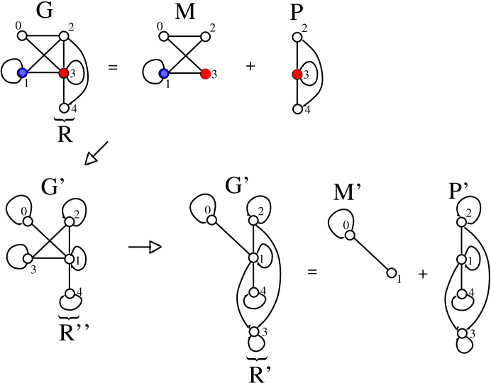
Figure 3: The action of $H_{3}$ on a two-graph state

Theorem 2

Let $\left|\psi\right>=m(-1)^{p}$ be a two-graph state over $n$ qubits. Then there always exists a graph state, $\left|\psi\right>^{\prime}$, such that $\left|\psi\right>^{\prime}=DU\left|\psi\right>$, where $U\in\{I,H\}^{\otimes n}$, and $D\in{\bf{D_{n}}}$.

Proof: Select an arbitrary $v\in{\cal{L}}$, and apply $H_{v}$ to $\left|\psi\right>$. Then, by applying the algorithm of theorem 1, we obtain $\left|\psi\right>^{(1)}=H_{v}\left|\psi\right>$, where ${\cal{L}}^{(1)}={\cal{L}}\setminus\{v\}$. Select an arbitrary $v^{\prime}\in{\cal{L}}^{(1)}$ and repeat the above process by applying $H_{v^{\prime}}$ to $\left|\psi\right>^{(1)}$ so as to obtain $\left|\psi\right>^{(2)}$, and so on. After $k=|{\cal{L}}|$ such recursions one obtains ${\cal{L}}^{(k)}=\emptyset$, which implies that $\left|\psi\right>^{(k)}$ is a graph state to within loops in $P$, as $m=1$. The loops in $P$ can then be eliminated via the action of matrices from ${\bf{D_{n}}}$.  

Corollary 1

(of theorem 2) The two-graph state is a stabilizer state.

Proof: It is known that a stabilizer state is locally-equivalent to a graph state [32, 14], and local-equivalence is reversible.  

4 The Generalised Two-Graph State

For a set of integers, ${\cal{Q}}$, let ${\cal{Q}}_{j}=1$ iff $j\in{\cal{Q}}$, otherwise ${\cal{Q}}_{j}=0$.

Definition 11

A generalised two-graph state is a pure quantum state, $\left|\psi\right>$, of $n$ qubits that can be defined by the graph-set-set, $(G,{\cal{R}},{\cal{Q}})$, where $G=({\cal{V}},{\cal{E}})$ is an $n$-vertex graph, with bipartition, $({\cal{L}},{\cal{R}})$, where ${\cal{V}}={\cal{L}}\cup{\cal{R}}$ and ${\cal{L}}\cap{\cal{R}}=\emptyset$, where $G_{\cal{L}}$ is the empty graph apart from possible loops, and where ${\cal{Q}}\subset{\cal{R}}$. The triple, $(G,{\cal{R}},{\cal Q})$, explicitly encodes a generalised two-graph, $(M,P,{\cal Q})$, where $P=G_{\cal{R},{\cal Q}}$, and $M=G-P$ is bipartite. The state, $\left|\psi\right>$, is defined by its algebraic polar form, $\left|\psi\right>=cm({\bf{x}})i^{p({\bf{x}})}$, where $c\in{\mathbb{C}}$, $m({\bf{x}}):{\mathbb{Z}}_{2}^{n}\rightarrow{\mathbb{Z}}_{2}$ is a product of affine functions of the form,

$$m({\bf{x}})=\prod_{i\in{\cal{L}}}(\Gamma_{M_{ii}}+1+x_{i}+\sum_{j\in{\cal{R}}}\Gamma_{M_{ij}}x_{j}),$$

such that $m=1$ when ${\cal{L}}=\emptyset$, and where $p({\bf{x}}):{\mathbb{Z}}_{2}^{n}\rightarrow{\mathbb{Z}}_{4}$ is a quadratic function of the form,

$$p({\bf{x}})=\sum_{i,j\in{\cal{R}},i<j}2\Gamma_{P_{ij}}x_{i}x_{j}+\sum_{j\in{\cal{R}}}(2\Gamma_{P_{jj}}+{\cal{Q}}_{j})x_{j}.$$

Remark: The generalised two-graph state can alternatively and, perhaps, more naturally, be viewed as a graph with weighted ${\mathbb{Z}}_{4}$ loops and a set ${\cal{R}}$. But we choose the equivalent $(G,{\cal{R}},{\cal{Q}})$ representation for notational convenience. When ${\cal{Q}}=\emptyset$, then the generalised two-graph state, defined by $(G,{\cal{R}},{\cal{Q}})$, reduces to the two-graph state, defined by $(G,{\cal{R}})$, and non-empty ${\cal{Q}}$ introduces linear terms over ${\mathbb{Z}}_{4}$ to the state.

Let $A\ominus B$ be the symmetric difference of sets $A$ and $B$, that is $A\ominus B=(A\setminus B)\cup(B\setminus A)$.

Definition 12

Let $(G,{\cal{Q}})$ be the graph-set pair, extracted from the generalised two-graph state $(G,{\cal{R}},{\cal{Q}})$, with $G$ an $n$-vertex graph with possible loops and ${\cal{Q}}\subset\{0,1,\ldots,n-1\}$. Then $(G,{\cal{Q}})^{v}=(G^{v},{\cal{Q}}^{v})$ is defined to be the graph-set pair resulting from the action of local complementation^⊙ (LC^⊙) on vertex $v$ of $(G,{\cal{Q}})$, where

$$\begin{array}[]{l}G^{v}=G+C_{{\cal{N}}_{v}^{G}}+\Gamma_{G_{vv}}\Delta_{{\cal{N}}_{v}^{G}}+\Delta_{{\cal{Q}}\cap{\cal{N}}_{v}^{G}},\\ {\cal{Q}}^{v}={\cal{Q}}\ominus{{\cal{B}}_{v}^{G}}.\end{array}$$

Example: The action of LC^⊙ on the following graph-set, $(G,{\cal{Q}})$, at vertex $v=3$, is shown in figure 4.

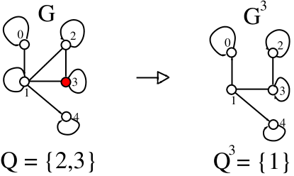
Figure 4: The action of LC^⊙ at vertex $3$

Remark: From definition 12, even when $G$ is a simple graph and ${\cal{Q}}=\emptyset$, we see that possible loops can still be produced at the output. The LC operation, which acts only on simple graphs, can be recovered from LC^⊙ by applying LC^⊙ to a simple graph, then deleting any resultant loops from the output.

We now describe the action of ‘swp’ on the generalised two-graph state at edge $vw$, as a natural extension of ‘swp’ on a two-graph state.

Definition 13

Let $\left|\psi\right>=mi^{p}$ be a generalised two-graph state over $n$ qubits, represented by the graph-set-set $(G,{\cal{R}},{\cal{Q}})\equiv(M,P,{\cal{Q}})$. Let $v\in{\cal{L}}$ and $w\in{\cal{N}}_{v}^{G}$. Then the action of swp at edge $vw$ is the operation that interchanges the roles of $v$ and $w$; i.e. the operation that takes ${\cal R}$ to ${\cal{R}}^{\prime}={\cal{R}}\cup\{v\}\setminus\{w\}$, and results in a generalised two-graph state, $m^{\prime}i^{p^{\prime}}$, where $\left|\psi\right>=m^{\prime}i^{p^{\prime}}=mi^{p}$.

Remark: ‘swp’ does not change $\left|\psi\right>$.

Lemma 2

Let $\left|\psi\right>$ be a generalised two-graph state over $n$ qubits, represented by the graph-set-set $(G,{\cal{R}},{\cal{Q}})\equiv(M,P,{\cal{Q}})$. Let $v\in{\cal{L}}$ and $w\in{\cal{N}}_{v}^{G}$. Then the action of swp at edge $vw$ results in the generalised two-graph state with associated graph-set-set, $(G^{\prime},{\cal{R}}^{\prime},{\cal{Q}}^{\prime})\equiv(M^{\prime},P^{\prime},{\cal{Q}}^{\prime})$, and is obtained from $(G,{\cal{R}},{\cal{Q}})$ as follows:

Let $v\in{\cal{L}},w\in{\cal{N}}_{v}^{G}$. Then, $(G^{\prime},{\cal{R}}^{\prime},{\cal{Q}}^{\prime})=\mbox{\bf{swp}}(G,{\cal{R}},{\cal{Q}},v,w)$ can be expressed as:

$$\begin{array}[]{l}\left\{\begin{array}[]{l}{\cal{R}}^{\prime}={\cal{R}}\cup\{v\}\setminus\{w\},\\ G^{\prime\prime}=G^{vw},\\ \mbox{if }{\cal{Q}}_{w}=1\\ \hskip 14.22636pt\mbox{ }(G^{\prime},{\cal{Q}}^{\prime})=(G^{\prime\prime},{\cal{Q}})^{w}\\ \mbox{else }\\ \hskip 14.22636pt\mbox{ }(G^{\prime},{\cal{Q}}^{\prime})=(G^{\prime\prime},{\cal{Q}}).\end{array}\right.\end{array}$$

Proof: Section 7.  

We now describe the action of $H_{v}$ on a generalised two-graph state.

Theorem 3

Let $\left|\psi\right>$ be a generalised two-graph state over $n$ qubits, represented by the graph-set-set $(G,{\cal{R}},{\cal{Q}})\equiv(M,P,{\cal{Q}})$. Let $v\in\{0,1,\ldots,n-1\}$. Then $\left|\psi^{\prime}\right>=H_{v}\left|\psi\right>$ is also a generalised two-graph state and can be described by the graph-set-set $(G^{\prime},{\cal{R}}^{\prime},{\cal{Q}}^{\prime})\equiv(M^{\prime},P^{\prime},{\cal{Q}}^{\prime})$, where

$(G^{\prime},{\cal{R}}^{\prime},{\cal{Q}}^{\prime})=H_{v}(G,{\cal{R}},{\cal{Q}})$:

$$\begin{array}[]{ll}\left\{\begin{array}[]{l}{\cal{R}}^{\prime}={\cal{R}}\cup\{v\},\\ (G^{\prime},{\cal{Q}}^{\prime})=(G,{\cal{Q}}),\end{array}\right.&\hskip 14.22636pt\mbox{ }\mbox{ if }v\in{\cal{L}},\\ \\ \left\{\begin{array}[]{l}\mbox{if }{\cal{Q}}_{v}=0\\ \hskip 14.22636pt\mbox{ }{\cal{R}}^{\prime}={\cal{R}}\setminus\{v\},\\ \hskip 14.22636pt\mbox{ }(G^{\prime},{\cal{Q}}^{\prime})=(G,{\cal{Q}}),\\ \mbox{else }\\ \hskip 14.22636pt\mbox{ }{\cal{R}}^{\prime}={\cal{R}},\\ \hskip 14.22636pt\mbox{ }(G^{\prime\prime},{\cal{Q}}^{\prime\prime})=(G,{\cal{Q}})^{v}\\ \hskip 14.22636pt\mbox{ }G^{\prime}=G^{\prime\prime}+\Delta_{{\cal{B}}_{v}^{G}}\\ \hskip 14.22636pt\mbox{ }{\cal Q}^{\prime}={\cal Q}^{\prime\prime}\cup\{v\}\enspace,\end{array}\right.&\hskip 14.22636pt\mbox{ }\mbox{ if }{\cal{B}}_{v}^{G}\subseteq{\cal{R}}\\ \\ \left\{\begin{array}[]{l}\mbox{assign }w\in{\cal{N}}_{v}^{M},\\ (G^{\prime},{\cal{R}}^{\prime\prime},{\cal{Q}}^{\prime})=\mbox{swp}(G,{\cal{R}},{\cal{Q}},w,v),\\ {\cal{R}}^{\prime}={\cal{R}}^{\prime\prime}\cup\{v\},\end{array}\right.&\hskip 14.22636pt\mbox{ }\mbox{ if }v\in{\cal{R}},{\cal{B}}_{v}^{G}\not\nsubseteq{\cal{R}}.\end{array}$$

Proof: Section 7.  

Example: Let $\left|\psi\right>=mi^{p}$ be a generalised two-graph state, with $n=5$, $m=(x_{0}+x_{2}+x_{3}+1)(x_{1}+x_{2}+x_{3})$, $p=2x_{2}x_{3}+2x_{2}x_{4}+2x_{3}x_{4}+x_{2}+3x_{3}$, and graph $(G,{\cal{R}},{\cal{Q}})\equiv(M,P,{\cal{Q}})$, where $G$ has edge set ${\cal{E}}=\{02,03,12,13,23,24,34,11,33\}$, ${\cal{R}}=\{2,3,4\}$, and ${\cal{Q}}=\{2,3\}$. Then the action of $H_{3}$ on $\left|\psi\right>$ can be detailed as follows where we, arbitrarily, choose $w=1$. Then ${\cal{R}}^{\prime}=\{1,2,3,4\}$ and ${\cal{Q}}^{\prime}=\{1,2,3,4\}$. The resulting graph, $(G^{\prime},{\cal{R}}^{\prime},{\cal{Q}}^{\prime})\equiv(M^{\prime},P^{\prime},Q^{\prime})$, represents the generalised two-graph state $\left|\psi^{\prime}\right>=m^{\prime}i^{p^{\prime}}$, where $m^{\prime}=(x_{0}+x_{1})$ and $p^{\prime}=2x_{1}x_{3}+2x_{1}x_{4}+2x_{2}x_{3}+x_{2}+x_{3}+x_{4}$. This example is illustrated in figure 5.

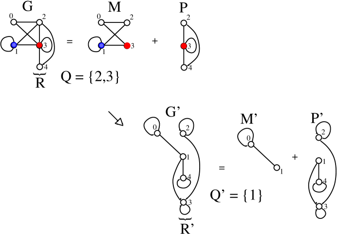
Figure 5: The action of $H_{3}$ on a generalised two-graph state

We now describe the action of $N_{v}$ on a generalised two-graph state.

Theorem 4

Let $\left|\psi\right>$ be a generalised two-graph state over $n$ qubits, represented by the graph-set-set $(G,{\cal{R}},{\cal{Q}})\equiv(M,P,{\cal{Q}})$. Let $v\in\{0,1,\ldots,n-1\}$. Then $\left|\psi^{\prime}\right>=N_{v}\left|\psi\right>$ is also a generalised two-graph state and can be described by the graph-set-set $(G^{\prime},{\cal{R}}^{\prime},{\cal{Q}}^{\prime})\equiv(M^{\prime},P^{\prime},{\cal{Q}}^{\prime})$, where

$(G^{\prime},{\cal{R}}^{\prime},{\cal{Q}}^{\prime})=N_{v}(G,{\cal{R}},{\cal{Q}})$:

$$\begin{array}[]{ll}\left\{\begin{array}[]{l}{\cal{R}}^{\prime}={\cal{R}}\cup\{v\},\\ (G^{\prime},{\cal{Q}}^{\prime\prime})=(G,{\cal{Q}})^{v},\\ {\cal{Q}}^{\prime}={\cal{Q}}^{\prime\prime}\setminus\{v\},\end{array}\right.&\hskip 14.22636pt\mbox{ }\mbox{ if }v\in{\cal{L}},\\ \\ \left\{\begin{array}[]{l}\mbox{if }{\cal{Q}}_{v}=1\\ \hskip 14.22636pt\mbox{ }{\cal{R}}^{\prime}={\cal{R}}\setminus\{v\},\\ \hskip 14.22636pt\mbox{ }G^{\prime}=G+\Delta_{\{v\}},\\ \hskip 14.22636pt\mbox{ }{\cal{Q}}^{\prime}={\cal{Q}}\setminus\{v\},\\ \mbox{else }\\ \hskip 14.22636pt\mbox{ }{\cal{R}}^{\prime}={\cal{R}},\\ \hskip 14.22636pt\mbox{ }(G^{\prime\prime},{\cal{Q^{\prime}}})=(G,{\cal{Q}})^{v}\\ \hskip 14.22636pt\mbox{ }G^{\prime}=G^{\prime\prime}+\Delta_{{\cal{B}}_{v}^{G}}\enspace,\end{array}\right.&\hskip 14.22636pt\mbox{ }\mbox{ if }{\cal{B}}_{v}^{G}\subseteq{\cal{R}}\\ \\ \left\{\begin{array}[]{l}\mbox{assign }w\in{\cal{N}}_{v}^{M},\\ (G^{\prime\prime},{\cal{R}}^{\prime\prime},{\cal{Q}}^{\prime\prime})=\mbox{swp}(G,{\cal{R}},{\cal{Q}},w,v),\\ {\cal{R}}^{\prime}={\cal{R}}^{\prime\prime}\cup\{v\},\\ (G^{\prime},{\cal{Q}}^{\prime\prime\prime})=(G^{\prime\prime},{\cal{Q}}^{\prime\prime})^{v},\\ {\cal{Q}}^{\prime}={\cal{Q}}^{\prime\prime\prime}\setminus\{v\},\end{array}\right.&\hskip 14.22636pt\mbox{ }\mbox{ if }v\in{\cal{R}},{\cal{B}}_{v}^{G}\not\nsubseteq{\cal{R}}.\end{array}$$

Proof: Section 7.  

We now describe the action of the inverse of $N_{v}$ on a generalised two-graph state. This is important for computational reasons, as it allows us to compute spectral measures such as the $L_{j}$ norm and the Clifford merit factor [24] of a graph state (section 6) by using a Gray code ordering on successive actions of $H$ and $N$ on each qubit, thereby avoiding the problem of having to store all the graphs from every step.

Lemma 3

Let $\left|\psi\right>$ be a generalised two-graph state over $n$ qubits, represented by the graph-set-set $(G,{\cal{R}},{\cal{Q}})\equiv(M,P,{\cal{Q}})$. Let $(G^{\prime\prime},{\cal{R}}^{\prime\prime},{\cal{Q}}^{\prime\prime})\equiv(M^{\prime\prime},P^{\prime\prime},{\cal{Q}}^{\prime\prime})$ be the generalised two-graph state resulting from the application of $H_{v}$ to $(G,{\cal{R}},{\cal{Q}})$. Let $v\in\{0,1,\ldots,n-1\}$. Then the action of $N^{-1}$ on $v$ is the graph-set-set $(G^{\prime},{\cal{R}}^{\prime},{\cal{Q}}^{\prime})\equiv(M^{\prime},P^{\prime},{\cal{Q}}^{\prime})$, where:

$$\begin{array}[]{ll}\left\{\begin{array}[]{l}G^{\prime}=G^{\prime\prime}+C_{{\cal N}_{v}^{G^{\prime\prime}}}+\Delta_{{\cal N}_{v}^{G^{\prime\prime}}}+\Gamma_{vv}^{G^{\prime\prime}}\Delta_{{\cal N}_{v}^{G^{\prime\prime}}}+\Delta_{{\cal Q}^{\prime\prime}\cap{\cal N}_{v}^{G^{\prime\prime}}}\\ {\cal Q}^{\prime}={\cal Q}^{\prime\prime}\ominus{\cal N}_{v}^{G^{\prime\prime}}\end{array}\right.&\mbox{ if }v\in{\cal L}^{\prime\prime}\\ \\ \left\{\begin{array}[]{l}G^{\prime}=G^{\prime\prime}+\Delta_{v}\\ {\cal Q}^{\prime}={\cal Q}^{\prime\prime}\cup\{v\}\end{array}\right.&\mbox{ if }v\in{\cal R}^{\prime\prime}\mbox{ and }{\cal Q}_{v}^{\prime\prime}=0\\ \\ \left\{\begin{array}[]{l}G^{\prime}=G^{\prime\prime}\\ {\cal Q}^{\prime}={\cal Q}^{\prime\prime}\setminus\{v\}\end{array}\right.&\mbox{ if }v\in{\cal R}^{\prime\prime}\mbox{ and }{\cal Q}_{v}^{\prime\prime}=1\\ {\cal{R}}^{\prime}={\cal{R}}^{\prime\prime}.&\end{array}$$

Proof: Section 7.  

Theorem 5

Let $\left|\psi\right>=mi^{p}$ be a generalised two-graph state over $n$ qubits. Then there always exists a graph state, $\left|\psi\right>^{\prime}$, such that $\left|\psi\right>^{\prime}=U\left|\psi\right>$, where $U\in{\bf{C_{n}}}$.

Proof: A generalised two-graph state, $(G,{\cal{R}},{\cal{Q}})$ is always locally-equivalent to a two-graph state, $(G,{\cal{R}})=(G,{\cal{R}},{\cal{Q}}^{\prime})$, via the action of some unitary in ${\bf{D_{n}}}$, where ${\cal{Q}}^{\prime}=\emptyset$. The theorem then follows from theorem 2.  

Corollary 2

(theorem 5) The generalised two-graph state is a stabilizer state, and vice-versa.

Proof: From [14, 32] and theorem 5, all stabilizer states and all generalised two-graph states are graph states, via the action of unitaries from the local Clifford group, and such action is reversible.  

4.1 The actions of $\lambda$ and $\lambda^{2}$

We have described the action of $N$ and $H$ on the generalised two-graph state. It is trivial to convert these actions to the actions of $\lambda$ and $\lambda^{2}$ on the state, respectively, remembering that, in this paper, global multiplicative constants are ignored. Explicitly,

$$\lambda_{v}(G,{\cal{R}},{\cal{Q}})=N_{v}(G,{\cal{R}},{\cal{Q}}),\hskip 14.22636pt\mbox{ }\hskip 14.22636pt\mbox{ }\lambda_{v}^{2}(G,{\cal{R}},{\cal{Q}})=S_{v}^{-1}H_{v}(G,{\cal{R}},{\cal{Q}})=N_{v}^{2}(G,{\cal{R}},{\cal{Q}}).$$

5 Canonisation

For some (generalised) two-graph state, $mi^{p}$, as represented by $(G,{\cal{R}},{\cal{Q}})$ over $n$ qubits, let ${\cal{L}}\neq\emptyset$. Then there is a set of equivalent representations for the same state. For purposes of comparison, it is desirable to find a canonical representative from each set of equivalent representations. In this section we provide a simple algorithm to obtain, from an arbitrary (generalised) two-graph state, a canonical representative.

Definition 14

A generalised two-graph state, $(G,{\cal{R}},{\cal{Q}})$, is defined to be canonised if $v<u$, $\forall(v,u)\in({\cal{L}},{\cal{N}}_{v}^{G})$.

Observe that such a canonical form is unique and, given such a unique $M$ graph, the $P$ graph and $Q$ set are also unambiguously fixed. We now describe the process of canonisation of a generalised two-graph state.

Lemma 4

Let $\left|\psi\right>$ be a generalised two-graph state over $n$ qubits, as represented by $(G,{\cal{R}},{\cal{Q}})$. Then we can obtain a canonical representation of $\left|\psi\right>$, as represented by $(G_{n},{\cal{R}}_{n},{\cal{Q}}_{n})$, by following these steps, where $\min({\cal{A}})$ means the minimum integer in set ${\cal{A}}$:

$(G_{n},{\cal{R}}_{n},{\cal{Q}}_{n})=$ canon$(G,{\cal{R}},{\cal{Q}})$:

$$\begin{array}[]{l}\left\{\begin{array}[]{l}\mbox{Set }(G_{0},{\cal{R}}_{0},{\cal{Q}}_{0})=(G,{\cal{R}},{\cal{Q}}),\mbox{ and set }i=0\\ \mbox{while }\exists v\in{\cal L}_{i}\mbox{ such that }v>\min({\cal N}_{v}^{G_{i}})\\ \hskip 14.22636pt\mbox{ }\hskip 14.22636pt\mbox{ }w=\min({\cal N}_{v}^{G_{i}})\\ \hskip 14.22636pt\mbox{ }\hskip 14.22636pt\mbox{ }(G_{i+1},{\cal{R}}_{i+1},{\cal{Q}}_{i+1})=\mbox{swp}(G_{i},{\cal{R}}_{i},{\cal{Q}}_{i},v,w)\\ \hskip 14.22636pt\mbox{ }\hskip 14.22636pt\mbox{ }i\leftarrow i+1.\end{array}\right.\end{array}$$

Each call to canon will have worst-case complexity $O(|{\cal L}|^{2})$.

Proof: Section 7.  

One can apply canonisation to the generalised two-graph state after each application of $N$ or $H$, if required.

6 Spectral Analysis of the Graph State

We now briefly demonstrate the usefulness of the two-graph representation by computing various $L_{j}$-norms of the graph state wrt the local Clifford group. Let $\left|\psi\right>$ be a generalised two-graph state over $n$ qubits. For $U\in{\bf{C_{n}}}$, let $\left|\psi_{U}\right>=U\left|\psi\right>$. The $L_{j}$-norm of $\left|\psi\right>$ is given by

$$||\left|\psi\right>||_{j}=\left(2^{-n}\sum_{{\bf{x}}\in{\mathbb{Z}}_{2}^{n}}(2^{\frac{n}{2}}|\left|\psi\right>_{\bf{x}}|)^{j}\right)^{\frac{1}{j}}=2^{n(\frac{1}{2}-\frac{1}{j})}\left(\sum_{{\bf{x}}\in{\mathbb{Z}}_{2}^{n}}|\left|\psi\right>_{\bf{x}}|^{j}\right)^{\frac{1}{j}}.$$

We wish to compute the $L_{j}$-norm over every state generated by the action of the local Clifford group on $\left|\psi\right>$. However, as these norms only depend on a summary of powers of magnitudes, it suffices to compute the $L_{j}$-norm over every state generated by the action of $\{I,H,N\}^{\otimes n}$ on $\left|\psi\right>$, as the action of matrices from ${\bf D_{n}}$ on the state does not affect coefficient magnitudes; that is, let $U=U_{D}U_{T}$, with $U_{D}\in{\bf D_{n}}$ and $U_{T}\in\{I,H,N\}^{\otimes n}$: then $||\left|\psi_{U}\right>||=||\left|\psi_{U_{D}U_{T}}\right>||=||\left|\psi_{U_{T}}\right>||$. Thus

$$||\left|\psi\right>||_{{\bf{C_{n}}},j}=\left(\frac{24^{-n}}{8}\sum_{U\in{\bf{C_{n}}}}||\left|\psi_{U}\right>||_{j}^{j}\right)^{\frac{1}{j}}=\left(3^{-n}\sum_{U\in\{I,H,N\}^{\otimes n}}||\left|\psi_{U}\right>||_{j}^{j}\right)^{\frac{1}{j}}=2^{\frac{n}{2}}\left(6^{-n}\sum_{\tiny\begin{array}[]{c}{\bf{x}}\in{\mathbb{Z}}_{2}^{n}\\ U\in\{I,H,N\}^{\otimes n}\end{array}}|\left|\psi_{U}\right>_{\bf{x}}|^{j}\right)^{\frac{1}{j}}.$$

Normalisation of the pure state ensures that $||\left|\psi\right>||_{2}=||\left|\psi\right>||_{{\bf{C_{n}}},2}=1$, by Parseval’s theorem.

Let $\left|\psi_{U}\right>$ be represented by the graph-set-set $(G_{U},{\cal{R}}_{U},{\cal{Q}}_{U})$, where ${\cal{L}}_{U}={\cal{V}}\setminus{\cal{R}}_{U}$. Then one can show that,

$$||\left|\psi_{U}\right>||_{j}=2^{\frac{(j-2)|{\cal{L}}_{U}|}{2j}}.$$

Therefore,

$$||\left|\psi\right>||_{{\bf{C_{n}}},j}=\left(3^{-n}\sum_{U\in\{I,H,N\}^{\otimes n}}2^{\frac{(j-2)|{\cal{L}}_{U}|}{2}}\right)^{\frac{1}{j}}.$$

In other words, $||\left|\psi\right>||_{{\bf{C_{n}}},j}$ can be efficiently computed by keeping track of the size of ${\cal{L}}_{U}$ after each successive action of $H$ and $N$ on the two-graph state. In particular, although the evaluation is theoretically over all $24^{n}\times 8$ transforms represented by the local Clifford group, we obtain the same evaluation by only considering the $3^{n}$ transforms represented by $\{I,H,N\}^{\otimes n}$, which is an exponential improvement in computational complexity.

Using the Database of Self-Dual Quantum Codes [5] we classify all inequivalent graph states according to their $L_{j}$ norms wrt ${\bf{C_{n}}}$, up to $n=7$ qubits, as shown in table 1 for $j=3$ and $j=4$, where the norm is $||\left|\psi\right>||_{{\bf{C_{n}}},j}$. One can expect the entanglement of the graph state to be higher if $||\left|\psi\right>||_{{\bf{C_{n}}},j}$ is lower. In [24], the so-called Clifford merit factor (${\cal{CMF}}$) was proposed as a suitable measure of entanglement for a graph state, where

$${\cal{CMF}}(\left|\psi\right>)=\frac{1}{||\left|\psi\right>||_{{\bf{C_{n}}},4}^{4}-1}.$$

One can expect the entanglement of a graph state to be higher if the CMF of a graph state is higher. Moreover, it was proved in [24] that the expected value of $\frac{1}{\cal{CMF}}$ for a random graph state, as $n\rightarrow\infty$, is $1$ . This is suggested as, at least, reasonable by the results of table 1 as $||\left|\psi\right>||_{{\bf{C_{n}}},4}^{4}$ for a random graph state could well approach $2$ from below as $n\rightarrow\infty$.

$\begin{array}[]{cc}\begin{array}[]{|c|c|c|}\hline\cr n&||\left|\psi\right>||_{{\bf{C_{n}}},3}&\mbox{frequency}\\ \hline\cr\hline\cr 1&1.000000&1\\ \hline\cr\mbox{average}&1.000000&1\\ \hline\cr\hline\cr 2&1.000000&1\\ \hline\cr\mbox{average}&1.000000&1\\ \hline\cr\hline\cr 3&1.079871&1\\ \hline\cr\mbox{average}&1.079871&1\\ \hline\cr\hline\cr 4&1.035744&1\\ \cline{2-3}\cr&1.020167&1\\ \hline\cr\mbox{average}&1.027955&2\\ \hline\cr\hline\cr 5&1.067977&1\\ \cline{2-3}\cr&1.040834&1\\ \cline{2-3}\cr&1.030604&1\\ \cline{2-3}\cr&1.020167&1\\ \hline\cr\mbox{average}&1.039895&4\\ \hline\cr\hline\cr 6&1.106649&1\\ \cline{2-3}\cr&1.071174&1\\ \cline{2-3}\cr&1.059898&1\\ \cline{2-3}\cr&1.053345&1\\ \cline{2-3}\cr&1.047544&1\\ \cline{2-3}\cr&1.046710&1\\ \cline{2-3}\cr&1.040834&2\\ \cline{2-3}\cr&1.034036&1\\ \cline{2-3}\cr&1.027148&1\\ \cline{2-3}\cr&1.020167&1\\ \hline\cr\mbox{average}&1.049849&11\\ \hline\cr\hline\cr 7&1.150213&1\\ \cline{2-3}\cr&1.108636&1\\ \cline{2-3}\cr&1.089457&1\\ \cline{2-3}\cr&1.085332&1\\ \cline{2-3}\cr&1.078038&1\\ \cline{2-3}\cr&1.075408&1\\ \cline{2-3}\cr&1.073824&1\\ \cline{2-3}\cr&1.067977&1\\ \cline{2-3}\cr&1.063683&2\\ \cline{2-3}\cr&1.059898&1\\ \cline{2-3}\cr&1.059355&1\\ \cline{2-3}\cr&1.056085&1\\ \cline{2-3}\cr&1.055538&1\\ \cline{2-3}\cr&1.051694&2\\ \cline{2-3}\cr&1.051143&1\\ \cline{2-3}\cr&1.047266&1\\ \cline{2-3}\cr&1.043080&1\\ \cline{2-3}\cr&1.042800&1\\ \cline{2-3}\cr&1.038578&1\\ \cline{2-3}\cr&1.034036&3\\ \cline{2-3}\cr&1.033751&1\\ \cline{2-3}\cr&1.029455&1\\ \hline\cr\mbox{average}&1.060719&26\\ \hline\cr\hline\cr\end{array}&\begin{array}[]{|c|c|c|c|}\hline\cr n&||\left|\psi\right>||_{{\bf{C_{n}}},4}&\mbox{CMF}&\mbox{frequency}\\ \hline\cr\hline\cr 1&1.074570&3.000000&1\\ \hline\cr\mbox{average}1&1.074570&&1\\ \hline\cr\hline\cr 2&1.074570&3.000000&1\\ \hline\cr\mbox{average}&1.074570&&1\\ \hline\cr\hline\cr 3&1.240806&0.729730&1\\ \hline\cr\mbox{average}&1.240806&&1\\ \hline\cr\hline\cr 4&1.154701&1.285714&1\\ \cline{2-4}\cr&1.121195&1.723404&1\\ \hline\cr\mbox{average}&1.137948&&2\\ \hline\cr\hline\cr 5&1.223202&0.807309&1\\ \cline{2-4}\cr&1.165247&1.185366&1\\ \cline{2-4}\cr&1.143857&1.404624&1\\ \cline{2-4}\cr&1.121195&1.723404&1\\ \hline\cr\mbox{average}&1.163375&&4\\ \hline\cr\hline\cr 6&1.304643&0.527115&1\\ \cline{2-4}\cr&1.229154&0.779679&1\\ \cline{2-4}\cr&1.204803&0.903346&1\\ \cline{2-4}\cr&1.192052&0.981157&1\\ \cline{2-4}\cr&1.178878&1.073638&2\\ \cline{2-4}\cr&1.165247&1.185366&2\\ \cline{2-4}\cr&1.151120&1.323049&1\\ \cline{2-4}\cr&1.136453&1.496920&1\\ \cline{2-4}\cr&1.121195&1.723404&1\\ \hline\cr\mbox{average}&1.184334&&11\\ \hline\cr\hline\cr 7&1.396589&0.356595&1\\ \cline{2-4}\cr&1.307925&0.519108&1\\ \cline{2-4}\cr&1.266787&0.634833&1\\ \cline{2-4}\cr&1.259527&0.659331&1\\ \cline{2-4}\cr&1.244619&0.714472&1\\ \cline{2-4}\cr&1.236959&0.745653&2\\ \cline{2-4}\cr&1.221198&0.816959&1\\ \cline{2-4}\cr&1.213084&0.857984&2\\ \cline{2-4}\cr&1.204803&0.903346&2\\ \cline{2-4}\cr&1.196347&0.953772&2\\ \cline{2-4}\cr&1.187709&1.010162&3\\ \cline{2-4}\cr&1.178878&1.073638&1\\ \cline{2-4}\cr&1.169844&1.145626&2\\ \cline{2-4}\cr&1.160595&1.227962&1\\ \cline{2-4}\cr&1.151120&1.323049&4\\ \cline{2-4}\cr&1.141405&1.434098&1\\ \hline\cr\mbox{average}&1.207200&&26\\ \hline\cr\hline\cr\end{array}\end{array}$

Table 1: $||\left|\psi\right>||_{{\bf{C_{n}}},3}$ and $||\left|\psi\right>||_{{\bf{C_{n}}},4}$ norms for graph states of $n=1$ to $7$ vertices

We can also compute the $L_{\infty}$ norm of a graph state wrt the local Clifford group, where,

$$||\left|\psi\right>||_{{\bf{C_{n}}},\infty}=2^{\left(\sup_{U\in\{I,H,N\}^{\otimes n}}(|{\cal{L}}_{U}|)\right)/2},$$

and (potentially) ranges from $1$ to $2^{n/2}$ (although, for connected graphs, neither the ‘ideal’ lower bound or the worst-case upper-bound are ever reached). In [4] the PAR_IHN, of a graph state is computed, where PAR${}_{IHN}(\left|\psi\right>)=||\left|\psi\right>||_{{\bf{C_{n}}},\infty}^{2}$, and where $n-\log_{2}(\mbox{PAR}_{IHN})$ gives a lower bound on the entanglement of the graph state as measured by the log form of the geometric measure [38], which is an entanglement monotone [37]. This lower bound is shown to be tight for a graph state with a bipartite graph in its LC orbit [22, 4]. The method used in [4] to compute PAR_IHN looked for the independent set of largest size over the set of graphs in the LC orbit of $\left|\psi\right>$. It is evident that $\sup_{U\in\{I,H,N\}^{\otimes n}}(|{\cal{L}}_{U}|)$ is equal to the size of this largest independent set. So we do not strictly need the two-graph form to compute the $L_{\infty}$-norm of the graph state, but can make do with LC over the graph state. However, we then require to search for the largest independent set in each graph in the LC orbit. In contrast, if we use the two-graph representation to compute the $L_{\infty}$-norm of the graph state then we identify an independent set in the current graph wrt $U$ as being the set ${\cal{L}}_{U}$. Thus the two-graph representation implicitly encodes and keeps track of the independent sets in the graphs in the LC orbit of the graph state. The search techniques of [4] and this paper are of approximately equal computational complexity. Results for PAR_IHN for graph states are provided in [4]. In figure 6 we plot the expected PAR_IHN of a graph state of varying density, where the ‘density’ indicates the percentage probability that a given edge exists. From figure 6 we conclude that very dense and very sparse graphs represent graph states with relatively high values of PAR_IHN, which translates to a relatively low lower bound on the geometric measure of entanglement. Therefore, as one might expect, it appears that graph states of density around $0.5$ should maximise the lower bound on the geometric measure of entanglement.

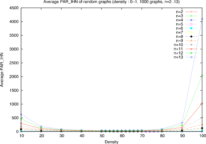
Figure 6: Expected PAR_IHN of random graph states of $n=2$ to $13$ vertices versus graph density, $10-100$%

In figure 7 we compute the expected value for an $L_{j}$ norm, $2\leq j<16$, for a random graph state of density 50%. The horizontal lines are the results for the $L_{\infty}$ norm, where $||\left|\psi\right>||_{{\bf{C_{n}}},\infty}=\sqrt{\mbox{PAR}_{IHN}}$. The results indicate that the $L_{\infty}$ norm is approached from below by the $L_{j}$ norm as $j\rightarrow\infty$ (it is not so difficult to prove this). The results also indicate that the relationship between expected $||\left|\psi\right>||_{{\bf{C_{n}}},\infty}$ and $n$ is marginally superlinear, at least for small numbers of vertices.

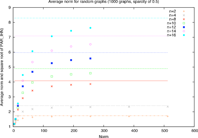
Figure 7: Expected $L_{j}$ norm and $\sqrt{\mbox{PAR}_{IHN}}$ versus $j$ for $n$-vertex random graph states

7 Appendix: Proofs

For an integer set, ${\cal S}$, denote $x_{\cal S}=\sum_{j\in{\cal S}}x_{j}$, and let $x_{a}\in f$, $x_{a}\not\in f$, mean that $f$ is or is not dependent on $x_{a}$, respectively. We denote $p_{a}=p_{x_{v}=a}$, $m_{a}=m|_{x_{v}=a}$, for $a\in{\mathbb{Z}}_{2}$.

7.1 Proofs for section 3

Proof: (of lemma 1) We write $m=r(x_{v}+x_{w}+h_{v})\ \prod_{t\in{\cal N}_{w}^{M}\setminus\{v\}}(x_{t}+x_{w}+h_{t})$, with $x_{v},x_{w}\notin r$, for $h_{k}=\Gamma_{M_{kk}}+1+\sum_{j\in{\cal N}_{k}^{M}\setminus\{w\}}x_{j}$. We also write $p=x_{w}(x_{{\cal N}_{w}^{P}}+\Gamma_{P_{ww}})+p|_{x_{w}=0}$. We want to interchange the roles of $v$ and $w$ by re-factoring $m$ and by substituting $x_{w}=x_{v}+h_{v}+1$ in the remaining terms that involve $x_{w}$. Thus $m^{\prime}=r(x_{w}+x_{v}+h_{v})\prod_{t\in{\cal N}_{w}^{M}\setminus\{v\}}(x_{t}+x_{v}+h_{v}+h_{t}+1)$, and $p^{\prime}=(x_{v}+h_{v}+1)(x_{{\cal N}_{w}^{P}}+\Gamma_{P_{ww}})+p|_{x_{w}=0}$. From the form of $m$, $p$, and $m^{\prime}$, $p^{\prime}$, where ${\cal R}^{\prime}={\cal R}\cup\{v\}\setminus\{w\}$, we obtain the graph equations,

$$\begin{array}[]{l}M^{\prime}=M-K_{\{v\},{\cal N}_{v}^{M}}-K_{{\cal N}_{w}^{M}\setminus\{v\},\{w\}}-\Gamma_{M_{vv}}\Delta_{\{v\}}+K_{\{w\},{\cal B}_{v}^{M}\setminus\{w\}}+K_{{\cal N}_{w}^{M}\setminus\{v\},{\cal B}_{v}^{M}\setminus\{w\}}+\Gamma_{M_{vv}}(\Delta_{\{w\}}+\Delta_{{\cal N}_{w}^{M}\setminus\{v\}}),\\ P^{\prime}=P-K_{\{w\},{\cal N}_{w}^{P}}-\Gamma_{P_{ww}}\Delta_{\{w\}}+K_{{\cal B}_{v}^{M}\setminus\{w\},{\cal N}_{w}^{P}}+\Gamma_{M_{vv}}\Delta_{{\cal N}_{w}^{P}}+\Gamma_{P_{ww}}\Delta_{{\cal B}_{v}^{M}\setminus\{w\}}.\end{array}$$

Rearranging,

$$\begin{array}[]{l}M^{\prime}=M+K_{\{v\},{\cal N}_{v}^{M}}+K_{{\cal N}_{w}^{M}\setminus\{v\},{\cal B}_{v}^{M}}+\Gamma_{M_{vv}}\Delta_{{\cal B}_{w}^{M}\setminus\{v\}},\\ P^{\prime}=P+K_{{\cal B}_{v}^{M},{\cal N}_{w}^{P}}+K_{\{w\},{\cal B}_{v}^{M}\setminus\{w\}}+\Gamma_{M_{vv}}\Delta_{{\cal N}_{w}^{P}}+\Gamma_{P_{ww}}\Delta_{{\cal B}_{v}^{M}\setminus\{w\}}.\end{array}$$

Combining and simplifying,

$$\begin{array}[]{ll}G^{\prime}=M^{\prime}+P^{\prime}&=G+K_{{\cal N}_{w}^{M},{\cal B}_{v}^{M}}+\Delta_{\{v\}}+K_{{\cal B}_{v}^{M},{\cal B}_{w}^{P}}+\Delta_{\{w\}}+\Gamma_{G_{vv}}\Delta_{{\cal B}_{w}^{G}}+\Gamma_{G_{ww}}\Delta_{{\cal B}_{v}^{G}}\\ &=G+K_{{\cal B}_{v}^{G},{\cal B}_{w}^{G}}+\Delta_{\{v,w\}}+\Gamma_{G_{vv}}\Delta_{{\cal B}_{w}^{G}}+\Gamma_{G_{ww}}\Delta_{{\cal B}_{v}^{G}}=G^{vw}.\end{array}$$

 

To prove theorem 1 we require the following lemma.

Lemma 5

Let $m$ and $p$ be Boolean functions. Then,

$$\sqrt{2}H_{v}m(-1)^{p}=m_{0}(-1)^{p_{0}}+m_{1}(-1)^{p_{1}+x_{v}}.$$ (1)

Proof: (lemma 1) Without loss of generality we set $v=n-1$. Then we write the $2^{n}\times 1$ vector

$$m(-1)^{p}=\left(\tiny\begin{array}[]{c}m_{0}(-1)^{p_{0}}\\ m_{1}(-1)^{p_{1}}\end{array}\right).$$

Using the equality $\sqrt{2}H=X+Z$,

$$H_{n}m(-1)^{p}=\frac{1}{\sqrt{2}}\left(X_{n-1}\left(\tiny\begin{array}[]{c}m_{0}(-1)^{p_{0}}\\ m_{1}(-1)^{p_{1}}\end{array}\right)+Z_{n-1}\left(\tiny\begin{array}[]{c}m_{0}(-1)^{p_{0}}\\ m_{1}(-1)^{p_{1}}\end{array}\right)\right)=\frac{1}{\sqrt{2}}\left(\left(\tiny\begin{array}[]{c}m_{1}(-1)^{p_{1}}\\ m_{0}(-1)^{p_{0}}\end{array}\right)+\left(\tiny\begin{array}[]{c}m_{0}(-1)^{p_{0}}\\ -m_{1}(-1)^{p_{1}}\end{array}\right)\right).$$

 

Proof: (theorem 1)

For $x_{v}\notin m$ (i.e. ${\cal B}_{v}^{G}\subseteq{\cal R}$), we only need to show that $\left|\psi^{\prime}\right>=\frac{1}{\sqrt{2}}m^{\prime}(-1)^{p^{\prime}}=H_{v}m(-1)^{p}$, where

$$m^{\prime}=m(x_{{\cal B}_{v}^{P}}+1),\ \ \ p^{\prime}=p_{0}\enspace,$$ (2)

as this implies that $M^{\prime}=M+P_{v}$, $P^{\prime}=P-P_{v}$, $G^{\prime}=M^{\prime}+P^{\prime}=G$, and $v\in{\cal L}^{\prime}$, as required. By lemma 1, and given that $x_{v}\notin m$, $\sqrt{2}H_{v}m(-1)^{p}=m(-1)^{p_{0}}(1+(-1)^{x_{{\cal B}_{v}^{P}}})=\left\{\begin{array}[]{ccl}0&\mbox{ if }&x_{{\cal B}_{v}^{P}}=1\mbox{ mod }2\\ (-1)^{p_{0}}&\mbox{ if }&x_{{\cal B}_{v}^{P}}=0\mbox{ mod }2,\end{array}\right.$ thereby proving equation (2) and the case where $x_{v}\notin m$.

For $v\in{\cal L}$, then $p_{0}=p_{1}=p$, and

$$m_{0}+(-1)^{x_{v}}m_{1}=(-1)^{x_{v}(\Gamma_{M_{vv}}+x_{{\cal N}_{v}^{G}})}\frac{m}{(\Gamma_{M_{vv}}+1+x_{{\cal B}_{v}^{G}})}.$$

Then, from lemma 1,

$$m^{\prime}=\frac{m}{(\Gamma_{M_{vv}}+1+x_{{\cal B}_{v}^{G}})},\hskip 14.22636pt\mbox{ }\mbox{ and }\hskip 14.22636pt\mbox{ }p^{\prime}=p+x_{v}(\Gamma_{M_{vv}}+x_{{\cal N}_{v}^{G}}).$$

Therefore $M^{\prime}=M-M_{v}$, $P^{\prime}=P+M_{v}$ and, therefore, $G^{\prime}=M^{\prime}+P^{\prime}=G$, where $v\in{\cal R}^{\prime}$, thereby proving the case where $v\in{\cal L}$.

For $v\in{\cal R},\,{\cal B}_{v}\nsubseteq{\cal R}$, then, for $\omega\in{\cal N}_{v}^{M}$, we first apply ‘swp’ to interchange $v$ and $w$ so that $v\in{\cal L}^{\prime\prime}$, where $m^{\prime\prime}(-1)^{p^{\prime\prime}}=m(-1)^{p}$. The case where $v\in{\cal R},\,{\cal B}_{v}\nsubseteq{\cal R}$ is then proved by showing that subsequently applying $H_{v}$ to $(G^{\prime\prime},{\cal R}^{\prime\prime})$, where $v\in{\cal L}^{\prime\prime}$, obtains the result in the theorem, and such a case has been proved above.

 

7.2 Proofs for section 4

In the sequel we mix arithmetic, mod 2, and mod 4 so, to clarify the formulas for equations that mix moduli, anything in square brackets is computed mod 2. The $\{0,1\}$ result is then embedded in mod 4 arithmetic for subsequent operations outside the square brackets.

We use the following lemma:

Lemma 6

$$\sum_{i=1}^{n}[A_{i}]\ (\mbox{mod }4)=[\sum_{i=1}^{n}A_{i}]+2[\sum_{i<j}A_{i}A_{j}]\ (\mbox{mod }4),\ \hskip 8.53581pt\mbox{ where }A_{i}\in{\mathbb{Z}}_{2}\enspace.$$

Proof: (of lemma 2) This lemma generalises lemma 1. Using the same notation as in the proof of lemma 1, we want to interchange the roles of $v$ and $w$ and, as we define ${\cal R^{\prime}}={\cal R}\cup\{v\}\setminus\{w\}$, we substitute $x_{w}=x_{v}+h_{v}+1$ where appropriate. The function $m^{\prime}$ is the same as in the proof of lemma 1. For $p^{\prime}$ we write

$$p^{\prime}=[x_{v}+h_{v}+1](2x_{{\cal N}_{w}^{P}}+2\Gamma_{P_{ww}}+{\cal Q}_{w})+p|_{x_{w}=0},$$

which is the same as in the proof of lemma 1 apart from the term ${\cal Q}_{w}[x_{v}+h_{v}+1]$. The case were ${\cal Q}_{w}=0$ is proven in lemma 1. For ${\cal Q}_{w}=1$ we observe, from lemma 6, that

$$[x_{v}+h_{v}+1]=[x_{{\cal B}_{v}^{M}\setminus\{w\}}+\Gamma_{M_{vv}}]=x_{{\cal B}_{v}^{M}\setminus\{w\}}+\Gamma_{M_{vv}}+2\sum_{i,j\in{\cal B}_{v}^{M}\setminus\{w\},i<j}x_{i}x_{j}+2\Gamma_{M_{vv}}x_{{\cal B}_{v}^{M}\setminus\{w\}}.$$

The last equation can be interpreted graphwise as adding to the graph $G^{vw}$ the terms

$$C_{{\cal B}_{v}^{G}\setminus\{w\}}+\Gamma_{G_{vv}}\Delta_{{\cal B}_{v}^{G}\setminus\{w\}}+\Delta_{{\cal Q}\cap{\cal B}_{v}^{G}\setminus\{w\}},$$

and setting ${\cal Q}^{\prime}={\cal Q}\ominus{\cal B}_{v}^{G}$. By definition 6 we obtain ${\cal B}_{v}^{G}\setminus\{w\}={\cal N}_{w}^{G^{vw}}$, and $\Gamma_{G_{vv}}=\Gamma_{G_{ww}^{vw}}$. Substituting above we obtain $G^{\prime}=G^{vw}+C_{{\cal{N}}_{w}^{G^{vw}}}+\Gamma_{G^{vw}_{ww}}\Delta_{{\cal{N}}_{w}^{G^{vw}}}+\Delta_{{\cal{Q}}\cap{\cal{N}}_{w}^{G^{vw}}}$, with ${\cal Q}^{\prime}={\cal Q}\ominus B_{w}^{G^{vw}}$.  

In order to prove theorem 3, we first state some spectral results.

Lemma 7

Let $m$ be a Boolean function, and let $p:{\mathbb{Z}}_{2}^{n}\rightarrow{\mathbb{Z}}_{4}$. Then,

$$\sqrt{2}H_{v}[m]i^{p}=[m_{0}]i^{p_{0}}+[m_{1}]i^{p_{1}+2x_{v}}.$$ (3)

Proof: A trivial generalisation of the proof for lemma 1.  

Lemma 8

Let $v\in{\cal L}$ and let $s=\Gamma_{M_{vv}}+1+x_{{\cal B}_{v}^{M}}$. Then equation (3) can be rewritten as:

$$\sqrt{2}H_{v}[m]i^{p}=[\frac{m}{s}]i^{p+2\Gamma_{M_{vv}}x_{v}+2x_{v}x_{{\cal N}_{v}^{M}}}\enspace.$$ (4)

Proof: As $v\in{\cal L}$, $p_{0}=p_{1}=p$; writing $m=rs$, where $x_{v}\not\in r$, and substituting for $m$ in equation (3), we get

$$\sqrt{2}H_{v}[m]i^{p}=[r]i^{p}\left([s_{0}]+[s_{1}]i^{2x_{v}}\right)=[r]i^{p}\left([\Gamma_{M_{vv}}+1+x_{{\cal N}_{v}^{M}}]+[\Gamma_{M_{vv}}+x_{{\cal N}_{v}^{M}}]\right).$$

Either $[s_{0}]=1$ or $[s_{1}]=1$, so

$$\sqrt{2}H_{v}[m]i^{p}=[r]i^{p+[\Gamma_{M_{vv}}+x_{{\cal N}_{v}^{M}}]2x_{v}}=[\frac{m}{s}]i^{p+2\Gamma_{M_{vv}}x_{v}+2x_{v}x_{{\cal N}_{v}^{M}}}.$$

 

Lemma 9

Let $[m]i^{p}$ be a generalised two-graph state. Let ${\cal B}_{v}^{G}\subseteq{\cal R}$, and let ${\cal Q}_{v}=0$. Then equation (3) can be rewritten as:

$$\sqrt{2}H_{v}[m]i^{p}=2[m][\Gamma_{P_{vv}}+1+x_{{\cal B}_{v}^{P}}]i^{p_{0}}\enspace.$$ (5)

Proof: As ${\cal B}_{v}^{G}\subseteq{\cal R}$, we have $m_{0}=m_{1}=m$. Therefore we can rewrite equation (3) as:

$$\sqrt{2}H_{v}[m]i^{p}=[m]i^{p_{0}}\left(1+i^{q}\right),$$

where $q=2x_{{\cal B}_{v}^{P}}+2\Gamma_{P_{vv}}$. The expression $1+i^{q}=0$ iff $q=2$ (mod 4); furthermore $q=0$ or $2$ (mod 4), so otherwise $1+i^{q}=2$. Thus we obtain a new term in the magnitude, namely the factor $[\Gamma_{P_{vv}}+1+x_{{\cal B}_{v}^{P}}]$.  

Proof: (theorem 3) From lemma 4 we see that, for $v\in{\cal L}$, $M^{\prime}=M-M_{v}$, $P^{\prime}=P+M_{v}$, and $v\in{\cal R}^{\prime}$, and it follows that $G^{\prime}=M^{\prime}+P^{\prime}=G$. From lemma 5 we see that, for ${\cal B}_{v}^{G}\subseteq{\cal R}$, when ${\cal Q}_{v}=0$, then $M^{\prime}=M+P_{v}$, $P^{\prime}=P-P_{v}$, and $v\in{\cal L}^{\prime}$, and it follows that $G^{\prime}=M^{\prime}+P^{\prime}=G$. For the case where $v\in{\cal R}$ and ${\cal B}_{v}^{G}\nsubseteq{\cal R}$, we need only to make a swap to obtain $v\in{\cal L}^{\prime}$, and then apply lemma 4. We prove the remaining case indirectly in lemma 12, where the relevance of lemma 12 to theorem 3 is proven by lemma 13.  

In order to prove theorem 4, we first state some spectral results.

Lemma 10

[30] Let $m$ be a Boolean function, and let $p:{\mathbb{Z}}_{2}^{n}\rightarrow{\mathbb{Z}}_{4}$. Then,

$$\sqrt{2}N_{v}[m]i^{p}=[m_{0}]i^{p_{0}}+[m_{1}]i^{p_{1}+2x_{v}+1}.\enspace,$$ (6)

Lemma 11

Let $v\in{\cal L}$ and let $m=r(x_{v}+u+\Gamma_{G_{vv}})$, $x_{v}\not\in r$. Then equation (6) can be rewritten as:

$$\sqrt{2}N_{v}[m]i^{p}=[r]i^{p_{0}+[u+\Gamma_{G_{vv}}](2x_{{\cal B}_{v}^{P}}+1)}=[r]i^{p_{0}+(u+\Gamma_{G_{vv}}+2\Gamma_{G_{vv}}u+2\sum_{t,t^{\prime}\in u,t<t^{\prime}}x_{t}x_{t}^{\prime})(2x_{{\cal B}_{v}^{P}}+1)}\enspace.$$ (7)

Proof: Let $x_{v}\in m$ (i.e. ${\cal B}_{v}\nsubseteq{\cal R}$). By equation (6), $\sqrt{2}N_{j}[m]i^{p}=[m_{0}]i^{p_{0}}+[m_{1}]i^{p_{1}+2x_{j}+1}$. Let $v\in{\cal L}$, so that ${\cal N}_{v}^{P}=\emptyset$. Writing $s=x_{v}+u+\Gamma_{G_{vv}}$, we obtain

$$\sqrt{2}N_{v}[m]i^{p}=[r]([s_{0}]i^{p_{0}}+[s_{1}]i^{p_{1}+2x_{v}+1})=[r]i^{p_{0}}([u+\Gamma_{G_{vv}}]+[1+u+\Gamma_{G_{vv}}]i^{2x_{v}+1})\enspace.$$ (8)

When $[u+\Gamma_{G_{vv}}]=0$, $\sqrt{2}N_{v}[m]i^{p}=[r]i^{p_{0}}i^{2x_{{\cal B}_{v}^{P}}+1}$; when $[u+\Gamma_{G_{vv}}]=1$, $\sqrt{2}N_{v}[m]i^{p}=[r]i^{p_{0}}$. This can be summed up as $\sqrt{2}N_{v}[m]i^{p}=[r]i^{p_{0}+[u+\Gamma_{G_{vv}}](2x_{{\cal B}_{v}^{P}}+1)}$, and the expansion follows from lemma 6.  

Lemma 12

Let ${\cal B}_{v}^{G}\subseteq{\cal R}$ and let ${\cal Q}_{v}=0$. Then equation (6) can be rewritten as:

$$N_{v}[m]i^{p}=\displaystyle\frac{1+i}{\sqrt{2}}[m]i^{p+2\sum_{k<k^{\prime}}[m_{k}m_{k^{\prime}}]+(3+2\Gamma_{G_{vv}})\sum_{k}[m_{k}]+(3+2\Gamma_{G_{vv}})[x_{v}]+3\Gamma_{G_{vv}}}$$ (9)

where $x_{{\cal N}_{v}^{P}}=2[\sum_{k}m_{k}]+\Gamma_{G_{vv}}$.

Proof: Let $x_{v}\notin m$; then $m_{0}=m_{1}=m$, and therefore $\sqrt{2}N_{v}[m]i^{p}=[m](i^{p_{0}}+i^{p_{1}+2x_{v}+1})=[m]i^{p_{0}}(1+i^{2{\cal B}_{v}^{G}+2\Gamma_{G_{vv}}+1})$. When ${\cal Q}_{v}=0$, the coefficients of $2x_{{\cal B}_{v}^{G}}+2\Gamma_{G_{vv}}+1$ are in $\{1,3\}$, and so there are no solutions to $1+i^{2x_{{\cal B}_{v}^{G}}+2\Gamma_{G_{vv}}+1}=0$, and this term is equal to $1+i$ when $2x_{{\cal B}_{v}^{G}}+2\Gamma_{G_{vv}}=0$, equal to $1-i$ otherwise. If we divide by $1+i$, we get $[m]i^{p_{0}}i^{0}$ when $2x_{{\cal B}_{v}^{G}}+2\Gamma_{G_{vv}}=0$, $[m]i^{p_{0}}i^{3}$ otherwise. Using lemma 6, we obtain $\sqrt{2}N_{v}[m]i^{p}=(1+i)[m]i^{p_{0}}i^{3/2(2x_{{\cal B}_{v}^{G}}+2\Gamma_{G_{vv}})}$, and the lemma follows by observing that $x_{{\cal N}_{v}^{G}}=\sum_{k}m_{k}$.  

Remark: Note that for the case ${\cal B}_{v}\nsubseteq{\cal R}$ but $v\in{\cal R}$, we can swap with some element in the neighbourhood to obtain the desired formula.

Lemma 13

Let $v\in{\cal R}$, and let ${\cal Q}_{v}=1$. Then, the action of $N_{v}$ (resp. $H_{v}$) on the two graph-state corresponding to $G$ is equal to the action of $H_{v}$ (resp. $N_{v}$) on the two-graph state corresponding to the graph $G$ with a possible loop in $G$ at $v$ and ${\cal Q}_{v}=0$; moreover, the loop will appear iff $\Gamma_{P_{vv}}=0$ (resp. $\Gamma_{P_{vv}}=1$).

Proof: $\left(\tiny\begin{array}[]{rr}1&i\\ 1&-i\end{array}\right)\left(\tiny\begin{array}[]{rr}1&0\\ 0&\pm i\end{array}\right)=\left(\tiny\begin{array}[]{rr}1&\mp 1\\ 1&\pm 1\end{array}\right)=\left(\tiny\begin{array}[]{rr}1&1\\ 1&-1\end{array}\right)\left(\tiny\begin{array}[]{rr}1&0\\ 0&\mp 1\end{array}\right)$.
Similarly, $\tiny\left(\begin{array}[]{cc}1&1\\ 1&-1\end{array}\right)\left(\begin{array}[]{rr}1&0\\ 0&\pm i\end{array}\right)=\left(\begin{array}[]{rr}1&\pm i\\ 1&\mp i\end{array}\right)=\left(\begin{array}[]{rr}1&i\\ 1&-i\end{array}\right)\left(\begin{array}[]{rr}1&0\\ 0&\pm 1\end{array}\right)$.  

Corollary 3

Theorem 4.

Proof: By lemmas 11, 12, lemma 5, and the proof of lemma 1.  

Proof: (lemma 3) We first observe that $S_{v}^{3}[m]i^{p}=[m]i^{p+3x_{v}}$. Moreover, $N^{-1}=S^{3}H$. Thus, applying $N_{v}^{-1}$ to $[m]i^{p}$ is the same as first applying $H_{v}$, then $S_{v}^{3}$, to $[m]i^{p}$.

Let $v\in{\cal L}^{\prime\prime}$: then $m^{\prime\prime}=r(x_{v}+\Gamma_{M_{vv}^{\prime\prime}}+1+q)$, where $q=x_{{\cal N}_{v}^{M^{\prime\prime}}}$. Then, $S_{v}^{3}[m^{\prime\prime}]i^{p^{\prime\prime}}=[m^{\prime\prime}]i^{p^{\prime\prime}+3x_{v}}=[m^{\prime\prime}]i^{p^{\prime\prime}+3[\Gamma_{M_{vv}^{\prime\prime}}+q]}$. On the other hand, in mod 4, $[\Gamma_{M_{vv}^{\prime\prime}}+q]=\Gamma_{M_{vv}^{\prime\prime}}+q+2\Gamma_{M_{vv}^{\prime\prime}}q+2\sum_{j,k\in{\cal N}_{v}^{M^{\prime\prime}},j<k}x_{j}x_{k}$. Then,

$$S_{v}^{3}[m^{\prime\prime}]i^{p^{\prime\prime}}=[m^{\prime\prime}]i^{p^{\prime\prime}+3\Gamma_{M_{vv}^{\prime\prime}}+3q+2\Gamma_{M_{vv}^{\prime\prime}}q+2\sum_{j,k\in{\cal N}_{v}^{M^{\prime\prime}},j<k}x_{j}x_{k}}\enspace.$$

Let $v\in{\cal R}^{\prime\prime},\,{\cal Q}_{v}^{\prime\prime}=0$, then we obtain an extra loop in $G$ at $v$ and ${\cal Q}^{\prime}={\cal Q}\cup\{v\}$.

When $v\in{\cal R}^{\prime\prime},\,{\cal Q}_{v}^{\prime\prime}=1$, then the term $x_{v}$ cancels with $3x_{v}$ and makes ${\cal Q}^{\prime}={\cal Q}^{\prime\prime}\setminus\{v\}$.  

7.3 Proofs for section 5

Proof: (lemma 4) For any generalised two-graph state, $(G,{\cal R},Q)$ there is always one unique equivalent canonised form, $(G_{c},{\cal R}_{c},Q_{c})$, such that the indices in set ${\cal L}_{c}$ are as small as possible. We first state and prove the following lemma.

Lemma 14

For any uncanonised generalised two-graph state, $(G,{\cal R},Q)$, there always exists at least one $v\in{\cal L}$ such that $v\not\in{\cal L}_{c}$ and $v>\min({\cal N}_{v}^{G})$.

Proof: (lemma 14) By definition an uncanonised generalised two-graph state, $(G,{\cal R},Q)$, must contain at least one $v\in{\cal L}$ such that $v\not\in{\cal L}_{c}$. We call such a $v$ ‘uncanonical’. Assume that there is precisely one uncanonical element, $v$, contained in ${\cal L}$. We shall now assume that $v<\min({\cal N}_{v}^{G})$ and show, by contradiction, that such an assumption is impossible. If $v<\min({\cal N}_{v}^{G})$, then there exists a codeword in the dual code associated with $m$ (ignoring loops in $M$) of the form $00\ldots 01xx\ldots x$ where the leftmost $1$ occurs in position $v$ (numbering positions from $0$ on the left). But we have assumed that $v\not\in{\cal L}_{c}$ so there must also exist $|{\cal L}_{c}|$ other codewords in the dual code associated with $m$, also of the form $00\ldots 01xx\ldots x$, where the left-most $1$ now occurs in position $u$, $\forall u\in{\cal L}_{c}$. Thus, in total, we have $|{\cal L}_{c}|+1$ codewords from the dual code. They are clearly pairwise linearly independent so generate a linear space of size $2^{|{\cal L}_{c}|+1}$. But the dual code associated with $m$ is only of size $2^{|{\cal L}_{c}|}$. This is a contradiction. The same argument can be generalised to the case where more than one uncanonical element is contained in ${\cal L}$ and to the case where $M$ contains loops.  

By lemma 14 we can always perform at least one ‘$swp$’ at edge $vw$ on an uncanonised generalised two-graph state, $(G,{\cal R},Q)$, where $v\in{\cal L}$, $w\in{\cal R}$, and $v>w$, so as to produce a new generalised graph state, $(G^{\prime},{\cal R}^{\prime},Q^{\prime})$, where $w\in{\cal L}^{\prime}$ and $v\in{\cal R}^{\prime}$. It is then straightforward to see that one must obtain the canonised form after, at worst-case, $|{\cal L}_{c}|\choose 2$ ‘$swp$s’.

References

- [1] A. Bouchet, “Transforming trees by succesive local complementations”, J. Graph Theory, 12, pp. 195-207, 1988.
- [2] A. Bouchet, “Graphic Presentation of Isotropic Systems”, J. Combin. Theory B, 45, pp. 58–76, 1988.
- [3] A. R. Calderbank and E. M. Rains and P. W. Shor and N. J. A. Sloane, ”Quantum Error Correction Via Codes Over ,” IEEE Trans. Inform. Theory, 44, pp. 1369–1387, 1998.
- [4] L. E. Danielsen, “On Self-Dual Quantum Codes, Graphs, and Boolean Functions”, Master’s Thesis, University of Bergen, March, 2005. http://arxiv.org/abs/quant-ph/0503236.
- [5] L. E. Danielsen, “Database of Self-Dual Quantum Codes”, http://www.ii.uib.no/~larsed/vncorbits/, 2005.
- [6] L. E. Danielsen and T. A. Gulliver and M. G. Parker, “Aperiodic Propagation Criteria for Boolean Functions”, Inform. Comput., Sept. 2005. http://www.ii.uib.no/~matthew/apcpaper.pdf.
- [7] L. E. Danielsen and M. G. Parker, “Spectral Orbits and Peak-to-Average Power Ratio of Boolean Functions with respect to the Transform”, SETA’04, Sequences and their Applications, Seoul, Proceedings of SETA04, October 2004, Lecture Notes in Computer Science, Springer-Verlag, LNCS 3486, 2005. http://www.ii.uib.no/~matthew/seta04-parihn.ps.
- [8] L. E. Danielsen and M. G. Parker, “On the classification of all self-dual additive codes over GF(4) of length up to 12”, Journal of Combinatorial Theory, Series A, October 2005, http://arxiv.org/abs/math.CO/0504522.
- [9] Lars Eirik Danielsen and Matthew G. Parker, “Edge Local Complementation and Equivalence of Binary Linear Codes”, Workshop on Coding and Cryptography (WCC), http://www.ii.uib.no/~matthew/pivot.pdf April 2007 (accepted for Designs, Codes and Cryptography).
- [10] Matthew B. Elliot and Bryan Eastin and Carlton M. Caves, “Graphical Description of the Action of Clifford Operators on Stabilizer States”, http://arxiv.org/pdf/quant-ph/0703278, 30 March, 2007.
- [11] D. G. Glynn, “On Self-Dual Quantum Codes and Graphs”, Submitted to the Electronic Journal of Combinatorics, http://homepage.mac.com/dglynn/quantum_files/Personal3.html,’ http://arxiv.org/pdf/quant-ph/0703278, April 2002.
- [12] David G Glynn and T. Aaron Gulliver and Johannes G. Maks and Manish K. Gupta, The Geometry of Additive Quantum Codes, submitted, 217 pages, Springer Lecture Notes, Feb. 2007.
- [13] D. Gottesman, “Stabilizer Codes and Quantum Error Correction”, Caltech Ph.D. Thesis, 1997, http://arxiv.org/pdf/quant-ph/9705052.
- [14] M. Grassl and A. Klappenecker and M. Roetteler, ”Graphs, Quadratic Forms, and Quantum Codes”, Proc. IEEE Int. Symp. on Inform. Theory, Lausanne, Switzerland, June 30–July 5, 2002.
- [15] D. Gross and M. van den Nest, “The LU-LC conjecture, diagonal local operations and quadratic forms over GF”, http://arxiv.org/pdf/quant-ph/0707.4000, 2007.
- [16] M. Hein and J. Eisert and H. J. Briegel, “Multi-party entanglement in graph states”, Phys. Rev. A, 69, 6, 062311, 2004. http://arXiv:quant-ph/0307130.
- [17] M. Hein and W. Dur and J. Eisert and R. Raussendorf and M. Van den Nest and H.-J. Briegel, “Entanglement in Graph States and its Applications”, International School of Physics Enrico Fermi (Varenna, Italy), Quantum computers, algorithms and chaos 162 (Eds.: P. Zoller, G. Casati, D. Shepelyansky, G. Benenti), 2006. http://xxx.soton.ac.uk/abs/quant-ph/0602096.
- [18] G. Höhn, “Self-dual codes over the Kleinian four group”, Math. Ann., 327, 2, pp. 227–255, 2003. http://arXiv:math.CO/0005266.
- [19] Z. Ji and J. Chen and Z. Wei and M. Ying, “The LU-LC conjecture is false”, http://arxiv.org/pdf/quant-ph/0709.1266, 2007.
- [20] M. Nielsen and I. Chuang, Quantum computation and quantum information, Cambridge University Press, Cambridge, 2000.
- [21] M. G. Parker, “Quantum Factor Graphs”, Annals of Telecom., July-Aug, pp. 472–483, 2001, (originally 2nd Int. Symp. on Turbo Codes and Related Topics, Brest, France Sept 4–7, 2000), http://xxx.soton.ac.uk/ps/quant-ph/0010043.
- [22] M. G. Parker and V. Rijmen, “The Quantum Entanglement of Binary and Bipolar Sequences”, short version in Sequences and Their Applications, Discrete Mathematics and Theoretical Computer Science Series, Springer-Verlag, 2001, long version at http://xxx.soton.ac.uk/abs/quant-ph/?0107106 or http://www.ii.uib.no/matthew/BergDM2.ps, June 2001.
-
[23]
M. G. Parker,
“Generalised S-Box Nonlinearity”,
NESSIE Public Document – NES/DOC/UIB/WP5/020/A, 11 Feb, 2003,
https://www.cosic.esat.kuleuven.ac.be/nessie/reports/phase2/SBoxLin.pdf. - [24] Matthew G. Parker, Univariate and Multivariate Merit Factors, Proceedings of SETA04, Lecture Notes in Computer Science, LNCS 3486, pp. 72–100, 2005.
- [25] R. Raussendorf and H.-J. Briegel, “Quantum Computing via Measurements Only”, Phys. Rev. Lett., 86, 5188, 2000, http://xxx.soton.ac.uk/abs/quant-ph/0010033, 7 Oct 2000.
- [26] R. Raussendorf and D. E. Browne and H. J. Briegel, “Measurement-based quantum computation with cluster states”, Phys. Rev. A, 68, 022312 2003.
- [27] Constanza Riera and Matthew G. Parker, “One and Two-Variable Interlace Polynomials: A Spectral Interpretation”, International Workshop, Proceedings of WCC2005, Bergen, Norway, March 2005, Revised Selected Papers, Lecture Notes in Computer Science, LNCS 3969, pp. 397–411, March 2005.
- [28] C. Riera and M. G. Parker, “Generalised Bent Criteria for Boolean Functions (I)”, IEEE Trans Inform. Theory 52, 9, pp. 4142–4159, Sept. 2006. http://xxx.soton.ac.uk/ps/cs.IT/0502049
- [29] C. Riera and M. G. Parker, “On Pivot Orbits of Boolean Functions”, Proceedings of the Fourth International Workshop on Optimal Codes and Related Topics (OC 2005), Pamporovo, Bulgaria, June 2005. http://www.ii.uib.no/matthew/2var3.ps
- [30] C. Riera, “Spectral Properties of Boolean Functions, Graphs and Graph States”, PhD thesis, Universidad Complutense de Madrid.
- [31] Constanza Riera and Matthew G. Parker, “A Generalisation of Graph States to Two-Graph States”, International Workshop on Measurement-Based Quantum Computing, St John’s College, Oxford, March 18 – 21, 2007.
- [32] D. Schlingemann and R. F. Werner, “Quantum error-correcting codes associated with graphs”, Phys. Rev. A, 65, 2002, http://xxx.soton.ac.uk/abs/quant-ph/0012111, Dec. 2000.
- [33] D. Schlingemann, http://www.imaph.tu-bs.de/qi/problems/28.html, April 2005.
- [34] D. Storøy, “On Boolean Functions, Unitary Transforms, and Recursions”, Master’s Thesis, the Selmer Center, Dept. of Informatics, University of Bergen, Norway, http://rasmus.uib.no/dst033/index.html, June, 2005.
- [35] M. Van den Nest, J. Dehaene and B. De Moor, “Graphical description of the action of local Clifford transformations on graph states”, Phys. Rev. A, 69, 022316, 2004. http://xxx.soton.ac.uk/abs/quant-ph/0308151.
- [36] Maarten Van den Nest and Bart De Moor, “Edge-local equivalence of graphs”, http://uk.arxiv.org/pdf/math.CO/0510246, October, 2005.
- [37] G. Vidal, “Entanglement monotones”, J. Mod. Opt., vol. 47, pp. 355, 2000.
- [38] T-C. Wei and M. Ericsson and P.M. Goldbart and W.J. Munro, “Connections Between Relative Entropy of Entanglement and Geometric Measure of Entanglement”, Quantum Information and Computation, 4, 252–272, 2004. http://xxx.soton.ac.uk/pdf/quant-ph/0405002.