SUGRA chaotic inflation and moduli stabilisation
Abstract
Chaotic inflation predicts a large gravitational wave signal which can be tested by the upcoming Planck satellite. We discuss a SUGRA implementation of chaotic inflation in the presence of moduli fields, and find that inflation does not work with a generic KKLT moduli stabilisation potential. A viable model can be constructed with a fine-tuned moduli sector, but only for a very specific choice of Kähler potential. Our analysis also shows that inflation models satisfying for all inflation sector fields can be combined successfully with a fine-tuned moduli sector. Keywords: inflation, cosmology of theories beyond the SM
DESY 08-004
,
1 Introduction
In chaotic inflation models the energy scale of inflation is high, typically of the order of the grand unified scale [1]. As a consequence these models give a large tensor contribution to the density perturbations. This makes them testable by current and future CMB experiments, most notably by the upcoming Planck satellite. However, chaotic inflation is not easy to implement in a supergravity theory [2, 3]. The inclusion of other high energy physics, such as moduli fields, creates further problems [4, 5, 6, 7]. Naturally, any realistic inflation model must be part of some full theory, containing all known physics. The effects of other sectors of the theory on inflation can not be ignored.
As shown by Lyth [8] in the context of slow-roll inflation, a measurable tensor mode requires the inflaton field to change by superplanckian values during inflation. Examples of such “large field models” of inflation are chaotic and natural inflation [9]. At present no string theory derivation of a large field inflaton model exists. The displacement of the inflaton in brane models of inflation is bounded by the size of the compactified space, and in all known models less than the Planck scale [10, 11]. In all examples of modular inflation the inflationary scale is too low for an appreciable tensor signal [5, 6]. N-flation [7, 12, 13], the stringy realization of assisted inflation [14], gives rise to appreciable tensor modes. However, it is not clear whether all of the underlying assumptions are satisfied in these models [5]. Despite the negative results, so far there is no “no-go” theorem stating that string theory cannot give large field inflation. It may very well be that it can be realized in corners of the landscape not yet explored – after all, the search has only just begun.
In this paper we consider a SUGRA implementation of chaotic inflation, and analyse what happens when it is combined with a KKLT-like moduli sector. In our set-up the inflaton and moduli sector only interact gravitationally. Our approach is phenomenological in that we analyse the SUGRA effective field theory, but do not attempt to derive the model from string theory. It should be noted in this context that moduli fields are not unique to string theory. Flat directions abound in any SUSY theory. If SUSY is broken in some hidden sector by non-perturbative physics, the moduli sector has the same qualitative properties as the KKLT model, and our results apply.
As mentioned, it is not easy to construct a model of chaotic inflation in the presence of additional moduli fields, even when they are stable. First of all, there is the -problem, present in all models of SUGRA inflation [15, 16]. The potential during inflation is of the form , which for a canonically normalised inflaton field gives rise to a large inflaton mass ruining slow-roll inflation. This can be solved by fine-tuning the Kähler potential so that the inflaton mass is accidentally small. More elegantly, the inflaton mass can be protected by symmetries. In this paper we will introduce a shift symmetry for the inflaton field that leaves the Kähler potential invariant to solve the -problem [3, 17, 18].
Inclusion of moduli fields in the system gives rise to a whole new set of obstacles to implement inflation. The moduli fixing potential breaks supersymmetry. Consequently there are soft corrections to the inflaton potential. The soft terms are small in the limit of low scale SUSY breaking, with a small gravitino mass . At the same time, the requirement that the moduli fields remain stabilised in their minimum during inflation, and do not run away to infinity, implies that the moduli masses should be sufficiently large. This requirement is usually expressed as a constraint on the Hubble parameter during inflation [19]. In a generic potential and without fine-tuning (in addition to that required to set the cosmological constant to zero) these requirements are at odds with each other. This is for example the case in the original KKLT model [20]. It is difficult to embed large field inflation in such a set up.
We see there is tension between keeping the soft corrections to the inflaton potential small, and keeping the moduli fields fixed during inflation. This can be eased if the modulus sector is fine-tuned so that the modulus and gravitino masses are no longer of the same order of magnitude. This is achieved explicitly in the Kallosh-Linde (KL) set-up [19], which uses a racetrack potential for the modulus field. In this case, parameters are tuned so that the modulus mass is much larger than the gravitino mass. Having the Hubble constant during inflation between these mass scales offers a way to solve both problems. Note that it also allows the gravitino mass to be in the phenomenologically favoured TeV range, without the need for low scale inflation (in fact, this was the original motivation for KL).
In this paper we will analyse chaotic inflation in the presence of a single modulus field with a no-scale Kähler potential. The models we will study have the superpotential
| (1) |
We consider both a generic KKLT potential and a fine-tuned KL potential. The above inflaton superpotential was first proposed in [2]. Refs. [4, 5, 6] added a moduli sector to the set-up. We extend their results by an in-depth discussion of the effects of the moduli dynamics, with an emphasis on finding the conditions for successful inflation. As expected, inflation does not work in the KKLT set-up. Whether KL works depends sensitively on the Kähler potential for the inflaton fields. Although the moduli corrections are small after inflation due to the fine-tuning in the KL set-up, this is not necessarily true during inflation. During inflation the modulus field is slightly displaced from its post-inflationary minimum, disrupting the minute fine-tuning of the potential, with potentially large effects. Indeed, consider the following Kähler potentials
| (2a) | |||||
| (2b) | |||||
| (2c) | |||||
All Kähler potentials have a shift symmetry for the inflaton field to solve the -problem. However, as we will show, only combined with the KL modulus sector gives a viable model. For all the other models, independent of modular weight , the coupling between the modulus and inflaton sectors leads to instabilities in the potential, with a runaway behaviour for some of the fields. It is thus crucial to take the dynamics of the modulus field during inflation into account for a correct analysis of the model.
This paper is organised as follows. The next section provides the background material, with a concise summary of the KKLT and KL moduli stabilisation potential, as well as a discussion of SUGRA chaotic inflation without moduli. The rest of the paper discusses the combination of chaotic inflation and moduli fields. In section 3.1 we study the model with (2b). Although inflation does not work, it is useful to analyse why. In section 3.2 we consider the model with (2a). As mentioned above, this is a viable model of chaotic inflation. We discuss the inflationary predictions, in particular whether the supergravity corrections can leave a signature in the CMB. Finally, in section 4 we use the insight gained in the previous sections to discuss more generic combinations of chaotic inflation and KL moduli stabilisation, including models with (2c). We end with some concluding remarks.
Throughout this article we will work in units with the reduced Planck mass set to unity.
2 Background
2.1 Moduli stabilisation
Consider a single volume modulus with a no-scale Kähler potential . The modulus field is stabilised in an AdS minimum by a combination of fluxes [21] and non-perturbative physics; an uplifting term is added to end up with a Minkowski vacuum.
2.1.1 KKLT
In the original KKLT set-up the superpotential is of the form [20]
| (2c) |
The first term comes from integrating out the complex structure moduli, the second originates from non-perturbative effects. The potential has a SUSY AdS minimum.
The lifting term is of the form
| (2d) |
with a constant which can be tuned to get a zero cosmological constant. applies to -term lifting () [22, 23], or lifting by supersymmetry breaking anti- D3-branes located in the throat ( ) or bulk () [20]. Using -terms to uplift, the effective potential is of the form . An effective -lifting term, as opposed to properly adding a contribution to and calculating things through, is only a good approximation if the SUSY breaking sector is a small correction to the potential and decouples [19, 24]. This is not the case for KKLT, but can be done in a KL set-up discussed below. This does not mean that the KKLT potential cannot be uplifted using -terms, but just that it cannot be described in such a simple way as in (2d). The details of the uplifting term do not really matter for inflation; we checked that using different lifting terms only give quantitative differences, and in particular it cannot save a sick model or destroy a healthy one. For definiteness we take with in the following.
Without loss of generality we can take to be real and negative. The potential is then minimised for , where we have decomposed the field into its real and imaginary parts . The mass matrix is
| (2e) |
with the metric on field space spanned by real fields defined by .
The derivation of the non-perturbative terms in (2c) is only valid for . In this limit, approximate analytic expressions can be found for the mass scales [25]. The SUSY AdS solution before lifting has , which implies . This relation survives the lifting procedure. It then follows that , where is the gravitino mass. The height of the barrier preventing the modulus from rolling to infinity is also , and is located close to . Furthermore . The moduli masses are somewhat larger than the gravitino mass. For future reference we note that .
2.1.2 KL
Ref. [19] constructed a fine-tuned modulus potential with . Then for one expects the soft corrections to the inflaton potential to be small, while the modulus field remains fixed during inflation. This set-up allows for low-scale SUSY breaking without the necessity for low-scale inflation.
The idea is to construct a potential that has a supersymmetric Minkowski vacuum with . Perturbing this potential slightly, by order , gives an AdS minimum with a small negative cosmological constant. After uplifting, the result is a small gravitino mass but a large barrier separating the minimum from the runaway minimum at infinity (which requires a large modulus mass). Lifting can be -term, e.g. by introducing an O’Raifeartaigh sector [26] as in [19], or by SUSY breaking terms using a throat -brane. Implementing a KL-style set-up with -term lifting does not seem possible, as is produces a barrier height of similar size to .
The simplest potential that does the trick is the modified racetrack potential
| (2f) |
This has a SUSY Minkowski minimum with for fine-tuned parameters
| (2g) |
and with the modulus stabilised at
| (2h) |
In the limit , the maximum of the potential is located near to . For , its height is then approximately . This is of order , a relation which incidentally also holds for the KKLT set-up discussed before.
To introduce a non-zero gravitino mass we perturb with . Then . And thus the gravitino mass can be made arbitrarily small. On the other hand and thus the moduli mass is insensitive to . The required hierarchy is obtained when . For future reference we also note that is not small
| (2i) |
at . In the limit, a similar relation also holds for KKLT: .
2.2 Chaotic inflation without a moduli sector
In the simplest model of chaotic inflation the potential is just a monomial, for example in quadratic chaotic inflation [1]
| (2j) |
with the canonically normalised real inflation field. Such a model can be realized in a supersymmetric theory with a superpotential [2]
| (2k) |
and defining the inflation field via . The equations describing the perturbation spectrum are summarised in A, here we just mention the main results for quadratic chaotic inflation. Inflation ends for . Observable scales leave the horizon e-folds before the end of inflation when . Here and in the following the subscript denotes the corresponding quantity during observable inflation. The spectral index is . Normalisation of the power spectrum to the observed values determines the mass scale . For future reference we also give the slow roll parameters:
| (2l) |
More generically the potential will be some polynomial.
2.2.1 Supergravity embedding
Embedding chaotic inflation in supergravity gives corrections to the above SUSY model. Explicitly:
| (2m) |
model 1
The model is defined by
| (2n) |
The Kähler potential is invariant under a shift symmetry for the inflaton field , which solves the -problem. The shift symmetry is broken explicitly by the superpotential, allowing for a small but finite inflaton mass.
We introduce the real canonically normalised fields 111Arguably it is more natural to take for the canonically normalised field, but since in the minimum there is no difference. For numerics the former definition is more useful as it does not restrict to positive values.. It can be checked that the potential is minimised for for parameter values of interest. The potential is then
| (2o) |
For , which is a stable minimum, all supergravity corrections vanish and we retrieve quadratic chaotic inflation (2j). Since the potential is steeper in the -direction (no shift symmetry), even with general initial values for both fields will be rapidly damped to zero, and inflation can commence. A potential problem with this model is that for small values, the masses are also light during inflation. It was recently claimed that such a model may lead to large non-Gaussianities during preheating [27].
model 2
As a second explicit example we consider a model that is symmetric under the interchange , obtained by also introducing a shift symmetry for in the Kähler
| (2p) |
Decomposing again and setting in the minimum, the -term potential is
| (2q) |
For the potential is that of quadratic chaotic inflation. However is not a stable minimum for large values. Although at , the second derivative turns negative for field values as required for inflation. Instead of rolling towards the minimum , the fields will run off to . The negative quartic term in is the cause of this instability. The quartic term comes from the last term in (2m). Adding a no-scale modulus with , which has (but for now without appearing in the superpotential), the term cancels. The resulting potential is , perfect for chaotic inflation provided is fixed somehow. This model might therefore work with a no-scale moduli sector, and we will look at it in some detail in the next section.
3 Chaotic inflation with a modulus sector
We now combine inflation with the modulus stabilisation sector [5]. To do so we simply add the respective Kähler and superpotentials
| (2r) |
with , the Kähler potential of the inflation model in the absence of the moduli (2n), (2p). is the non-perturbative superpotential that stabilises the volume modulus; either a constant plus a single exponential as in KKLT (2c), or a modified racetrack potential with fine-tuned parameters as in KL (2f). We will take and to be real. Any relative phase between the inflation and moduli sectors phase is contained in .
To assure that the modulus field does not run off to infinity during inflation it has to be sufficiently heavy:
| (2s) |
To get the second expression above we used the COBE normalisation for the effective inflaton mass
| (2t) |
3.1 Model 2
First consider Model 2 with a Kähler which is invariant under shifts of both fields in the inflaton sector. As mentioned in the introduction, this model does not work. However, it is interesting to see why.
Using (2p), (2r) the potential can be written as , with the moduli potential after inflation when , the inflaton potential in the limit , and the remaining terms mixing the modulus and inflaton sector. Introduce the real fields and . In the regime of interest the potential is minimised for . Then
| (2u) |
with
| (2v) |
is the correction to the inflaton potential due to the presence of the moduli sector. We will consider generic phases for now. Although fine-tuning the phase can make the correction term arbitrarily small, this is not enough to save inflation. As we will see shortly [see (2x) below] keeping the modulus as a dynamical field during inflation will lead to instabilities in the inflaton potential, independently of .
In the KKLT scenario making the modulus heavy requires a large , and the correction term is large, ruining inflation. For the model to work the correction term should at least satisfy . Then in the vacuum after inflation when , the inflaton mass eigenstates are all positive definite. In the KKLT scenario , and can be made small decreasing . However, this also lowers the height of the barrier () separating metastable minimum from the runaway minimum at infinity. For generic phases there is no parameter space where the moduli corrections are small yet the volume modulus remains fixed . This result is independent of the specific form of the lifting term.
But the KL approach offers hope. A large stabilising modulus mass requires large while can be arbitrary small. Indeed, after inflation when the moduli and inflaton sector decouple in the mass matrix (2e), and by choosing suitable parameters, is possible. We will give a numerical example. Take , see (2g), with . Then , and the modulus potential after inflation is minimised for and . The inflaton mass scale is set by the COBE normalisation (2t). The moduli masses are much larger than the nearly degenerate inflaton masses . The gravitino mass can be made arbitrarily small by taking . E.g. for we have and . Then the moduli corrections in are very small as well .
This looks all great, but the above masses are evaluated after inflation, when and the mass matrix of the modulus and inflaton sector decouple. During inflation the correction term, the mixing between the modulus field and the inflaton fields gives rise to a tachyonic mode. Consider for example and all other fields at their instantaneous minima. The moduli masses are practically the same as in the vacuum, but the inflaton mass eigenstates (which have a small admixture of the modulus) are now . It is not enough to have an eigenstate with , the other mass eigenstates should be non-tachyonic as well.
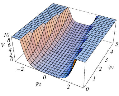
The origin of the tachyonic instability lies in the fact that for non-zero the mass matrix has large off-diagonal terms . Although are small in KL, is not (2i). There is related effect as well: the -field is displaced from the minimum. Even though this displacement is small, as a result the fine-tuned cancellation (tuning at the level in our numerical example) in the KL minimum no longer applies, and can be much larger than it is after inflation. As a result of all this the potential develops an instability, no matter how small the gravitino mass in the post-inflationary vacuum. The effective potential as a function of and with all other fields at their instantaneous minima is shown in figure 1.
The appearance of the instability can be made explicit. As remarked above, is displaced from the post-inflationary minimum. Following [25] to estimate the effect of this we expand the potential during inflation with the post-inflationary minimum. Then
| (2w) |
where we have used that , (the mass matrix is diagonal in ), and we only kept the dominant terms. Minimising the potential with respect to gives
| (2x) |
Using the explicit form for (2u) this evaluates to a potential during inflation with
| (2y) | |||||
with the phase between the two sectors (2r). To get the bottom expression we used relation (2i), and the near degeneracy of the moduli masses. We see the appearance of a destabilising quartic term. The mass becomes tachyonic during inflation when , and the potential develops an instability. It is no use tuning the relative phases to set ; the phase only determines whether it is the displacement of or that gives the largest correction, but its overall size is phase-independent. For the above analysis to be valid, we need , implying . This will hold if the moduli stabilisation scale is much higher than the inflationary scale.
Ref. [4] studied a similar model of SUGRA chaotic inflation combined with a KKLT moduli sector (they set ), and found viable inflation for some parameters. Their model avoids the instabilities coming from the variation of , although only for a narrow range of the ratio . Our results (2w-2y) do not apply to their model because in their case the higher order terms, both and , are not small. However this comes at the cost of fine-tuning. Furthermore, the value of at the KKLT minimum does not satisfy , and so the parameters used are on the borderline of the validity of the model. Even so, this does give a concrete example of how to evade (2w) and its implications. In this paper we are more interested in chaotic inflation models that work for general , without the need for tuning, and will describe such a setup in the next subsection.
To conclude, although the inflaton and modulus sectors can be nearly decoupled in the vacuum after inflation in the KL set-up, this is not true during inflation. The reason is that the (off-diagonal) corrections to the mass matrix are still large, leading to a tachyonic direction in the potential. To see this effect, it is essential to treat the modulus as a dynamical field during inflation. Even though the modulus displacement during inflation is small, it gives a large correction to the inflaton potential which is crucial for a correct analysis of the model.
3.2 Model 1
In this section we discuss model 1 (2n) combined with a moduli sector. As we will see, moduli corrections do not destroy inflation, but give small corrections which are potentially measurable. Comparing with model 2 discussed in the previous section may give further insight into what is needed for a successful inflation model in the presence of moduli.
Including a moduli sector the potential for model 1 (2n), (2r) is with
| (2z) |
with given in (2v). We have set , their values at the minimum during and after inflation in the parameter regime of interest.
The KKLT scenario does not work, due to the usual argument that it is not possible to keep the moduli fixed during inflation while keeping the soft corrections to inflation small. Let us thus concentrate on the fine-tuned KL model. One can calculate the effective potential, taking into account the displacement of during inflation, analogous to (2w)–(2y). The result is similar (note that the effects of all extra terms appearing in in model 1 compared to model 2 give contributions or and are small in the KL set-up):
| (2aa) |
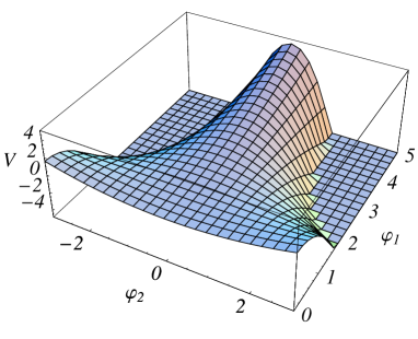
The difference between model 1 and 2 is that in model 1 the field appears explicitly in the Kähler, and consequently receives additional stabilising contributions. This is just enough to keep the -mass positive definite ; the -dependent contribution to the mass from and cancels exactly. A plot of the potential as a function of and all other fields at their instantaneous minimum is shown in figure 1, which confirms that the potential is stable during inflation; the subdominant terms neglected in the analysis (2aa) do not affect the stability.
Thus the moduli sector does not destabilise the inflationary potential, and model 1 provides a viable model of SUGRA chaotic inflation. reduces to the quadratic chaotic inflationary potential in the limit . But is not a minimum during inflation when : . With KL moduli stabilisation the instantaneous minimum of is close to zero. As a result the potential is not exactly quadratic but close to it. To see whether these small deviations are detectable, we have integrated the equations of motion during inflation numerically. The relevant equations are given in A. The results are independent of the initial conditions as long as is large enough for 60 e-folds of inflation; (no shift symmetry) and are heavy and will soon settle in their instantaneous minimum.
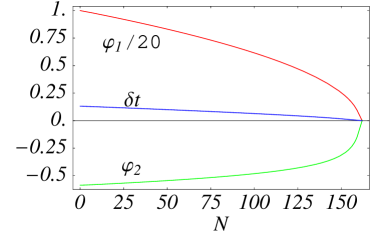
Consider a particular example with parameters . Then from (2g) , and is tuned to get a Minkowski vacuum after inflation. The inflaton mass is set by the COBE normalisation. The field evolution as a function of number of e-folds since the beginning of inflation is shown in figure 4. We started with and the other fields initially at their instantaneous minimum. Inflation ends for , observable scales leave the horizon at , when .
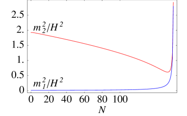
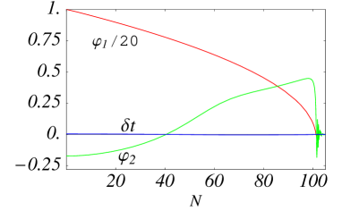
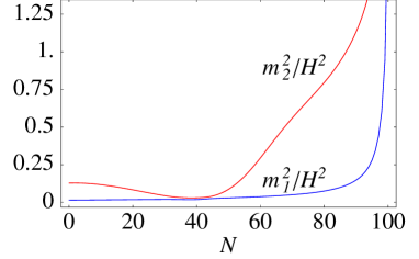
In the vacuum after inflation the inflaton and modulus masses are well separated: , and . The gravitino mass is small as a consequence of small . The hierarchy is preserved during inflation. At COBE scales the modulus mass is , the lowest mass eigenstate (predominantly the shift symmetric with a small admixture of and ) is , while the other inflaton field is heavier . The two inflaton mass eigenstates with are shown in figure 4. The gravitino mass during inflation is .
In all of parameter space (with one exception to be discussed shortly) . Although all fields evolve during inflation, single field inflation is a good approximation. We calculated the slow-roll parameters projected along the inflaton trajectory, and compared them with the usual slow-roll parameter in terms of derivatives of the potential [4, 31, 32, 33]; the difference is less than one percent. See A for the relevant definitions.
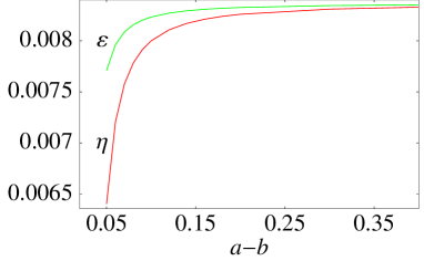
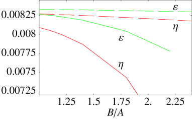
The result for the perturbation spectrum are as follows. The spectral index in all of parameter space is , the same value as in quadratic inflation. The potential is not purely quadratic though. In figure 4 the slow-roll parameters are shown as a function of (the results are fairly independent on absolute scale ). In the limit of large the slow-roll parameters approach as for a purely quadratic potential (2l), but they deviate for small . If tensor perturbations are observed in the future these deviations may be measured, since
| (2ab) |
This breaks the degeneracy between a purely quadratic potential and the current model with small . Figure 4 shows the slow-roll parameters as a function of , for and (lower and upper line). The conclusion is that the deviations from a purely quadratic potential can be large in the limit , and large . This is exactly the limit for which (2h) is large.
The model works for . For larger , i.e. for a modulus sector with larger deviations from the Minkowski SUSY minimum, the mass eigenstates of the inflaton and moduli sector can no longer be separated, and the model is plagued by the same problems as the KKLT set-up. In the region there are parameters for which isocurvature fluctuations can be large. An example is shown in figure 4, for parameters . The reason is that for larger the field crosses the origin during the inflationary evolution. Around the origin the field is light . If this crossing happens around COBE scales, large isocurvature fluctuations are produced. This is the case for our numerical example, where the origin crossing occurs around 60 e-folds before the end of inflation when . The evolution of both the adiabatic and isocurvature perturbation is needed to determine the spectrum; this is beyond the scope of this paper.
4 KL moduli stabilisation and inflation
When can one successfully combine inflation with a fine-tuned KL-style moduli sector (adding their respective superpotentials and only coupling the two sectors gravitationally), and when not? The answer is model dependent but the current discussion has gained some insight. In this section we will expand on this some more.
Consider a model with a Kähler potential
| (2ac) |
The source of instability comes from the terms
| (2ad) |
coupling the modulus and inflaton sector. Although is small during inflation in the KL set-up222In fact can be tuned arbitrarily small by tuning the relative phase between and . However, as discussed in section 3.1 the correction to the potential due to the dynamics of the modulus field is independent of this phase, and thus cannot be tuned., the off-diagonal corrections to the mass matrix are not (2i). As a result, during inflation is slightly displaced from its minimum . Although the displacement is small, it disrupts the minute fine-tuning present in the KL model, and as a result can lead to large corrections to the inflaton potential. This can be made explicit by Taylor expanding around its post-inflationary vacuum [25]. The result is [see (2w)–(2y)] with . The minus sign appears because will adjust to minimise the total potential. The effective inflationary potential is
| (2ae) |
with the potential in the limit that the moduli correction is absent . The correction is potentially large, since , but model dependent. The superpotential could be a series of exponentials, or some polynomial in the inflaton fields. Here we have looked at polynomials, although we expect similar results for both cases. The term corrects the masses of the inflaton sector fields. For successful inflation the correction to the inflaton mass needs to be sufficiently small so that . But in addition we have to make sure the masses of all other fields remain positive definite during inflation, and the potential does not display an instability. All mass corrections automatically vanish if during inflation with running over all inflaton sector fields. This is for example the case in -term hybrid inflation [28, 29, 30]. But in all other cases the mass corrections need to be checked, because as noted, they are large and potentially destructive.
Consider first the case with during inflation; from (2ap) we see that the second term in vanishes, and the effective potential becomes
| (2af) |
where we have allowed for the variation of during inflation, and used (2i). Take a superpotential linear in the inflaton field. The correction term in (2af) then alters the inflaton mass. Introducing a shift symmetry for the inflaton to solve the -problem, the moduli correction can be calculated explicitly. It is too large: . An example is -term hybrid inflation [25]. Thus KL with a linear inflaton superpotential that is non-zero during inflation does not work .
Consider then some polynomial in inflaton sector fields. Now the correction term is a negative quartic or higher order polynomial. As before, inflation requires a sufficiently small inflaton mass ; this is automatic if with the inflaton field. In addition all other “spectator” fields for which should be non-tachyonic during inflation. For the chaotic inflation models discussed in this paper this is achieved if the spectator field appears in , as was the case for model 1. Note that the dominant mass correction to from is the same for all forms of the Kähler. The reason that model 1 is stable and model 2 is not, is simply that the inflaton potential in the former model gives a larger stabilising contribution to the -mass.
We will now consider a model with a more generic Kähler potential, for which is non-zero (2ac), i.e. with the inflaton sector fields appearing inside the log
| (2ag) |
The most stable models are those for which gives the largest mass to . Whether the shift-symmetric inflaton is inside or outside the log does not affect the issue of stability — for simplicity we have put it outside the log in the Kählers above. However, how and where appears is crucial. If has a shift symmetry the potential has an instability during inflation, for , whether appears outside the log in (as in model 2) or inside the log in .
As can be seen from the expressions in B, the form of the different parts of the potential (, etc.) is rather complicated. However we only require their leading order behaviour in . Furthermore, only the dependence part of will contribute significantly to (2x). The relevant terms are then
| (2ah) |
Using the formula (2x), we find , giving
| (2ai) |
independently of . What is rather surprising is that even with does not work. For small the log can be expanded to give . Since model 1 gives a viable model, one would expect to give similar results for . But this is not the case. The inflaton potential differs for and , and thus receives different stabilising mass contributions in each case. It is not enough to expand first, and show that during inflation is small to justify the expansion — analysing the full potential shows an instability.
We see that the placing inside or outside the log is crucial to the success of inflation. Model 1 with outside the log gives a marginally stable model, where the dependent moduli corrections just cancel. As it turns out this is the most stable model. Placing inside the log, no matter what the modular weight is, gives a tachyonic mode.
5 Conclusions
In this paper we studied SUGRA chaotic inflation in the presence of stabilised moduli fields. To avoid the usual -problem a shift symmetry for the inflaton field is introduced. But this is not enough, as the moduli stabilisation sector gives rise to additional contributions to and which are generically not small. The moduli sector breaks supersymmetry, and as a result the inflaton fields get soft mass contributions of the order of the gravitino mass. These corrections need to be small for successful inflation. But in a generic moduli potential such as KKLT, the modulus mass is of the same order as the gravitino mass, and it is impossible to keep the corrections to the inflaton small while making sure the modulus remains fixed in its minimum during inflation. KL addressed this problem by constructing a fine-tuned moduli potential with . Indeed, calculating the potential in any model in which inflation is combined with a KL moduli sector by adding the respective superpotentials, the moduli corrections to inflation appear small while at the same time the modulus is heavy.
All of the above assumes that the modulus is fixed during inflation. However, the modulus is a dynamical field, and this changes the situation drastically. Although during inflation the modulus is only slightly displaced from its post-inflationary vacuum, this is enough to disrupt the minute fine-tuning of the KL model. The corrections to the effective inflaton potential are generically large, and whether inflation works is a model dependent question.
Inflation combined with the KL moduli stabilisation scheme works well if the derivative of the inflaton superpotential during inflation vanishes with running over all inflaton sector fields. This is for example the case for -term hybrid inflation. On the other hand if , there are large corrections to the masses of the inflaton sector fields, which are missed if the modulus dynamics are not kept. For models with a polynomial in the shift symmetric inflaton field, these corrections are fatal. If is some polynomial of inflaton and “spectator” fields, the corrections to the -parameter can be harmlessly small if the spectator fields have a small VEV. However, one must also check that the masses of the spectator fields are positive definite during inflation to avoid a run away behaviour. For the chaotic inflation models under consideration this requires the spectator field to have a minimal Kähler (but note that this model is only “just” stable). It is not sufficient for to appear inside the modulus log with unit modular weight, in which case upon a small field expansion it will have a minimal Kähler. In fact, no matter what the modular weight, if is placed inside the log [see (2ac)] the spectator field becomes tachyonic during inflation.
Our route to a successful inflation model in this paper was to take a specific choice of Kähler potential that minimises the impact of the moduli corrections. We calculated the inflationary predictions for the viable model 1, which has a minimal kinetic term for the spectator field (2n), (2r). Although the spectral index is the same as for chaotic inflation with a quadratic potential, the values of the slow-roll parameters differ from those of a purely quadratic potential. The difference is largest for those parameters that stabilise at large values. The degeneracy between the quadratic model and the model with moduli can be broken if tensor perturbations are observed, as this allows us to extract the values of and from the CMB data. Hence, in the future, with the launch of the Planck satellite, we may be able to observe the presence of moduli fields in the sky.
Note that the problems arising from the variation of the modulus during inflation are not unique to chaotic inflation. Combining moduli with -term hybrid inflation was recently discussed in [34], where even a careful choice of Kähler could not save the model. Instead, taking inspiration from [35], the moduli problems were reduced by multiplying the superpotentials of the two sectors, instead of adding them. It would be interesting to see if a similar approach can help chaotic inflation models, although we will leave this for future work.
Appendix A Perturbations
In this appendix we summarise the relevant equations for the perturbation spectrum.
It is convenient to use the number of e-foldings (normalised so that at the beginning of inflation) as a measure of time. The scales measured by COBE and WMAP leave the horizon e-folds before the end of inflation. As before the subscript denotes the corresponding quantity at COBE scales. Slow-roll inflation ends when one of the slow-roll parameters becomes greater than one. In our numerical analysis we use to determine the end of inflation.
To determine the inflationary trajectory, and the perturbation spectrum, we integrate the equations of motion numerically, using
| (2aj) |
with . Dots indicate derivatives with respect to .
We can define the directional slow-roll parameter as the usual slow-roll parameter projected along the inflaton path [4, 31, 32, 33]:
| (2ak) |
We have checked that in all of parameter space (except for the case with large isocurvature perturbations shown in figure 4) , and inflation is effectively single-field with an adiabatic perturbation spectrum.
The scalar power spectrum is then given by
| (2al) |
evaluated 60 e-folds before the end of inflation. The COBE normalisation imposes that . A second crucial observable is the spectral index of the inflaton fluctuations:
| (2am) |
WMAP3 has measured for a negligible tensor contribution to the perturbation spectrum [36], and for non-zero . We checked that using instead to calculate the spectral index differs by less than a percent from the spectral index (2am) of the adiabatic mode, confirming once again that the usual single field equations apply. The slow-roll parameter is defined as the minimum eigenvalue of the matrix
| (2an) |
where the metric is given by .
Appendix B General Kähler
For a Kähler potential of the form
| (2ao) |
we find that and . The components of the inverse metric are
| (2ap) |
| (2aq) |
where , and
| (2ar) |
For a minimal Kähler , while for a shift symmetry . We see that for all the models considered in this paper, during inflation.
References
References
- [1] A. D. Linde, Chaotic Inflation, Phys. Lett. B 129 (1983) 177
- [2] M. Kawasaki, M. Yamaguchi and T. Yanagida, Natural chaotic inflation in supergravity, Phys. Rev. Lett. 85 (2000) 3572 [hep-ph/0004243]
- [3] K. Kadota and M. Yamaguchi, Phys. Rev. D 76 (2007) 103522 [arXiv:0706.2676 [hep-ph]].
- [4] P. Brax and J. Martin, Shift symmetry and inflation in supergravity, Phys. Rev. D 72 (2005) 023518 [hep-th/0504168]
- [5] R. Kallosh, On Inflation in String Theory, hep-th/0702059
- [6] R. Kallosh and A. Linde, Testing String Theory with CMB, JCAP 0704 (2007) 017 [0704.0647 [hep-th]]
- [7] R. Kallosh, N. Sivanandam and M. Soroush, Axion Inflation and Gravity Waves in String Theory, 0710.3429 [hep-th]
- [8] D. H. Lyth, What would we learn by detecting a gravitational wave signal in the cosmic microwave background anisotropy?, Phys. Rev. Lett. 78 (1997) 1861 [hep-ph/9606387]
- [9] K. Freese, J. A. Frieman and A. V. Olinto, Natural inflation with pseudo - Nambu-Goldstone bosons, Phys. Rev. Lett. 65 (1990) 3233
- [10] D. Baumann and L. McAllister, A microscopic limit on gravitational waves from D-brane inflation, Phys. Rev. D 75 (2007) 123508 [hep-th/0610285]
- [11] R. Bean, S. E. Shandera, S. H. Henry Tye and J. Xu, Comparing Brane Inflation to WMAP, JCAP 0705 (2007) 004 [hep-th/0702107]
- [12] S. Dimopoulos, S. Kachru, J. McGreevy and J. G. Wacker, N-flation, hep-th/0507205
- [13] T. W. Grimm, Axion Inflation in Type II String Theory, 0710.3883 [hep-th]
- [14] A. R. Liddle, A. Mazumdar and F. E. Schunck, Assisted inflation, Phys. Rev. D 58 (1998) 061301 [astro-ph/9804177]
- [15] E. J. Copeland, A. R. Liddle, D. H. Lyth, E. D. Stewart and D. Wands, False vacuum inflation with Einstein gravity, Phys. Rev. D 49 (1994) 6410 [astro-ph/9401011]
- [16] M. Dine, L. Randall and S. D. Thomas, Supersymmetry breaking in the early universe, Phys. Rev. Lett. 75 (1995) 398 [hep-ph/9503303]
- [17] M. K. Gaillard, D. H. Lyth and H. Murayama, Inflation and flat directions in modular invariant superstring effective theories, Phys. Rev. D 58 (1998) 123505 [hep-th/9806157]
- [18] T. Banks, M. Berkooz, S. H. Shenker, G. W. Moore and P. J. Steinhardt, Modular Cosmology, Phys. Rev. D 52 (1995) 3548 [hep-th/9503114]
- [19] R. Kallosh and A. Linde, Landscape, the scale of SUSY breaking, and inflation, JHEP 0412 (2004) 004 [hep-th/0411011]
- [20] S. Kachru, R. Kallosh, A. Linde and S. P. Trivedi, De Sitter vacua in string theory, Phys. Rev. D 68, 046005 (2003) [hep-th/0301240]
- [21] S. B. Giddings, S. Kachru and J. Polchinski, Hierarchies from fluxes in string compactifications, Phys. Rev. D 66 (2002) 106006 [hep-th/0105097]
- [22] C. P. Burgess, R. Kallosh and F. Quevedo, de Sitter string vacua from supersymmetric D-terms, JHEP 0310 (2003) 056 [hep-th/0309187]
- [23] A. Achucarro, B. de Carlos, J. A. Casas and L. Doplicher, de Sitter vacua from uplifting D-terms in effective supergravities from realistic strings, JHEP 0606 (2006) 014 [hep-th/0601190]
- [24] M. Gomez-Reino and C. A. Scrucca, Locally stable non-supersymmetric Minkowski vacua in supergravity, JHEP 0605 (2006) 015 [hep-th/0602246]
- [25] P. Brax, C. van de Bruck, A. C. Davis and S. C. Davis, Coupling hybrid inflation to moduli, JCAP 0609 (2006) 012 [hep-th/0606140]
- [26] L. O’Raifeartaigh, Spontaneous Symmetry Breaking For Chiral Scalar Superfields, Nucl. Phys. B 96 (1975) 331
- [27] A. Chambers and A. Rajantie, Lattice calculation of non-Gaussianity from preheating, 0710.4133 [astro-ph]
- [28] E. Halyo, Hybrid inflation from supergravity D-terms, Phys. Lett. B 387 (1996) 43 [hep-ph/9606423]
- [29] P. Binetruy and G. R. Dvali, D-term inflation, Phys. Lett. B 388 (1996) 241 [hep-ph/9606342]
- [30] Ph. Brax, C. van de Bruck, A. C. Davis, S. C. Davis, R. Jeannerot and M. Postma, Moduli corrections to D-term inflation, JCAP 0701 (2007) 026 [hep-th/0610195]
- [31] C. Gordon, D. Wands, B. A. Bassett and R. Maartens, Phys. Rev. D 63 (2001) 023506 [arXiv:astro-ph/0009131].
- [32] S. Groot Nibbelink and B. J. W. van Tent, Class. Quant. Grav. 19 (2002) 613 [arXiv:hep-ph/0107272].
- [33] B. J. W. van Tent, Class. Quant. Grav. 21 (2004) 349 [arXiv:astro-ph/0307048].
- [34] S. C. Davis and M. Postma, Successfully combining SUGRA hybrid inflation and moduli stabilisation, 0801.2116 [hep-th]
- [35] A. Achúcarro and K. Sousa, F-term uplifting and moduli stabilization consistent with Kahler invariance, 0712.3460 [hep-th]
- [36] D. N. Spergel et al. [WMAP Collaboration], Wilkinson Microwave Anisotropy Probe (WMAP) three year results: Implications for cosmology, Astrophys. J. Suppl. 170 (2007) 377 [astro-ph/0603449]