Hydrodynamical adaptive mesh refinement simulations of turbulent flows - I. Substructure in a wind

Abstract

The problem of the resolution of turbulent flows in adaptive mesh refinement (AMR) simulations is investigated by means of 3D hydrodynamical simulations in an idealised setup, representing a moving subcluster during a merger event. AMR simulations performed with the usual refinement criteria based on local gradients of selected variables do not properly resolve the production of turbulence downstream of the cluster. Therefore we apply novel AMR criteria which are optimised to follow the evolution of a turbulent flow. We demonstrate that these criteria provide a better resolution of the flow past the subcluster, allowing us to follow the onset of the shear instability, the evolution of the turbulent wake and the subsequent back-reaction on the subcluster core morphology. We discuss some implications for the modelling of cluster cold fronts.

1 Introduction

The role of turbulence in astrophysics and, in particular, in cosmic structure formation has been attracting increasing attention, along with observational and theoretical indications of its relevance. There are different observational hints converging towards the turbulent character of the intra-cluster medium (ICM) (Schuecker et al. 2004; Churazov et al. 2004; Enßlin & Vogt 2006; Rebusco et al. 2005, 2006, but see also Fabian et al. 2003). From an observational point of view, the next generation of X-ray observatories will be able to observe the Doppler shifts of emission lines of heavy ions due to bulk motions in the ICM, thus providing information about the turbulent state of the flow. Numerical studies predict that gas bulk motions and turbulence in the ICM can be a consequence of cluster merging (Ricker, 1998; Norman & Bryan, 1999; Takizawa, 2000; Ricker & Sarazin, 2001; Dolag et al., 2005). In their model, Subramanian et al. (2006) identify three physical regimes for turbulence production and decay in clusters, the latest one being dominated by turbulent production in the wakes of minor mergers. This phase would play a key role also for the magnetic field amplification in the ICM.

Merging is a crucial process in cosmic structure formation. It is predicted in the framework of hierarchical clustering and can be studied theoretically by means of numerical simulations (e.g. Roettiger et al. 1996, 1998; McCarthy et al. 2007). Observationally, modern X-ray observatories are able to detect substructures in the ICM that are indicative of merging (Sunyaev et al., 2003). Among the first results of galaxy cluster observations with Chandra was the discovery of “cold fronts” in the merging clusters A2142 and A3667, and later in many other clusters (see Markevitch & Vikhlinin 2007 for a review). The origin of cold fronts in merger clusters has been ascribed to infalling substructures, although the cold fronts in the cores of cooling core clusters have a different interpretation (Tittley & Henriksen, 2005; Ascasibar & Markevitch, 2006).

Cosmological simulations of galaxy cluster formation have confirmed the merging scenario for the transient formation of cold fronts (Bialek et al., 2002; Nagai & Kravtsov, 2003). The problem has also been addressed with simplified setups, which allow a better control over the involved physical parameters, in 2D (Acreman et al., 2003; Heinz et al., 2003; Asai et al., 2004; Xiang et al., 2007) and 3D simulations (Takizawa, 2005a, b; Asai et al., 2005, 2007; Dursi & Pfrommer, 2008).

The theoretical study of turbulence in the framework of full cosmological simulations is a challenging task and presents the typical problems of numerical simulations of strongly clumped media. Adaptive mesh refinement (AMR) is a viable tool for saving computational resources and modelling the large dynamic range in a proper way (Norman, 2005). The choice of the most suitable mesh refinement criterion is thus a delicate compromise between following the flow structure in the most accurate way and exploiting the advantage of saving computational time and memory.

This study (Paper I) is the first part of a broader project on the physics of galaxy clusters, focused on investigating the generation of turbulence in the ICM by means of AMR simulations. In Paper I, we present new AMR criteria that are more suitable for resolving the production of turbulence than those commonly used in cosmological simulations. They were tested in a simple setup, reminiscent of a wind tube experiment, but designed in order to be representative of an idealised subcluster merger. This test problem is a useful and controlled testbed for the new tools, far from the complexity of a more realistic cosmological simulation. Nevertheless, it is similar to previous studies of subcluster mergers and can provide useful insights about the physics of the minor mergers, relevant for the generation of turbulence in the ICM. In contrast with earlier work, we focus our analysis on the turbulent wake of the subcluster rather than on the cold front, showing the difference of the evolution of the Kelvin-Helmholtz instability (KHI) resulting from the use of different AMR criteria.

The second step, described in Iapichino & Niemeyer (2008) (hereafter Paper II), is to apply the same tools to simulations of structure formation and to study the turbulent flow in the ICM. The results of the present work will thus be compared with the outcomes of more realistic simulations of minor mergers.

The paper is structured as follows: the new refinement criteria are defined in in Sec. 2. The numerical setup of the performed simulations and the features of the KHI are introduced in Sects. 3 and 4, respectively. The results are presented in Sec. 5 and discussed in Sec. 6.

2 Refinement criteria and resolution of turbulent flows

Three different AMR criteria are used in the simulations discussed in this work. A rather general and widely used criterion is based on the local gradients of all thermodynamical variables. If the relative slope $|(q(i+1)-q(i-1))/q(i)|$ of a variable $q$ in a cell $i$ is larger than a given threshold, that cell is marked for refinement. Numerical tests showed that, for our subcluster problem, this criterion quickly leads to a high level of refinement in the entire computational domain. This shortcoming was fixed by allowing the refinement on the local gradients of only selected variables. The AMR criterion named “1” in our work is based on the local gradients of density and internal energy, with thresholds $0.24$ and $0.25$ respectively, tuned for optimal performance.

Two novel AMR criteria, developed for tracking the evolution of a turbulent flow (Schmidt et al., 2008), were tested in this study. In both cases, the control variables for refinement are given by scalars probing small-scale features of the flow. One example is the modulus of the vorticity vector $\mn@boldsymbol{\omega}=\nabla\times\mn@boldsymbol{v}$ (the curl of the velocity field) that is expected to become high in regions filled by turbulent eddies. In addition, the mechanism for triggering refinement has been modified. Rather than normalising the control variables in terms of characteristic quantities and comparing to prescribed threshold values, the new criteria use regional thresholds for triggering refinement which are based on a comparison of the cell value of the variable $q(\mn@boldsymbol{x},t)$ with the average and the standard deviation of $q$, calculated on a local grid patch:

$$q(\mn@boldsymbol{x},t)\geq\langle q\rangle_{i}(t)+\alpha\lambda_{i}(t)$$ (1)

where $\lambda_{i}$ is the maximum between the average $\langle q\rangle$ and the standard deviation of $q$ in the grid patch $i$, and $\alpha$ is a tunable parameter. This technique can easily handle highly inhomogeneous problems such as subcluster mergers without a priori knowledge of the flow properties.

We define criterion “2” using the square of the vorticity, $\omega^{2}$, as the control variable. Refining upon criterion “2” only, one can expect to resolve turbulent eddies which are associated with high vorticity but not flow features arising from pure compression such as shock fronts. For this reason, in criterion “3”, the control variable is given by the rate of compression, i.e., the negative time derivative of the divergence $d=\nabla\cdot\mn@boldsymbol{v}$. In combination with refinement by vorticity, this criterion is intended to refine flow regions in which steep density gradients are developing. One could also refine by $-d$ or $d^{2}$ in order to capture compression effects. However, this would give rise to full refinement of highly compressed gas, despite the fact that the interiors of compressed regions do not necessarily exhibit rich small-scale structure. Maxima of the rate of compression, on the other hand, are typically found at the interfaces between dense and rarefied gas. As we have seen in applications, a drawback of criterion “3” is that refinement can be triggered prematurely in some instances. This undesired side-effect can be suppressed by introducing a lower cutoff for the refinement thresholds.

3 Numerical simulations

Table 1: Scheme of the performed simulations.

Simulation	number of AMR levels	AMR criterion
$A$	5	1
$B$	4	1
$C$	6	1
$D$	5	2
$E$	5	2+3

The list of the performed calculations is reported in Table 1. In the first column, the simulations are identified by a letter. The second column reports the number $n$ of AMR levels which are allowed in the simulation. The root grid resolution of the runs is only $16^{3}$ but the effective resolution is finer because AMR is used. The refinement factor is 2, thus the effective resolution is $(16\times 2^{n})^{3}$ grid cells. In the standard case of five additional AMR levels, the effective resolution is therefore $(16\times 2^{5})^{3}=512^{3}$ grid elements.

The third column of Table 1 indicates which criterion was used for performing the grid refinement, according to the definitions of Sec. 2. The simulations $A$, $B$ and $C$ make use of criterion “1” in a resolution study, whereas the simulations $D$ and $E$ were performed with the novel AMR criteria “2” with threshold $\alpha_{2}=0.2$, and “$2+3$” with $\alpha_{2}=1.0$, $\alpha_{3}=2.0$, respectively.

The 3D simulations were performed using the AMR, grid-based hybrid (hydrodynamical plus N-Body) code enzo (O’Shea et al., 2005), with the N-Body section of the code switched off. The primary hydrodynamic method used in enzo is based on the piecewise parabolic method (PPM) (Woodward & Colella, 1984), modified for the study of cosmology (Bryan et al., 1995). Also available is the hydrodynamic finite-difference algorithm of the zeus code (Stone & Norman, 1992a, b), used for tests in Sec. 5.3.1.

Since we assumed ideal adiabatic physics for our calculations, the simulations are scale-free and all quantities were rescaled to get numbers of the order unity, as shown in Robinson et al. (2004). However, for the sake of clarity, all quantities are reported in CGS units. An adiabatic equation of state was used, with $\gamma=5/3$.

In the initial conditions, an isothermal and spherical symmetric object is set in the computational domain according to a beta density profile (Cavaliere & Fusco-Femiano, 1978):

$$\rho(r)=\rho_{\mathrm{c}}\left[1+\left(\frac{r}{r_{\mathrm{c}}}\right)^{2}\right]^{-3\beta/2}\,\,,$$ (2)

where $\rho$ is the gas density, $r$ is the distance from the centre, $\rho_{\mathrm{c}}$ is the central density, and $r_{\mathrm{c}}$ is the core radius. The most important difference between this setup and a typical wind tube experiment (cf. Murray et al. 1993; Vietri et al. 1997; Agertz et al. 2007) is the presence of gravity. The gravitational acceleration is provided by a fixed spherical dark matter distribution following a King profile,

$$\rho_{\mathrm{DM}}(r)=\rho_{\mathrm{DM,c}}\left[1+\left(\frac{r}{r_{\mathrm{c}}}\right)^{2}\right]^{-3/2}\,\,,$$ (3)

with $\rho_{\mathrm{DM,c}}=10\ \rho_{\mathrm{c}}$. A cutoff was set at $r=5\ r_{\mathrm{c}}$, both for the dark matter density profile and the gravitational acceleration (cf.  Takizawa, 2005a). Given the King profile for the dark matter component of an isothermal cluster, the beta profile is the hydrostatic equilibrium solution for the gas density. The hydrostatic equilibrium is enforced on the discrete computational grid by the relaxation procedure of the initial state described by Zingale et al. (2002).

The interaction of the subcluster with a background wind mimics the merger process in a simplified manner. A uniform velocity field along the $x$-axis is imposed in the background medium. In this simplified setup, we implicitly assume that the merging process has a negligible impact on the dark matter density profile of the subcluster.

The numerical values of the parameters defined above were chosen as typical of a subcluster merger. We set $\rho_{\mathrm{c}}=6.3\times 10^{-27}\ \mathrm{g\ cm^{-3}}$, $r_{\mathrm{c}}=7.7\times 10^{23}\ \mathrm{cm}=250\ \mathrm{kpc}$ and $\beta=0.6$, which result in a subcluster temperature $kT=3.65\ \mathrm{keV}$. The background medium has constant values of density $\rho_{\mathrm{b}}=7.9\times 10^{-28}\ \mathrm{g\ cm^{-3}}$ and temperature $kT_{\mathrm{b}}=8.0\ \mathrm{keV}$. The background velocity is chosen as $v_{\mathrm{b}}=1.6\times 10^{3}\ \mathrm{km\ s^{-1}}$, $v_{\mathrm{b}}/c_{\mathrm{b}}=1.1$, where $c_{\mathrm{b}}$ is the sound speed of the background. The interface between the subcluster and the uniform medium is defined at the locations where the subcluster and background gas pressures are equal.

The computational domain has a size of $[0,4\ \mathrm{Mpc}]^{3}$, meaning that the effective resolution of $512^{3}$ corresponds to an effective spatial resolution of $7.8\ \mathrm{kpc}$. The boundary conditions are inflowing at the left $x$-boundary and outflowing elsewhere. The subcluster is initially resolved with the finest AMR level available, in order to minimise any mapping errors related to the hydrostatic equilibrium of the initial state.

4 The Kelvin-Helmholtz instability

The simulations are carried out in the rest frame of the subcluster, set at rest in a moving background medium. The outer subcluster interface is thus subject to the Kelvin-Helmholtz instability. If gravity is neglected, the KHI may grow for all values of wavenumber $k$. The linear growth timescale of the KHI, in the case of a flat interface between two incompressible fluids of different densities, is (Drazin & Reid 2004; cf. Agertz et al. 2007):

$$\tau_{\mathrm{KH}}=\frac{2\pi(\rho_{\mathrm{1}}+\rho_{\mathrm{2}})}{k(\rho_{\mathrm{1}}\rho_{\mathrm{2}})^{1/2}V}$$ (4)

The geometry of the subcluster is different from this idealised case, but an order-of-magnitude estimate of $\tau_{\mathrm{KH}}$ can be obtained by setting $\rho_{\mathrm{1}}=0.3\,\rho_{\mathrm{c}}$ (subcluster density at the interface with the background medium), $\rho_{\mathrm{2}}=\rho_{\mathrm{b}}$, $k=2\pi/R$, where $R\sim 1.7\,r_{\mathrm{c}}$ is the distance from the subcluster centre to the interface with the background medium. The velocity $V$ is smaller than $v_{\mathrm{b}}$ because a bow shock forms in front of the subcluster and $V$ has to be determined from the post-shock conditions (cf. Agertz et al. 2007). For this rough estimate it is adequate to assume $V\approx 0.7\,v_{\mathrm{b}}$ (also in agreement with the simulations). With these choices, $\tau_{\mathrm{KH}}\approx 0.8\ \mathrm{Gyr}$. This is an estimate of the time required to the KHI to perturb the spherical shape of the subcluster substantially. We set the total simulation time to $4\ \mathrm{Gyr}$.

The previous timescale analysis motivates the choice of neglecting radiative cooling in the performed simulations. The effect of cooling is not expected to be prominent because both for the subcluster and the background medium the cooling timescale is about two times longer than the total simulation time, and much longer than $\tau_{\mathrm{KH}}$.

The presence of the gravitational acceleration stabilises a perturbation of wavenumber $k$ if (Paterson 1984; cf. Murray et al. 1993)

$$g\ga\frac{\rho_{\mathrm{1}}\rho_{\mathrm{2}}V^{2}k}{\rho_{\mathrm{1}}^{2}-\rho_{\mathrm{2}}^{2}}$$ (5)

where $g$ is the modulus of the gravitational acceleration at the interface. In the subcluster case, this stabilisation only affects wave numbers that are much smaller than $2\pi/R$. Gravity thus fails to stabilise the subcluster against the KHI.

The loss of gas from the subcluster atmosphere due to the ram pressure of the background flow, discussed by Heinz et al. (2003), is not effective for our choice of parameters. The gas stripping and its subsequent mixing into the ambient medium is instead caused by the KHI, and will be described in Sect. 5.3.

5 Results

5.1 Evolution of the subcluster

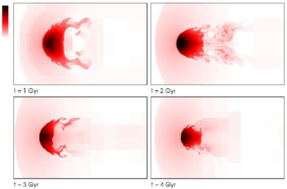
Figure 1: Density slices ($xz$ plane) of a part of the computational domain ($2.6\times 1.6\ \mathrm{Mpc}$), showing the subcluster evolution at different times, for the run $A$. The density is linearly colour coded, following the colour bar on the upper left. Time is indicated at the lower left of each panel.

The morphological evolution of the idealised subcluster is shown in the four density slices of Fig. 1. The figure refers to run $A$, which (as discussed in Sec. 5.2) has a suitable spatial resolution for our problem.

At $t=1\ \mathrm{Gyr}$, a bow shock has formed in front of the subcluster and the KHI is growing at the sides. At $t=2\ \mathrm{Gyr}$ a turbulent, eddy-like flow in the subcluster wake is clearly visible. Yet it is not resolved at later times, as will be discussed in Sec. 5.3. The KHI leads to mass stripping in the subcluster, which will be quantified in Sect. 5.2.

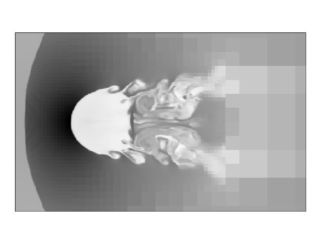
Figure 2: Temperature slice ($xz$ plane) of the subcluster at $t=2\ \mathrm{Gyr}$ for the run $A$ (AMR on gradients of density and internal energy). The temperature is linearly colour coded in gray-scale.

From $t=2\ \mathrm{Gyr}$, the morphology which is visible at the left interface of the subcluster (Fig. 2) closely resembles a typical cold front structure. Based on Chandra observations of A3667, Vikhlinin et al. (2001a, b) and Vikhlinin & Markevitch (2002) state that the very existence of the cold fronts requires the suppression of the KHI and of the thermal conduction at the interface between the subcluster gas and the ICM, likely caused by the presence magnetic fields. The MHD simulations of Asai et al. (2004), Asai et al. (2005) and Asai et al. (2007) include anisotropic thermal conduction and show an effective stabilisation of the cold front. The suppression of the thermal conduction is needed to reproduce the observed temperature profiles of the cold front in A3667 in the SPH simulations of Xiang et al. (2007).

Our simulations include neither heat conduction nor magnetic fields. Similar to Heinz et al. (2003), a “cold front-like” structure is thus visible but, according to the above cited simulations, it does not catch the physics of the astrophysical problem. However, its analysis is not the primary goal of this work. In Sec. 6, we will extend the discussion of the subcluster evolution to examples which take into account such additional physics.

5.2 Resolution study

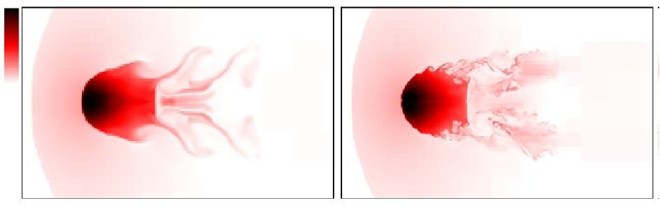
Figure 3: Density slices of the subcluster at $t=2\ \mathrm{Gyr}$ (cf. Fig. 1, upper right panel), in simulations with different effective resolution. Left: run $B$. Right: run $C$. The density is linearly colour coded, according to the colour bar on the left.

A comparison of AMR runs with different resolution is useful for understanding how effectively (or not) the idealised subcluster is modelled in the simulations. With this intent, besides the presented run $A$ we performed the additional runs $B$ and $C$ (cf. Table 1), which implement the same AMR criterion as $A$ and have the same root grid resolution, but allow different numbers of additional AMR levels. Figure 3 permits a morphological comparison at $t=2\ \mathrm{Gyr}$. The run $B$ allows four additional levels of refinement and has a lower effective resolution than run $A$. Comparing Fig. 3, left, and the upper right panel of Fig. 1, a less developed shear instability and an almost regular pattern in the flow at the subcluster tail is noticeable in the former. The crucial features of the subcluster evolution are therefore not properly followed at this level of resolution. On the other hand, the analysis of more resolved run $C$ (six additional AMR levels) shows obviously a better resolution than run $A$ and an enhanced development of the KHI at the sides of the subcluster. Nevertheless, it does not provide any new element for the study of the problem, and therefore the effective resolution of the run $A$ is considered to be adequate for our investigation.

Figure 4: Temporal evolution of subcluster baryonic mass fraction for the runs $A$ (solid line), $B$ (dotted line) and $C$ (dashed line). The mass fraction is normalised to its value at $t=0\ \mathrm{Gyr}$.

A more quantitative comparison is obtained by defining a diagnostic of gas stripping resulting from the development of the KHI. A suitable quantity is adapted from the “cloud mass fraction” defined by Agertz et al. (2007), hence we consider the gas with $T<0.9\ T_{\mathrm{b}}$ and $\rho>0.32\ \rho_{\mathrm{c}}$ as belonging to the subcluster. After a transient phase related to the development of the bow shock, where the “subcluster mass” seems to increase, this quantity (Fig. 4) decreases with time. Similar to Agertz et al. (2007), the subcluster stripping is more pronounced in the more resolved runs, due to the better resolved small scale instability and mixing.

5.3 AMR study

One of the most interesting features of the subcluster evolution in run $A$ is the loss of resolution in the wake at late times. This is an effect of the AMR criterion chosen in that simulation, which cannot effectively refine the turbulent tail (or, at least, without wasting the advantage of AMR, with unnecessary refinement in almost the entire computational domain).

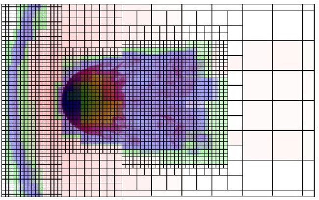
Figure 5: Density slice as in Fig. 1, upper right panel, with the mesh structure superimposed. Grids of AMR levels from 0 to 3 are rendered as mesh structures, whereas for ease of visualisation grids of level 4 and 5 are only rendered with colours green and blue, respectively.

In a study of cold front physics, one could think that the refinement of run $A$ (Fig. 5) is acceptable, because the attention is focused on the better resolved part of the computational domain. We dispute this statement in this section. To this aim, we checked whether alternative AMR criteria can better track the turbulent wake, provided the rest of the cluster morphology is also appropriately refined.

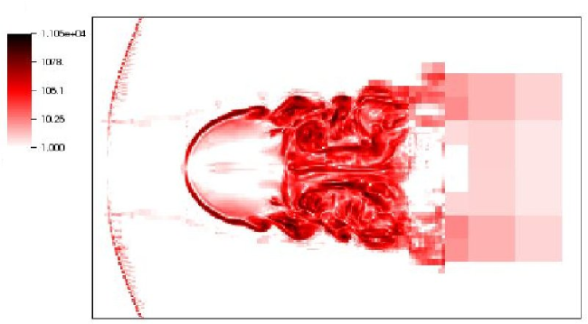
Figure 6: Slice of the subcluster at $t=2\ \mathrm{Gyr}$ for the run $A$ (cf. Fig. 1, upper right panel), showing the square of the vorticity modulus $\omega^{2}$. The quantity is colour coded on a logarithmic scale in code units.

Velocity fluctuations at all scales are the prominent feature of a turbulent flow. It suggests that quantities related to the spatial derivatives of velocity can be particularly suitable for the characterisation of the flow. Figure 6, which shows a slice of the square of the vorticity modulus in run $A$, clearly confirms this idea: the morphology of the turbulent flow is well tracked in comparison with the less contrasted density and temperature eddies, which are not very suitable for triggering the mesh refinement.

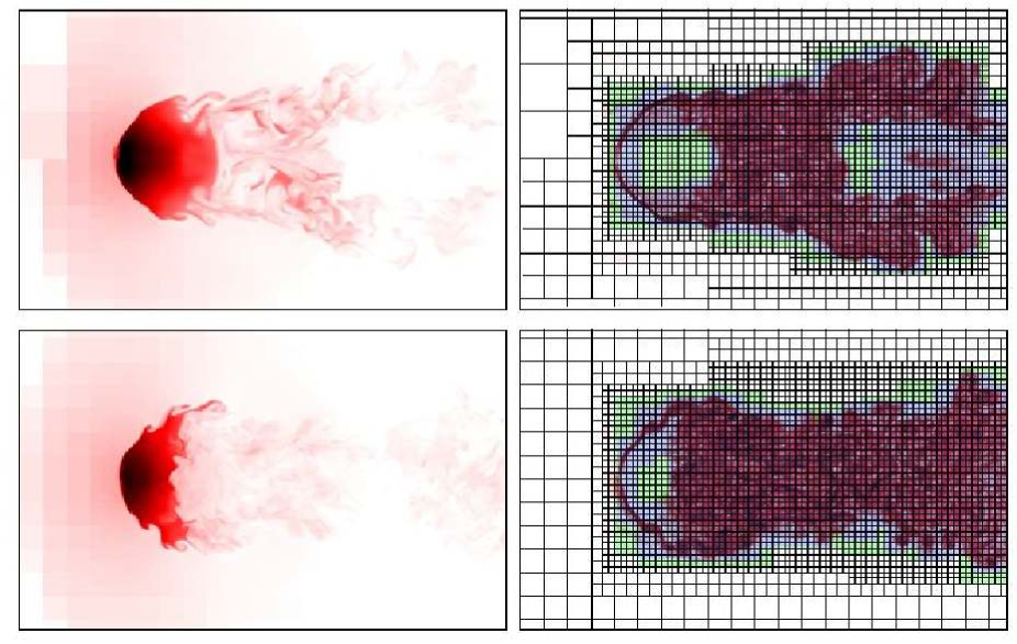
Figure 7: Slices ($xz$ plane) for the run $D$, showing density (left) and square of the vorticity modulus, with the mesh superimposed and visualised according to the rendering used in Fig. 5 (right). Upper panels: slices $t=2\ \mathrm{Gyr}$. Lower panels: slices $t=3\ \mathrm{Gyr}$.

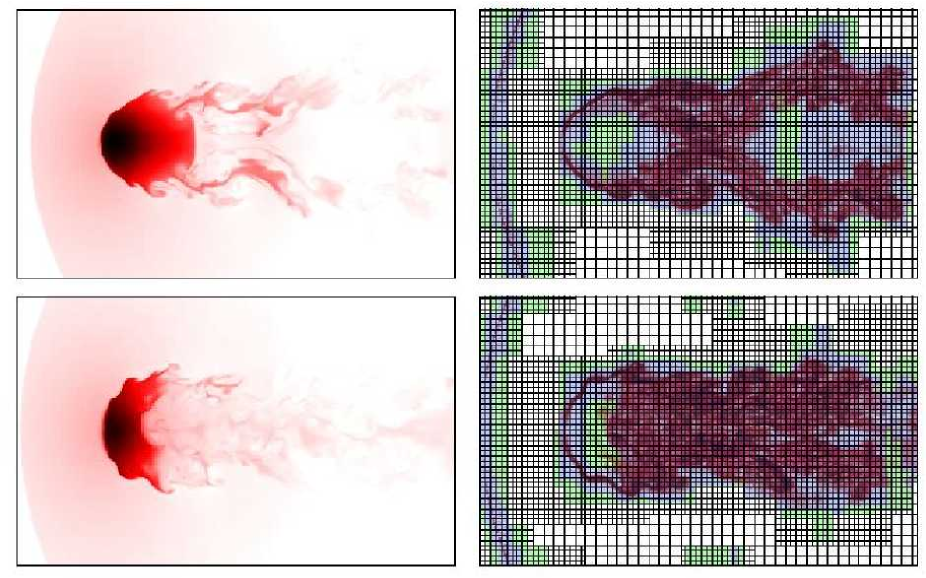
Figure 8: Same as Fig. 7, for run $E$.

The refinement criteria “2” and “3”, presented in Sect. 2, are based on this concept. Their effect on the resolution of the turbulent subcluster wake can be evaluated by the analysis of the runs $D$ and $E$ (Figs. 7 and 8, respectively, at $t=2$ and $3\ \mathrm{Gyr}$). From the density and vorticity slices one can immediately recognise that, in both simulations, the subcluster wake is effectively resolved down to the finest available AMR levels. Moving out of the subcluster, the refinement level decreases gradually.

A closer look reveals that there are some differences between the two simulations. As anticipated in Sec. 2, the refinement criterion “2” alone is unable to resolve the bow shock in front of the subcluster at the finest levels of refinement (run $D$). It is difficult to state whether this has any effect on the development of the KHI, but it is certainly not desirable to underresolve such an important feature of the problem, well resolved in run $E$.

The subcluster tail in run $E$ at $t=2\ \mathrm{Gyr}$ (Fig. 8, upper left) has a more filamentary pattern, intriguingly similar to the more resolved run $C$ (cf. Fig. 3, right).

At $t=3\ \mathrm{Gyr}$, in both runs $D$ and $E$ the subcluster appears more perturbed and prone to the KHI than run $A$ (Fig. 1, lower left panel). Since the subcluster front is well resolved with the refinement criteria used in all simulations, this difference is (at least partly) to be ascribed to the back-reaction of the tail. The turbulent eddies in the subcluster wake are better resolved in runs $D$ and $E$, and partly disturb the morphology of the subcluster core even though it is well resolved. This effect of back-flow is rather similar to that described by Heinz et al. (2003), which identify the displacement of the subcluster core with respect to the potential well as an additional source.

Figure 9: Detail of the temporal evolution of normalised subcluster mass fraction for the runs $A$ (solid line), $C$ (dotted line), $D$ (dashed line) and $E$ (dot-dashed line).

As a measure of the action of the KHI, the subcluster mass has been introduced in Sec. 5.2. It is useful to investigate quantitatively the effect of the back-flow, comparing the time evolution of this quantity in the runs $A$, $C$, $D$, and $E$ (Fig.9). Interestingly, after $t=2\ \mathrm{Gyr}$ the stripping for the runs $D$ and $E$ is more effective than for the run $A$, and follows more closely the curve of the more resolved run $C$. The seeming analogy comes from the convergence of two different features of the small-scale mixing, which for run $C$ is more active at the sides of the subcluster, whereas for the runs $D$ and $E$ is triggered mainly by the tail back-flow.

Table 2: Mass-weighted rms velocity in the test volume of $(400\ \mathrm{kpc})^{3}$, at $t=3\ \mathrm{Gyr}$. The run labelled as “Static” will be introduced in Sect. 5.3.2.

run	$v_{\mathrm{rms}}\ (\mathrm{km\ s^{-1}})$
$A$	260
$D$	530
$E$	530
Static	620

In order to further quantify the effectiveness of the tested AMR criteria, the mass-weighted root mean squared (rms) velocity $v_{\mathrm{rms}}$ is calculated in a test volume of $(400\ \mathrm{kpc})^{3}$, located immediately downstream of the subcluster, at $t=3\ \mathrm{Gyr}$ (Table 2). The simulations using the novel AMR criteria are able to get much higher turbulent velocities than run $A$. These values are in the range predicted theoretically (Subramanian et al., 2006) and found numerically in similar works (Acreman et al., 2003; Takizawa, 2005a, b). Interestingly, the new AMR criteria bring $v_{\mathrm{rms}}$ close to the value which is obtained by an equivalent static grid simulation (cf. Sect. 5.3.2).

A closer analysis of the subcluster tail shows that, at a distance from the subcluster core $r\approx 5\ r_{\mathrm{c}}$, the density structure slightly loses contrast. This is an artifact introduced by the cutoff in the dark matter density and gravitational acceleration (Sect. 3). We tested that the results are not harmed by this shortcoming. Moreover, the vorticity pattern is basically not affected by the cutoff (Figs. 7 and 8) and the same is true for the new refinement criteria.

Table 3: Occupation fraction of the AMR levels at $t=2\ \mathrm{Gyr}$, for the runs $A$, $D$ and $E$ (the AMR level 0 corresponds to the root grid). The fraction is normalised to the whole computational domain. For computational efficiency, in all simulations the refinement is allowed only in the region of interest around the subcluster, with a volume fraction 0.608.

AMR level	run $A$	run $D$	run $E$
1	0.150	0.156	0.422
2	0.100	0.076	0.255
3	0.052	0.045	0.126
4	0.027	0.031	0.074
5	0.015	0.022	0.045

From the point of view of the AMR performance, Table 3 summarises the volume occupation fractions at different levels for three of the runs under examination, at $t=2\ \mathrm{Gyr}$. As expected, the simulations $D$ and $E$ have larger occupation fractions than run $A$. In all cases, the ratio between the occupation fractions at levels $n$ and $n+1$ lies between 1.4 and 2.0, and only a small fraction of the computational domain is refined at the higher levels. Though the overall quality of the AMR operation seems thus acceptable, a visual inspection of Fig. 7 and 8, right panels, shows that a more efficient use of refinement is made in run $D$ than in run $E$. The latter refines the front bow shock better than the former but, despite of the implemented refinement cutoff, it triggers some spurious grids at the sides of the subcluster. This issue is not severe and is perfectly manageable within the available computational resources. In a general sense, this is a good example of tuning AMR to specific problems, finding a difficult equilibrium between a accurate description of the flow and a convenient use of the tool.

5.3.1 Comparison with results from the zeus solver

It is well known that the simulation of the development of hydrodynamical instabilities and the onset of turbulence depends sensitively on the adopted numerical scheme. This issue is extensively addressed by Agertz et al. (2007), in a simulation setup which differs from ours only for the role of gravity, and for the density profile of the subcluster. A similar, detailed study of our setup is out of the scope of this paper, but we performed a simulation similar to run $A$ (5 AMR levels, AMR criterion “1”) using the zeus solver available in enzo (cf. Stone & Norman 1992a, b) instead of PPM. The use of enzo with this solver has been tested by Agertz et al. (2007) in static grid simulations, whereas here it is applied to an AMR run.

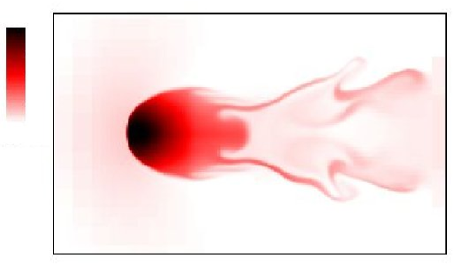
Figure 10: Density slice of the subcluster at $t=2\ \mathrm{Gyr}$ (cf. Fig. 1, upper right panel), in the simulation with the AMR parameters as in run $A$, but using the zeus solver of enzo. The density is linearly colour coded following the colour bar on the left.

Figure 11: Temporal evolution of subcluster baryonic mass fraction for the runs $A$ (solid line) and the run using the zeus solver (dotted line). The mass fraction is normalised to its value at $t=0\ \mathrm{Gyr}$.

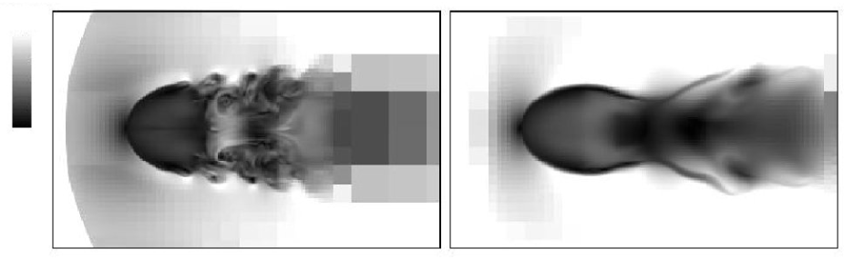
Figure 12: Slices of the subcluster at $t=2\ \mathrm{Gyr}$ (cf. Fig. 1, upper right panel), showing the velocity magnitude. Left: run $A$. Right: run using the zeus solver. The velocity magnitude is linearly coded such that that the colour-bar ranges from $v=0$ (black) to the imposed background velocity ($v=1.6\times 10^{3}\ \mathrm{km\ s^{-1}}$, white).

The results of this simulation show clearly that the zeus solver is unable to follow the onset of the KHI and the subsequent development of turbulent motions in the subcluster wake, where no clear turnover eddy is visible (Fig. 10). The evolution of the subcluster mass fraction (Fig. 11) is typical of simulations where the turbulent mixing is not efficiently acting (examples are in some figures of Agertz et al. 2007, or in our run $B$). Moreover, both the magnitude and the turbulent features of the flow are not well reproduced in the wake immediately behind the substructure (compared with run $A$ in Fig. 12).

The described features do not depend on the chosen artificial viscosity of the zeus solver (set at 2.0 in the performed run; cf. Agertz et al. 2007). We compared the results with a static run performed with the zeus solver and the same level of resolution of the AMR run, finding no substantial difference. The relevance of this test confirms that any conclusion on simulations of turbulent flows must be critically considered in light of the used numerical scheme, as will be further discussed in Sect. 6.

5.3.2 Comparison with a static grid simulation

The computational benefit from the use of AMR is especially needed in simulations where the corresponding static grid is too expensive; this is often the case in cosmological simulations of structure formation. On the other hand, most of the presented runs have an effective resolution of $512^{3}$, making the comparison with a static grid simulation still possible. In view of further and computationally more demanding applications, a comparison of AMR and static grid simulations is therefore particularly useful.

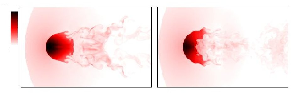
Figure 13: Density slices of the subcluster in the simulation with a $512^{3}$ static grid. Left panel: $t=2\ \mathrm{Gyr}$. Right panel: $t=3\ \mathrm{Gyr}$. The density is linearly colour coded following the colour bar on the left.

A static grid simulation of the subcluster setup has been performed with a fixed resolution of $512^{3}$ cells, corresponding to the effective resolution of the runs $A$, $D$ and $E$. The density slice at $t=2\ \mathrm{Gyr}$ (Fig. 13, left) is similar to the AMR runs, with only a higher level of symmetric structure in the wake. The symmetry is not preserved at $t=3\ \mathrm{Gyr}$ (Fig. 13, right), when the turbulent tail is very similar to the runs with new AMR criteria (Figs. 7 and 8).

Figure 14: Temporal evolution of subcluster baryonic mass fraction for the runs $A$ (solid line), the run with a $512^{3}$ static grid (dotted line) and the run $D$ as representative of the runs with new AMR criteria (dashed line). The mass fraction is normalised to its value at $t=0\ \mathrm{Gyr}$.

The evolution of the subcluster mass fraction, shown in Fig. 14, further elucidates the difference between the AMR and the static grid runs. Until $t=2\ \mathrm{Gyr}$, the static run shows a slightly larger gas stripping than run $A$, similar to run $D$, indicating a more effective description of the onset of the KHI and of the following back-flow. In the late phase and especially after $t=3\ \mathrm{Gyr}$ this trend reverses, probably because the AMR runs fail to resolve the finest details of the dispersing structures in the subcluster tail.

To sum up, the comparison with the static grid run shows that the new AMR simulations are able to correctly reproduce the main features of the subcluster evolution (see also Table 2), though the fixed grid is more effective in the very late phase of the gas stripping. The benefit of AMR can be fully appreciated also from the computational point of view: in the case of idealised subcluster simulations, the use of such a static grid causes an additional computational cost of a factor from 15 to 40, depending on the AMR criteria, with increases also for the memory requirements and the output storage.

6 Discussion and conclusions

We presented an interesting case of new refinement techniques, developed for resolving turbulent flows in AMR hydrodynamical simulations, which may have useful applications in astrophysical problems. The AMR is not only a tool used for this study, but has itself been investigated and tested in its capabilities. New refinement criteria based on the regional variability of control variables of the flow were introduced and shown to be superior for simulations of turbulent media.

As a first application, we presented a set of simulations of an idealised substructure in a wind in order to study a subcluster merger in a simplified fashion. In this setup, the novel AMR criteria are suitable for the study of the turbulent wake, which is better resolved than using refinement criteria based on local gradients of selected hydrodynamical variables. The optimal control of the refining procedure ensures high resolution where desired, as pointed out by the comparison with an equivalent static grid simulation.

The overall evolution of the subcluster is similar to the hydrodynamical simulations of Acreman et al. (2003), Takizawa (2005a) and Takizawa (2005b), where the development of shear instability leads to the formation of a turbulent wake. The typical rms velocity in the wake is of the order of $500\ \mathrm{km\ s^{-1}}$, similar to the above cited simulations and to the theoretical predictions (Subramanian et al., 2006). This value is obtained only in runs using the new AMR criteria and tends to the result from an equivalent static grid simulation, whereas in the reference run $A$ the inferred turbulent velocity is smaller by a factor of 2.

We investigated the proper refining of the turbulent wake with several numerical experiments. The choice of the AMR criteria has an impact both on the turbulent velocity and on the morphology of the subcluster core as a result of the back-flow. We claim that this issue should be carefully considered in numerical simulations of subcluster mergers, as for instance in studies of cold fronts. If the problem is addressed with an inadequate numerical setup (as in run $A$), the turbulent back-flow will be underestimated significantly. In extreme cases (run $B$, or Sect. 5.3.1), the simulation might fail to reproduce the flow downstream of the subcluster. We further showed that refining turbulence in the wake does not depend only on AMR but, as expected, also on the hydrodynamic solver. A detailed code comparison in this setup, like the one performed for the blob test by Agertz et al. (2007), would certainly be useful.

As already stated, we do not intend to discuss the features of the cold front which forms ahead of the subcluster because our simulations do not include the magnetic field evolution and/or heat conduction (Asai et al., 2004, 2005, 2007; Xiang et al., 2007). The observed cold front temperature profiles (the best studied example is A3667) call for the suppression of the thermal conduction at the interface between the cold subcluster gas and the hot ICM background (Markevitch & Vikhlinin, 2007). This suppression, in turn, would be naturally explained by a magnetic flux tangential to the cold front surface. Dursi & Pfrommer (2008) show, with MHD simulations using AMR, that the flow past a moving bullet generates vorticity, even if a magnetic field stabilises its surface against the KHI. The presence of MHD turbulence and further amplification of the magnetic field is also suggested. Despite the simplified approach of both setups, we infer that the generation of a turbulent wake and a proper modelling of this phase are therefore crucial also for the subcluster MHD simulations, and particular care in modelling the turbulent flow should be taken also in this class of simulations (with AMR or not). Only a clear assessment of the capability of a code in dealing with turbulent flows can allow to distinguish, for example, between the instability suppression caused by a magnetic field, and an unreliable modelling of the KHI onset.

Our simplified approach to the minor merger case shares the limitations of previous, similar simulations cited above. However, it has the advantage of presenting a well controlled setup, which would be difficult to study in detail in the framework of a full cosmological simulation. In view of the results it is necessary to note that, in the performed simulations, the merging subcluster was embedded in a background with a very simple velocity field. In a less idealised flow (cf. Norman & Bryan 1999; Dolag et al. 2005), it is admittedly unlikely that the turbulent tail would extend for several subcluster radii without being mixed. Nonetheless, it would not prevent from testing the turbulent character of the flow immediately downstream of the subcluster (Takizawa, 2005b), both observationally and in cosmological simulations.

From an observational point of view, the turbulence level of the subcluster wake can be an interesting test for supporting the studied scenario. The rms velocity behind the subcluster can be used as an observable for turbulence for future X-ray spectrometers. This test would pertain to the wider, long-standing problem of detecting turbulence in galaxy clusters (Schekochihin & Cowley, 2006, and reference therein, for an overview).

Although significant efforts are undertaken for modelling turbulent flows in SPH simulations (Dolag et al., 2005; Vazza et al., 2006), grid-based AMR simulations are a very powerful approach to simulations in this field. The AMR criteria used in this work will be further applied to astrophysical problems, the next step being the simulation of galaxy cluster formation and evolution (cf. Paper II). According to the analysis of Subramanian et al. (2006), besides the minor merger phase there are several other physical regimes when turbulence evolves and can play an important role in the energy budget of a galaxy cluster. The present study corroborates the importance of the minor mergers in the production of turbulence in galaxy clusters. Moreover, it provides new tools for the theoretical study of this problem, which will be continued in Paper II. The final goal of our investigation is a consistent AMR modelling of turbulent flows based on a subgrid scale model approach (cf. Schmidt et al. 2006a, b). This will be the topic of forthcoming work.

References

- Acreman et al. (2003) Acreman D. M., Stevens I. R., Ponman T. J., Sakelliou I., 2003, MNRAS, 341, 1333
- Agertz et al. (2007) Agertz O., Moore B., Stadel J., Potter D., Miniati F., Read J., Mayer L., Gawryszczak A., Kravtsov A., Nordlund A., Pearce F., Quilis V., Rudd D., Springel V., Stone J., Tasker E., Teyssier R., Wadsley J., Walder R., 2007, MNRAS, 380, 963
- Asai et al. (2004) Asai N., Fukuda N., Matsumoto R., 2004, ApJ, 606, L105
- Asai et al. (2005) —, 2005, Advances in Space Research, 36, 636
- Asai et al. (2007) —, 2007, ApJ, 663, 816
- Ascasibar & Markevitch (2006) Ascasibar Y., Markevitch M., 2006, ApJ, 650, 102
- Bialek et al. (2002) Bialek J. J., Evrard A. E., Mohr J. J., 2002, ApJ, 578, L9
- Bryan et al. (1995) Bryan G. L., Norman M. L., Stone J. M., Cen R., Ostriker J. P., 1995, Computer Physics Communications, 89, 149
- Cavaliere & Fusco-Femiano (1978) Cavaliere A., Fusco-Femiano R., 1978, A&A, 70, 677
- Churazov et al. (2004) Churazov E., Forman W., Jones C., Sunyaev R., Böhringer H., 2004, MNRAS, 347, 29
- Dolag et al. (2005) Dolag K., Vazza F., Brunetti G., Tormen G., 2005, MNRAS, 364, 753
- Drazin & Reid (2004) Drazin P. G., Reid W. H., 2004, Hydrodynamic Stability. Cambridge University Press, Cambridge
- Dursi & Pfrommer (2008) Dursi L. J., Pfrommer C., 2008, ApJ, 677, 993
- Enßlin & Vogt (2006) Enßlin T. A., Vogt C., 2006, A&A, 453, 447
- Fabian et al. (2003) Fabian A. C., Sanders J. S., Crawford C. S., Conselice C. J., Gallagher J. S., Wyse R. F. G., 2003, MNRAS, 344, L48
- Heinz et al. (2003) Heinz S., Churazov E., Forman W., Jones C., Briel U. G., 2003, MNRAS, 346, 13
- Iapichino & Niemeyer (2008) Iapichino L., Niemeyer J. C., 2008, MNRAS, accepted, arXiv Astrophysics e-prints 0801.4729 (Paper II)
- Markevitch & Vikhlinin (2007) Markevitch M., Vikhlinin A., 2007, Phys. Rep., 443, 1
- McCarthy et al. (2007) McCarthy I. G., Bower R. G., Balogh M. L., Voit G. M., Pearce F. R., Theuns T., Babul A., Lacey C. G., Frenk C. S., 2007, MNRAS, 376, 497
- Murray et al. (1993) Murray S. D., White S. D. M., Blondin J. M., Lin D. N. C., 1993, ApJ, 407, 588
- Nagai & Kravtsov (2003) Nagai D., Kravtsov A. V., 2003, ApJ, 587, 514
- Norman (2005) Norman M. L., 2005, in Plewa T., Linde T., Weirs V.G, eds, Lecture Notes in Computational Science and Engineering, Vol. 41, Adaptive Mesh Refinement – Theory and Applications. Springer, Berlin, New York, p. 413
- Norman & Bryan (1999) Norman M. L., Bryan G. L., 1999, in Lecture Notes in Physics, Berlin Springer Verlag, Vol. 530, The Radio Galaxy Messier 87, Röser H.-J., Meisenheimer K., eds., p. 106
- O’Shea et al. (2005) O’Shea B. W., Bryan G., Bordner J., Norman M. L., Abel T., Harkness R., Kritsuk A., 2005, in Plewa T., Linde T., Weirs V.G, eds, Lecture Notes in Computational Science and Engineering, Vol. 41, Adaptive Mesh Refinement – Theory and Applications. Springer, Berlin, New York, p. 341
- Paterson (1984) Paterson A. R., 1984, A First Course in Fluid Dynamics. Cambridge University Press, Cambridge
- Rebusco et al. (2005) Rebusco P., Churazov E., Böhringer H., Forman W., 2005, MNRAS, 359, 1041
- Rebusco et al. (2006) —, 2006, MNRAS, 372, 1840
- Ricker (1998) Ricker P. M., 1998, ApJ, 496, 670
- Ricker & Sarazin (2001) Ricker P. M., Sarazin C. L., 2001, ApJ, 561, 621
- Robinson et al. (2004) Robinson K., Dursi L. J., Ricker P. M., Rosner R., Calder A. C., Zingale M., Truran J. W., Linde T., Caceres A., Fryxell B., Olson K., Riley K., Siegel A., Vladimirova N., 2004, ApJ, 601, 621
- Roettiger et al. (1996) Roettiger K., Burns J. O., Loken C., 1996, ApJ, 473, 651
- Roettiger et al. (1998) Roettiger K., Stone J. M., Mushotzky R. F., 1998, ApJ, 493, 62
- Schekochihin & Cowley (2006) Schekochihin A. A., Cowley S. C., 2006, Physics of Plasmas, 13, 6501
- Schmidt et al. (2008) Schmidt W., Federrath C., Hupp M., Kern S., Niemeyer J. C., 2008, A&A, submitted
- Schmidt et al. (2006a) Schmidt W., Niemeyer J. C., Hillebrandt W., 2006a, A&A, 450, 265
- Schmidt et al. (2006b) Schmidt W., Niemeyer J. C., Hillebrandt W., Röpke F. K., 2006b, A&A, 450, 283
- Schuecker et al. (2004) Schuecker P., Finoguenov A., Miniati F., Böhringer H., Briel U. G., 2004, A&A, 426, 387
- Stone & Norman (1992a) Stone J. M., Norman M. L., 1992a, ApJS, 80, 753
- Stone & Norman (1992b) —, 1992b, ApJS, 80, 791
- Subramanian et al. (2006) Subramanian K., Shukurov A., Haugen N. E. L., 2006, MNRAS, 366, 1437
- Sunyaev et al. (2003) Sunyaev R. A., Norman M. L., Bryan G. L., 2003, Astronomy Letters, 29, 783
- Takizawa (2000) Takizawa M., 2000, ApJ, 532, 183
- Takizawa (2005a) —, 2005a, ApJ, 629, 791
- Takizawa (2005b) —, 2005b, Advances in Space Research, 36, 626
- Tittley & Henriksen (2005) Tittley E. R., Henriksen M., 2005, ApJ, 618, 227
- Vazza et al. (2006) Vazza F., Tormen G., Cassano R., Brunetti G., Dolag K., 2006, MNRAS, 369, L14
- Vietri et al. (1997) Vietri M., Ferrara A., Miniati F., 1997, ApJ, 483, 262
- Vikhlinin et al. (2001a) Vikhlinin A., Markevitch M., Murray S. S., 2001a, ApJ, 549, L47
- Vikhlinin et al. (2001b) —, 2001b, ApJ, 551, 160
- Vikhlinin & Markevitch (2002) Vikhlinin A. A., Markevitch M. L., 2002, Astronomy Letters, 28, 495
- Woodward & Colella (1984) Woodward P., Colella P., 1984, Journal of Computational Physics, 54, 115
- Xiang et al. (2007) Xiang F., Churazov E., Dolag K., Springel V., Vikhlinin A., 2007, MNRAS, 379, 1325
- Zingale et al. (2002) Zingale M., Dursi L. J., ZuHone J., Calder A. C., Fryxell B., Plewa T., Truran J. W., Caceres A., Olson K. amd Ricker P. M., Riley K., Rosner R., Siegel A., Timmes F. X., Vladimirova N., 2002, ApJS, 143, 539