Regular patterns in the acoustic spectrum of rapidly rotating stars

Abstract

Context. Rapid rotation modifies the structure of the frequency spectrum of pulsating stars, thus making mode identification difficult.

Aims. We look for new forms of organisation for the frequency spectrum that can provide a basis for mode identification at high rotation rates.

Methods. Acoustic modes in uniformly rotating polytropic models of stars are computed using a numerical code that fully takes the effects of rotation (centrifugal distortion and Coriolis acceleration) into account. All low-degree modes, $\ell=0$ to $3$, with radial orders $n=1-10$ and $21-25$ for $N=3$ polytropic models and $n=1-10$ for $N=1.5$ polytropic models are followed from a zero rotation rate up to $59\,\%$ of the break-up velocity.

Results. We find an empirical formula that gives a good description of the high-frequency range of the computed acoustic spectrum for high rotation rates. Differences between this formula and complete eigenmode calculations are shown to be substantially smaller than those obtained with a $3^{\mathrm{rd}}$ order perturbative method valid at low rotation rates.

1 Introduction

Asteroseismology has provided a way of probing stellar interiors based on the interpretation of observable stellar pulsations. In order for such interpretations to be successful, it is necessary to identify pulsation frequencies by correctly associating them with theoretically calculated pulsation modes. This is important because the geometry of a pulsation mode determines which regions of the star it probes. One way of doing this is by using regular patterns which occur in stellar frequency spectra. While being quite successful in the case of the Sun and a number of slowly rotating stars (Michel, 2006), mode identification based on pattern recognition has proved to be very difficult in rapidly rotating stars (e.g. Goupil et al., 2005). One of the basic reasons for this is that a proper understanding of the structure of the frequency spectrum has not yet been achieved in the case of such stars. Up to now, mainly perturbative methods, valid at low rotation rates, have been used to evaluate the effects of rotation on pulsation modes and their frequencies. While providing a useful context in which to interpret pulsations of slowly rotating stars, they are unable to correctly predict the structure of the frequency spectrum in rapidly rotating stars. This is particularly clear in Fig. 5 of Reese et al. (2006), in which perturbative calculations of frequencies are compared with complete eigenmode calculations for a polytropic stellar model rotating at $59\,\%$ of the critical angular velocity. As a result, many stars remain out of reach for asteroseismology. This mainly concerns early-type stars such as $\delta$ Scuti, which can reach projected equatorial velocities $(v\cdot\sin i)$ of $200\,\,\mathrm{km.s}^{-1}$ (Rodríguez et al., 2000), $\beta$ Cephei stars ($v\cdot\sin i\lesssim 300\,\,\mathrm{km.s}^{-1}$, Stankov & Handler, 2005), and $\zeta$ Oph stars ($v\cdot\sin i\lesssim 400\,\,\mathrm{km.s}^{-1}$, Balona & Dziembowski, 1999). Interestingly, the star $\zeta$ Oph ($v\cdot\sin i=380\,\,\mathrm{km.s}^{-1})$ has been observed by MOST and WIRE, thus revealing the presence of 19 different pulsation modes (Walker et al., 2005, Bruntt, private communications).

Recently, Lignières et al. (2006a) and Reese et al. (2006) came up with a numerical code which overcomes the limitations of perturbative methods and enables one to accurately evaluate the effects of rapid rotation on stellar pulsations. By analysing their results, it is possible to gain a better understanding of the structure of the frequency spectrum at rapid rotation rates. In the case of spherically symmetric stars, the origin of the regular frequency patterns can be attributed to the integrability of the ray dynamics which asymptotically describes the acoustic wave propagation (Gough, 1993). However, in the case of rapidly rotating stars, acoustic ray dynamics is no longer integrable (Lignières et al., 2006b), and it is an open question whether or not patterns will appear in the spectrum of frequencies. Nonetheless, Lignières et al. (2006a) have shown that for axisymmetric modes calculated without the Coriolis force, it is possible to obtain asymptotic patterns in the spectrum of frequencies.

In this paper, using again stellar polytropic models and a complete non-perturbative computation of their axisymmetric and non-axisymmetric acoustic modes, we show that regular frequency patterns are present in the acoustic spectrum and that they can be used to identify modes.

2 An empirical formula

In order to obtain frequency patterns for rapidly rotating stars, we start off with the set of pulsation frequencies computed in Reese et al. (2006) plus some additional frequencies. The $n=1-10,\,\,21-25$, $\ell=0-3$, $m=-\ell$ to $\ell$ modes for $N=3$ polytropic models, and the $n=1-10$, $\ell=0-3$, $m=-\ell$ to $\ell$ modes for $N=1.5$ polytropic models were followed from a zero rotation rate up to $59\,\%$ of the break-up velocity. This enabled us to label the modes in rapidly rotating stars based on their correspondence with modes in non-rotating stars. We looked for patterns in this frequency spectrum and found that the frequencies approximately obey the following empirical formula in a corotating frame:

$$\omega_{n,\,\ell,\,m}=\Delta_{n}n+\Delta_{\ell}\ell+\Delta_{m}|m|+\alpha^{\pm}$$ (1)

In order to obtain frequencies in an inertial frame, one needs to add the geometrical term $-m\Omega$.

This formula is a generalisation of Eq. (42) of Lignières et al. (2006a) by including the Coriolis effect and the case of non-axisymmetric modes. The terms $\Delta_{n}$, $\Delta_{\ell}$, $\Delta_{m}$ and $\alpha^{\pm}$, which depend on the stellar structure, have been computed here for different rotation rates. The parameter $\alpha^{+}$ (resp. $\alpha^{-}$) is an additive constant for symmetric, $\ell+m$ even (resp. antisymmetric, $\ell+m$ odd), modes with respect to the equator. We note that the term for non-axisymmetric modes depends on $|m|$ rather than $m$. Indeed, at rapid rotation rates or high radial orders, the effects of the Coriolis force become negligible in comparison with the effects of the centrifugal force, as can be seen in Fig. 6 of Reese et al. (2006). The centrifugal force leads to frequency shifts which do not depend on the sign of $m$. In order to know how these shifts scale with $|m|$, we plot in Fig. 1 the differences $\left(\omega_{n,\,\ell,\,m}-\omega_{n,\,\ell,\,m-2.\mathrm{sg}(m)}\right)/2$ as a function of the radial order. We increment the azimuthal order by $2$ rather than $1$ to insure that the two modes have the same parity. As shown in Fig. 1, these differences converge towards a limit which slightly depends on $|m|$ as the radial order increases. This justifies using a linear dependence on $|m|$ as a first approximation. The fact that these increments only converge at high radial orders shows that Eq. (1) describes an asymptotic behaviour of the computed acoustic modes.

Figure 1: Frequency differences $\Delta_{m}=\frac{\omega_{n,\ell,\,m}-\omega_{n,\ell,\,m-2\cdot\mathrm{sg}(m)}}{2}$ as a function of the radial order $n$ for the $N=3$ polytropic models. The frequencies have been scaled by $\Omega_{\star}$. For high radial orders, these differences converge to a limit which does not depend on $\ell$ or $m$.

In Table 1, we give the values of $\Delta_{n}$, $\Delta_{\ell}$, $\Delta_{m}$, $\alpha^{+}$ and $\alpha^{-}$, scaled by $\Omega_{\star}$, for $N=3$ polytropic models. These are given for different rotation rates scaled either by $\Omega_{\star}=\sqrt{GM/R_{\mathrm{pol}}^{3}}$ or by $\Omega_{\mathrm{K}}=\sqrt{GM/R_{\mathrm{eq}}^{3}}$, the Keplerian break-up velocity, where $R_{\mathrm{eq}}$ (resp. $R_{\mathrm{pol}}$) is the equatorial (resp. polar) radius. These values were obtained by calculating various frequency separations and averaging them for radial orders $21\leq n\leq 25$. At zero rotation, they agree pretty well with the theoretical values, $\Delta_{n}/\Omega_{\star}=1.238$ and $\Delta_{\ell}/\Omega_{\star}=0.619$ corresponding to the asymptotic description of low degree and high order acoustic modes in non-rotating stars (Mullan & Ulrich, 1988). The last line contains the same parameters but calculated for frequencies in which the Coriolis force has been neglected. The fact that it is essentially the same as the line before shows that the Coriolis force plays almost no role in Eq. (1) nor ultimately in the frequency spectrum for sufficiently high radial orders.

$\frac{\Omega}{\Omega_{\mathrm{K}}}$	$\frac{\Omega}{\Omega_{\star}}$	$\frac{\Delta_{n}}{\Omega_{\star}}$	$\frac{\Delta_{\ell}}{\Omega_{\star}}$	$\frac{\Delta_{m}}{\Omega_{\star}}$	$\frac{\alpha^{+}}{\Omega_{\star}}$	$\frac{\alpha^{-}}{\Omega_{\star}}$
0.000	0.000	1.248	0.543	0.000	1.758	1.761
0.037	0.037	1.246	0.545	-0.007	1.757	1.764
0.111	0.110	1.239	0.515	-0.031	1.770	1.843
0.186	0.181	1.234	0.395	-0.031	1.727	1.942
0.262	0.249	1.229	0.279	-0.036	1.680	2.006
0.339	0.311	1.220	0.191	-0.064	1.614	2.020
0.419	0.368	1.194	0.189	-0.142	1.666	2.068
0.502	0.419	1.154	0.201	-0.182	1.661	2.036
0.589	0.461	1.102	0.194	-0.185	1.598	1.953
0.589	0.461	1.102	0.194	-0.185	1.587	1.943

Table 1: Coefficients for Eq. (1), for $N=3$ polytropes.

An important consequence of the values given in Table 1 concerns the small frequency separation. In non-rotating stars, the so-called small frequency separation $\omega_{n+1,\ell,m}-\omega_{n,\ell+2,m}$ goes to zero in the high frequency limit because the ratio $\Delta_{n}/\Delta_{\ell}$ is $2$. For rapidly rotating stars, Table 1 clearly shows that this ratio departs from $2$ by taking on larger values. This, of course, invalidates the use of the small frequency separation as a mode identification scheme.

In Fig. 2, we plot $\Delta_{n}$ scaled with different quantities as a function of $\Omega$. As can be seen from the figure, $\Delta_{n}$ is roughly proportional to $\sqrt{GM/V}$ where $M$ is the mass and $V$ the volume of the star. This suggests that $\Delta_{n}$ may be related in a simple way to the mean density of the star.

Figure 2: The large frequency separation $\Delta_{n}$ as a function of the rotation rate $\Omega$. $\Delta_{n}$ has been scaled with different quantities so as to show which other stellar quantity best matches this frequency separation. As can be seen, $\Delta_{n}$ is roughly proportional to the square root of the mean density of the star.

3 Accuracy of the formula

We now turn our attention to evaluating the accuracy of the formula (1). In Fig. 3, we plot the correspondence between a spectrum based on Eq. (1) and the frequencies given by the eigenmode calculations for $\Omega=0.59\,\Omega_{K}$. As can be seen, the two sets of frequencies match pretty well, especially for high radial orders. This represents a drastic improvement over $3^{\mathrm{rd}}$ order perturbative calculations (see Fig. 5 of Reese et al. 2006).

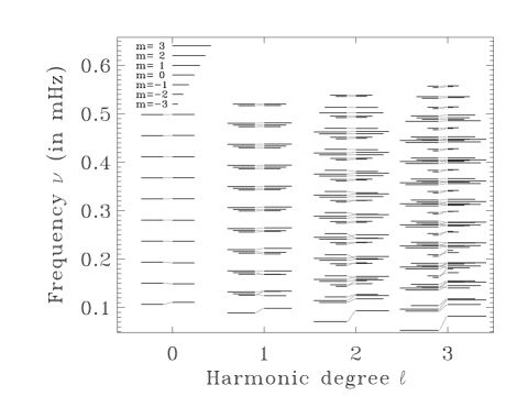
Figure 3: Comparison between frequencies based on Eq. (1) and complete eigenmode calculations, both of which are given in an inertial frame. $\ell$ and $m$ are indicated on the figure, and the radial orders are $n=1$ to $10$. This figure contains four columns subdivided into two, the left part corresponding to Eq. (1) and the right part to complete calculations. The oblique grey lines in between show the correspondence between the two sets of frequencies. The units are the same as in Fig. 5 of Reese et al. (2006), which allows direct comparison. As can be seen from comparing these figures, Eq. (1) gives a much better description of the frequency spectrum than a $3^{\mathrm{rd}}$ order perturbative formula.

Table 2 contains the mean quadratic error $\left<\mathcal{E}\right>^{1/2}$ both for $3^{\mathrm{rd}}$ order perturbative calculations and empirical ones. These errors as well as the probability $p$ of mode inversion (explained below) have been calculated for modes with ${21\leq n\leq 25}$ except for the last line where $1\leq n\leq 10$. Physically, an error of $0.0036\,\Delta_{n}$ at $\Omega=0.59\,\Omega_{K}$ corresponds to $0.16\,\,\mathrm{\mu Hz}$ for an $M=1.9\,M_{\odot}$, $R_{\mathrm{pol}}=2.3R_{\odot}$, $N=3$ polytropic star. The errors on the last line can be made smaller by calculating the increments $\Delta_{n}$, $\Delta_{\ell}$ etc. using radial orders $1\leq n\leq 10$, which in practise observers are likely to do.

Another useful quantity to appreciate the reliability of an approximate formula at mode identification is the probability $p$ of inverting the identification of two randomly selected frequencies when using such a formula. This probability is defined as:

$$p=\frac{\mbox{Number of inversions}}{\mbox{Number of pairs of modes}}$$ (2)

where an inversion occurs for modes $A$ and $B$ when $\left(\omega_{A}^{\mathrm{approx.}}-\omega_{B}^{\mathrm{approx.}}\right)\left(\omega_{A}-\omega_{B}\right)<0$. $p=1$ corresponds to a spectrum in reverse order, whereas $p=0$ means the order is identical. In Table 2, $p$ is calculated for both methods, based on frequencies in the inertial frame so as to be closer to observations. For example, $p=0.0035$ means that out of $3160$ frequency pairs, $11$ were inverted. As shown, the empirical formula gives a far better idea of the order in which modes appear in the frequency spectrum at $\Omega=0.59\,\Omega_{K}$ than a $3^{\mathrm{rd}}$ order perturbative approach.

	Perturbative		Asymptotic
$\frac{\Omega}{\Omega_{\mathrm{K}}}$	$\frac{\left<\mathcal{E}^{2}\right>^{1/2}}{\Delta_{n}}$	$p$	$\frac{\left<\mathcal{E}^{2}\right>^{1/2}}{\Delta_{n}}$	$p$
0.037	0.0005	0.0000	0.0114	0.0000
0.111	0.0370	0.0054	0.0141	0.0044
0.186	0.1793	0.0294	0.0124	0.0022
0.262	0.4325	0.0595	0.0135	0.0047
0.339	0.7436	0.0826	0.0174	0.0041
0.419	0.9924	0.1073	0.0109	0.0013
0.502	1.0674	0.1237	0.0085	0.0025
0.589	0.9885	0.1497	0.0036	0.0035
0.589	0.3506	0.0319	0.1235	0.0059

Table 2: Different measurements of the errors for the perturbative and empirical methods (for $N=3$).

As expected, the perturbative method gives best results for low rotation rates, while Eq. (1) is more efficient above $\Omega=0.11\,\Omega_{\mathrm{K}}$, for high radial orders. This is because, by construction, Eq. (1) preserves the regularity of the frequency spectrum whereas perturbative methods do not. Also, comparing the last two lines of Table 2 again shows that Eq. (1) works better for high frequencies, whereas the perturbative approach works better for low frequencies, where the centrifugal force has a smaller effect.

4 Discussion

The preceding sections show that at rapid rotation rates, it is possible to describe the computed frequency spectrum using a formula similar to the asymptotic one found by Tassoul (1980). Quite significantly, table 2 shows that the accuracy of this formula increases at high rotations, thus suggesting that eigenmodes reach an asymptotic régime at lower radial orders for these rapid rotations.

In the rapid rotation régime, a forthcoming study based on ray dynamics (Lignières & Georgeot, 2008) shows that Eq. (1) holds for low-degree, high order modes which concentrate at middle latitudes as rotation increases. This modification of mode geometry leads to a reorganisation of node placement as can be seen in Fig. 3 of Reese (2008), characterised by a different set of quantum numbers, $(\tilde{n}=2n+\varepsilon,\tilde{\ell}=\frac{\ell-|m|-\varepsilon}{2},\tilde{m}=m)$ where $\varepsilon=(l+m)\,\,\mod\,\,2$. Based on these quantum numbers, Eq. (1) then takes on the following form:

$$\omega_{n,\,\ell,\,m}=\tilde{\Delta}_{n}\tilde{n}+\tilde{\Delta}_{\ell}\tilde{\ell}+\tilde{\Delta}_{m}|m|+\tilde{\alpha}^{\pm}$$ (3)

where $\tilde{\Delta}_{n}=\Delta_{n}/2$, $\tilde{\Delta}_{\ell}=2\Delta_{\ell}$, $\tilde{\Delta}_{m}=\Delta_{\ell}+\Delta_{m}$, $\tilde{\alpha}^{+}=\alpha^{+}$ and $\tilde{\alpha}^{-}=\alpha^{-}+\Delta_{\ell}-\Delta_{n}/2$. With the numerical values from Table 1, we find that $\tilde{\alpha}^{+}\simeq\tilde{\alpha}^{-}$. The same also applies for the $N=1.5$ polytropic model. This suggests that the true asymptotic formula is closer to Eq. (3) in which $\tilde{\alpha}^{+}=\tilde{\alpha}^{-}=\tilde{\alpha}$. Applying this new formula leads to errors which are only slightly larger in spite of the fact there is now one less free parameter.

Equation (3) also accentuates the $|m|$ dependence of the azimuthal term since $\tilde{\Delta}_{m}$ is of the same order of magnitude as the variation on $\Delta_{m}$. This suggests that the azimuthal term $\tilde{\Delta}_{m}$ expressed in these new quantum numbers should take on a different form, and calls for further investigation. But as can be seen from Table 2, Eqs. (1) and (3) remain effective at identifying low-degree (observable) pulsation modes.

For higher degree modes, Lignières et al. (2006b) pointed out the existence of other types of modes, namely chaotic and whispering gallery modes, which correspond, respectively, to intermediate and high values of $\ell$ at zero rotation. As shown in Lignières & Georgeot (2008), the frequency spectra of these modes have different organisations.

Finally, it must be underlined that the results presented here are based on polytropic stellar models. Naturally, the question arises whether or not these patterns still exist in the case of more realistic models. In the non-rotating case, sharp chemical gradients lead to the break-down of the assumptions behind asymptotic analysis. Nonetheless, rather than removing the equidistant frequency pattern, these lead to a periodic component which is added to the asymptotic formula (e.g. Gough, 1990). If the rapidly rotating case behaves similarly, then it may be expected that these sharp chemical gradients also merely perturb the asymptotic frequency pattern without removing it altogether.

5 Conclusion

The formulae (1) and (3) that we presented are the signature of an asymptotic régime of high order acoustic oscillations in rapidly rotating polytropic stars. As opposed to perturbative methods, which are valid at low rotation rates, they give an accurate description of the frequency spectrum by preserving its basic structure and consequently provide a basis for mode identification schemes. This is a timely result as seismology space missions are collecting large data sets of unprecedented quality on rapidly rotating stars.

A key issue for future theoretical studies will be to relate the seismic observables $\tilde{\Delta}_{n},\tilde{\Delta}_{\ell}$ and $\tilde{\Delta}_{m}$ to the physical properties of the star. Acoustic ray dynamics combined with semi-classical quantization methods is expected to play a crucial role in this context.