Recursive Bias Estimation and Boosting
Abstract
This paper presents a general iterative bias correction procedure for regression smoothers. This bias reduction schema is shown to correspond operationally to the Boosting algorithm and provides a new statistical interpretation for Boosting. We analyze the behavior of the Boosting algorithm applied to common smoothers which we show depend on the spectrum of . We present examples of common smoother for which Boosting generates a divergent sequence. The statistical interpretation suggest combining algorithm with an appropriate stopping rule for the iterative procedure. Finally we illustrate the practical finite sample performances of the iterative smoother via a simulation study. simulations.
keywords:
[class=AMS]keywords:
, and
1 Introduction
Regression is a fundamental data analysis tool for uncovering functional relationships between pairs of observations . The traditional approach specifies a parametric family of regression functions to describe the conditional expectation of the dependent variable given the independent variables , and estimates the free parameters by minimizing the squared error between the predicted values and the data. An alternative approach is to assume that the regression function varies smoothly in the independent variable and estimate locally the conditional expectation of given . This results in nonparametric regression estimators (e.g. Fan and Gijbels (1996); Hastie and Tibshirani (1995); Simonoff (1996)). The vector of predicted values at the observed covariates from a nonparametric regression is called a regression smoother, or simply a smoother, because the predicted values are less variable than the original observations .
Over the past thirty years, numerous smoothers have been proposed: running-mean smoother, running-line smoother, bin smoother, kernel based smoother (Nadaraya (1964); Watson (1964)), spline regression smoother, smoothing splines smoother (Whittaker (1923); Wahba (1990)), locally weighted running-line smoother (Cleveland (1979)), just to mention a few. We refer to Buja et al. (1989); Eubank (1988); Fan and Gijbels (1996); Hastie and Tibshirani (1995) for more in depth treatments of regression smoothers.
An important property of smoothers is that they do not require a rigid (parametric) specification of the regression function. That is, we model the pairs as
| (1.1) |
where is an unknown smooth function. The disturbances are independent mean zero and variance random variables that are independent of the covariates , . To help our discussion on smoothers, we rewrite Equation (1.1) compactly in vector form by setting , and , to get
| (1.2) |
Finally we write , the vector of fitted values from the regression smoother at the observations. Operationally, linear smoothers can be written as
where is a smoothing matrix. While in general the smoothing matrix will be not be a projection, it is usually a contraction (Buja et al. (1989)). That is, .
Smoothing matrices typically depend on a tuning parameter, which denoted by , that governs the tradeoff between the smoothness of the estimate and the goodness-of-fit of the smoother to the data. We parameterize the smoothing matrix such that large values of will produce very smooth curves while small will produce a more wiggly curve that wants to interpolate the data. The parameter is the bandwidth for kernel smoother, the span size for running-mean smoother, bin smoother, and the penalty factor for spline smoother.
Much has been written on how to select an appropriate smoothing parameter, see for example (Simonoff (1996)). Ideally, we want to choose the smoothing parameter to minimize the expected squared prediction error. But without explicit knowledge of the underlying regression function, the prediction error can not be computed. Instead, one minimizes estimates of the prediction error using Stein Unbiased Risk Estimate or Cross-Validation (Li (1985)).
This paper takes a different approach. Instead of selecting the tuning parameter , we fix it to some reasonably large value, in a way that ensures that the resulting smoothers oversmooths the data, that is, the resulting smoother will have a relatively small variance but a substantial bias. Observe that the conditional expectation of the given is the bias of the smoother. This provides us with the opportunity of estimating the bias by smoothing the residuals , thereby enabling us to bias correct the initial smoother by subtracting from it the estimated bias. The idea of estimating the bias from residuals to correct a pilot estimator of a regression function goes back to the concept of twicing introduced by (Tukey (1977)) to estimate bias from model misspecification in multivariate regression. Obviously, one can iteratively repeat the bias correction step until the increase to the variance from the bias correction outweighs the magnitude of the reduction in bias, leading to an iterative bias correction.
Another iterative function estimation method, seemingly unrelated to bias reduction, is Boosting. Boosting was introduced as a machine learning algorithm for combining multiple weak learners by averaging their weighted predictions (Schapire (1990); Freund (1995)). The good performance of the Boosting algorithm on a variety of datasets stimulated statisticians to understand it from a statistical point of view. In his seminal paper, Breiman (1998) shows how Boosting can be interpreted as a gradient descent method. This view of Boosting was reinforced by Friedman (2001). Adaboost, a popular variant of the Boosting algorithm, can be understood as a method for fitting an additive model (Friedman et al. (2000)) and recently Efron et al. (2004) made a connection between Boosting and Lasso for linear models.
But connections between iterative bias reduction and Boosting can be made. In the context of nonparametric density estimation, Di Marzio and Taylor (2004) have shown that one iteration of the Boosting algorithm reduced the bias of the initial estimator in a manner similar to the multiplicative bias reduction methods (Hjort and Glad (1995); Jones et al. (1995); Hengartner and Matzner-Løber (2007)). In the follow-up paper (Di Marzio and Taylor (2007)), they extend their results to the nonparametric regression setting and show that one step of the Boosting algorithm applied to an oversmooth effects a bias reduction. As expected, the decrease in the bias comes at the cost of an increase in the variance of the corrected smoother.
In Section 2, we show that in the context of regression, such iterative bias reduction schemes obtained by correcting an estimator by smoothers of the residuals correspond operationally to the Boosting algorithm. This provides a novel statistical interpretation of Boosting. This new interpretation helps explain why, as the number of iteration increases, the estimator eventually deteriorates. Indeed, by iteratively reducing the bias, one eventually adds more variability than one reduces the bias.
In Section 3, we discuss the behavior of the Boosting of many commonly used smoothers: smoothing splines, Nadaraya-Watson kernel and -nearest neighbor smoothers. Unlike the good behavior of the boosted smoothing splines discussed in Buhlmann and Yu (2003), we show that Boosting -nearest neighbor smoothers and kernel smoothers that are not positive definite produces a sequence of smoothers that behave erratically after a small number of iteration, and eventually diverge. The reason for the failure of the Boosting algorithm, when applied to these smoothers, is that the bias is overestimated. As a result, the Boosting algorithm over-corrects the bias and produces a divergent smoother sequence. Section 4 discusses modifications to the original smoother to ensure good behavior of the sequence of boosted smoothers.
To control both the over-fitting and over-correction problems, one needs to stop the Boosting algorithm in a timely manner. Our interpretation of the Boosting as an iterative bias correction scheme leads us to propose in Section 5 several data driven stopping rules: Akaike Information Criteria (AIC), a modified AIC, Generalized Cross Validation (GCV), one and -fold Cross Validation, and estimated prediction error estimation using data splitting. Using either the asymptotic results of Li (1987) or the finite sample oracle inequality of Hengartner et al. (2002), we see that stopped boosted smoother has desirable statistical properties. We use either of these theorems to conclude that the desirable properties of the boosted smoother does not depend on the initial pilot smoother, provided that the pilot oversmooths the data. This conclusion is reaffirmed from the simulation study we present in Section 6. To implement these data driven stopping rules, we need to calculate predictions of the smoother for any desired value of the covariates, and not only at the observations. We show in Section 5 how to extend linear smoothers to give predictions at any desired point.
The simulations in Section 6 show that when we combine a GCV based stopping rule to the Boosting algorithm seems to work well. It stops early when the Boosting algorithm misbehaves, and otherwise takes advantage of the bias reduction. Our simulation compares optimum smoothers and optimum iterative bias corrected smoothers (using generalized cross validation) for general smoothers without knowledge of the underlying regression function. We conclude that the optimal iterative bias corrected smoother outperforms the optimal smoother.
Finally, the proofs are gathered in the Appendix.
2 Recursive bias estimation
In this section, we define a class of iteratively bias corrected linear smoothers and highlight some of their properties.
2.1 Bias Corrected Linear Smoothers
For ease of exposition, we shall consider the univariate nonparametric regression model in vector form (1.2) from Section 1
where the errors are independent, have mean zero and constant variance , and are independent of the covariates , . Extensions to multivariate smoothers are strait forward and we refer to Buja et al. (1989) for example.
Linear smoothers can be written as
| (2.1) |
where is an smoothing matrix. Typical smoothing matrices are contractions, so that , and as a result the associated smoother is called a shrinkage smoother (see for example Buja et al. (1989)). Let be the identity matrix.
A natural question is “how can one estimate the bias?” To answer this question, observe that the residuals have expected value . This suggests estimating the bias by smoothing the negative residuals
| (2.3) |
This bias estimator is zero whenever the smoothing matrix is a projection, as is the case for linear regression, bin smoothers and regression splines. However, since most common smoothers are not projections, we have an opportunity to extract further signal from the residual and possibly improve upon the initial estimator.
Note that a smoothing matrix other than can be used to estimate the bias in (2.3), but as we shall see, in many examples, using works very well, and leads to an attractive interpretation of Equation (2.3). Indeed, since the matrices and commute, we can express the estimated bias as
We recognize the latter as the right-hand side of (2.2) with the smoother replacing the unknown vector . This says that is a plug-in estimate for the bias .
Subtracting the estimated bias from the initial smoother produces the twicing estimator
Since the twiced smoother is also a linear smoother, one can repeat the above discussion with replacing , producing a thriced linear smoother. We can iterate the bias correction step to recursively define a family of bias corrected smoothers. Starting with , construct recursively for , the sequences of residuals, estimated bias and bias corrected smoothers
| (2.4) |
We show in the next theorem that the iteratively bias corrected smoother defined by Equation 2.4 has a nice representation in terms of the original smoothing matrix .
Theorem 2.1.
The iterated bias corrected linear smoother (2.4) can be explicitly written as
| (2.5) | |||||
Example with a Gaussian kernel smoother Throughout the next two sections, we shall use the following example to illustrate the behavior of the Boosting algorithms applied to various common smoothers. Take the design points to be 50 independently drawn points from an uniform distribution on the unit interval . The true regression function is , the solid line in the Figure 1, and the disturbances are mean zero Gaussians with variance producing a signal to noise ratio of five.
In the next figure, the initial smoother is a kernel one, with a bandwidth equals to 0.2 and a Gaussian kernel. This pilot smoother heavily oversmooths the data, see Figure 1 that shows that the pilot smoother (plain line) is nearly constant. The iterative bias corrected estimators are plotted in figure (1) for values of , the number of iterations, in
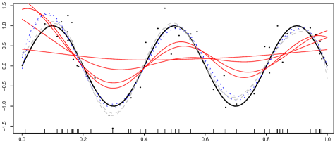
Figure 1 shows how each bias correction iteration changes the smoother, starting from a nearly constant smoother and slowly deforming (going down into the valleys and up into the peaks) with increasing number of iterations , and . After 500 iterations, the iterative smoother is very close to the true function. However when the number of iterations is very large (here and ) the iterative smoother deteriorates.
Lemma 2.2.
The squared bias and variance of the iterated bias corrected linear smoother (2.4) are
Remark: Symmetric smoothing matrices can be decomposed as , with orthonormal matrix and diagonal matrix .
| (2.6) |
Applying Lemma 2.2, we get
Hence if the magnitude of the eigenvalues of are bounded by one, each iteration of the bias correction will decrease the bias and increase the variance. This monotonicity (decreasing bias, increasing variance) with increasing number of iterations allows us consider data driven selection for number of bias correction steps to achieves the best compromise between bias and variance of the smoother.
The preceding remark suggests that the behavior of the iterative bias corrected smoother is tied to the spectrum of , and not of . The next theorem collects the various convergence results for iterated bias corrected linear smoothers.
Theorem 2.3.
Suppose that the singular values of satisfy
| (2.7) |
Then we have that
Conversely, if has a singular value , then
Remark 1: This theorem shows that iterating the booting algorithm to reach the limit of the sequence of boosted smoothers, , is not the desirable. However, since each iteration decreases the bias and increases the variance, a suitably stopped Boosting estimator is likely to improve upon the initial smoother.
Remark 2: When , the iterative bias correction fails. The reason is that overestimates the true bias , and hence Boosting repeatedly overcorrects the bias of the smoothers, which results in a divergent sequence of smoothers. Divergence of the sequence of boosted smoothers can be detected numerically, making it possible to avoid this bad behavior by combining the iterative bias correction procedure with a suitable stopping rule.
Remark 3: The assumption that for all , the singular values implies that is a contraction, so that . This condition does not imply that the smoother itself is a shrinkage smoother as defined by (Buja et al. (1989)). Conversely, not all shrinkage estimators satisfy the condition 2.7 of the theorem. In Section 3, we will given examples of common shrinkage smoothers for which , and show numerically that for these shrinkage smoothers, the iterative bias correction scheme will fail.
2.2 Boosting for regression
Boosting is one of the most successful and practical methods that arose 15 years ago from the machine learning community (Schapire (1990); Freund (1995)). In light of Friedman (2001), the Boosting algorithms has been interpreted as functional gradient descent technique. Let us summarize the Boost algorithm described in Buhlmann and Yu (2003).
Step 0: Set . Given the data , calculate an pilot regression smoother
by least squares fitting of the parameter, that is,
Step 1: With a current smoother , compute the residuals and fit the real-valued learner to the current residuals by least square. The fit is denoted by . Update
| (2.8) |
Step 2: Increase iteration index by one and repeat step 1.
Lemma 2.4 (Buhlmann and Yu, 2003).
The smoothing matrix associated with the Boosting iterate of linear smoother with smoothing matrix is
Viewing Boosting as a greedy gradient descent method, the update formula (2.8) is often modified to include convergence factor , as in Friedman (2001), to become
where is the best step toward the best direction .
This general formulation allows a great deal of flexibility, both in selecting the type of smoother used in each iteration of the Boosting algorithm, and in the selection of the convergence factor. For example, we may start with a running mean pilot smoother, and use a smoothing spline to estimate the bias in the first Boosting iteration and a nearest neighbor smoother to estimate the bias in the second iteration. However in practice, one typically uses the same smoother for all iterations and fix the convergence factor . That is, the sequence of smoothers resulting from the Boosting algorithm is given by
| (2.9) |
We shall discuss in detail in Section 4 the impact of this convergence factor and other modifications to the Boosting algorithm to ensure good behavior of the sequence of boosted smoothers.
3 Boosting classical smoothers
This section is devoted to understanding the behavior of the iterative Boosting schema using classical smoothers, which in light of Theorem 2.3, depends on the magnitude of the singular values of the matrix .
We start our discussion by noting that Boosting a projection type smoothers is of no interest because residuals are orthogonal to smoother . It follows that the smoothed residuals , and as a result, for all . Hence Boosting a bin smoother or a regression spline smoother leaves the initial smoother unchanged.
Consider the -nearest neighbor smoother. Its associated smoothing matrix is if belongs to the -nearest neighbor of and otherwise. Note that this smoothing matrix is not symmetric. While this smoother enjoys many desirable properties, it is not well suited for Boosting because the matrix has singular values larger than one.
Theorem 3.1.
In the fixed design or in the uniform design, as soon as the number of is bigger than one and smaller than , at least one singular value of is bigger than 1.
The proof of the theorem is found in the appendix. A consequence of Proposition 3.1 and Theorem 2.3, is that the Boosting algorithm applied to a -nearest neighbor smoother produces a sequence of divergent smoothers, and hence should not be used in practice.
Example continued with -nearest neighbor smoother. We confirm this behavior numerically. Using the same data as before, we apply the Boosting algorithm starting with an pilot -nearest neighbor smoother with . The pilot estimator is plotted in a plain line, and the various boosted smoothers with , the number of iterations, valued in in dotted lines.
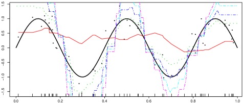
For , the pilot smoother is nearly constant (since we take neighbors) and very quickly the iterative bias corrected estimator explodes. Qualitatively, the smoothers are getting higher at the peaks and lower in the valleys, which is consistent with an overcorrection of the bias. Contrast this behavior with the one shown in Figure 1.
Kernel type smoother. For Nadaraya kernel type estimator, the smoothing matrix has entries , where is a symmetric function (e.g., uniform, Epanechnikov, Gaussian), denotes the bandwidth and is the scaled kernel . The matrix is not symmetric but can be written as where is symmetric with general element and is diagonal with element . Algebraic manipulations allows us to rewrite the iterated estimator as
Since the matrix is symmetric, we apply the classical decomposition , with orthonormal and diagonal, to get a closed form expression for the boosted smoother
The eigen decomposition of can be used to describe the behavior of the sequence of iterative estimators. In particular, any eigenvalue of that is negative or greater than 2 will lead to unstable procedure. If the kernel is a symmetric probability density function positive definite, then the spectrum of the Nadaraya-Watson kernel smoother lies between zero and one.
Theorem 3.2.
If the inverse Fourier-Stieltjes transform of a kernel is a real positive finite measure, then the spectrum of the Nadaraya-Watson kernel smoother lies between zero and one.
Conversely, suppose that are an independent -sample from a density (with respect to Lebesgue measure) that is bounded away from zero on a compact set strictly included in the support of . If the inverse Fourier-Stieltjes transform of a kernel is not a positive finite measure, then with probability approaching one as the sample size grows to infinity, the maximum of the spectrum of is larger than one.
Remark 1: Since the is the same as the and is row stochastic, we conclude that . So we are only concern by the presence of negative eigenvalues in the spectrum of .
Remark 2: In Di Marzio and Taylor (2008) proved the first part of the theorem. Our proof of the converse shows that for large enough sample sizes, most configurations from a random design lead to smoothing matrix with negative singular values.
Remark 3: The assumption that the inverse Fourier-Stieltjes transform of a kernel is a real positive finite measure is equivalent to the kernel being positive a definite function, that is, for any finite set of points , the matrix
is positive definite. We refer to Schwartz (1993) for a detailed study of positive definite functions.
The Gaussian and triangular kernels are positive definite kernels (they are the Fourier transform of a finite positive measure (Feller (1966))) and in light of Theorem 3.2 the Boosting of Nadaraya-Watson kernel smoothers with these kernels produces a sequence of well behavior smoother. However, the uniform and the Epanechnikov kernels are not positive definite. Theorem 3.2 states that for large samples, the spectrum of is larger than one and as a result the sequence of boosted smoother diverges. Proposition 3.3 below strengthen this result by stating that the largest singular value of is always larger than one.
Proposition 3.3.
Let be the smoothing matrix of a Nadaraya-Watson regression smoother based on either the uniform or the Epanechnikov kernel. Then the largest singular value of is larger than one.
Example continued with Epanechnikov kernel smoother. In the next figure, the pilot smoother is a kernel one with an Epanechnikov kernel and with bandwidth is equal to 0.15. The pilot smoother is the plain line, and the subsequent iterations with , the number of iterations, valued in , are the dotted lines.

For , the pilot smoother oversmooths the true regression since the bandwidth takes almost one third of the data and very quickly the iterative estimator explodes. Contrast this behavior with the one shown by the Gaussian kernel smoother in Figure 1.
Finally, let us now consider the smoothing splines smoother. The smoothing matrix is symmetric, and therefore admits an eigen decomposition. Denote by an orthonormal basis of eigenvectors of associated to the eigenvalues (Utreras (1983)). Denote by the orthonormal matrix of column eigenvectors and write , that is . The iterated bias reduction estimator is given by (2.6). Since all the eigenvalues are between 0 and 1, then if is large, the iterative procedure kills the eigenvalues less than 1 and put the others to 1.
Example continued with smoothing splines smoother In the next figure, the pilot smoother is a smoothing spline, with equals to 0.2. The different estimators are plotted in figure (4), with the pilot estimator in plain line and the boosted smoothers with number of iterations being in dotted lines.
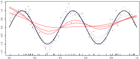
The pilot estimator is more variable than the pilot estimator of figure 1 and by the way the convergence and the deterioration arise faster.
4 Smoother engineering
Practical implementations of the Boosting algorithm include a user selected convergence factor that appears in the definition of the boosted smoother
| (4.1) |
In this section, we show that when , one effectively operates a partial bias correction. This partial bias correction does not however resolve the problems associated with Boosting a nearest neighbor or Nadaraya Watson kernel smoothers with compact kernel we exhibited in the previous section. To resolve these problems, we propose to suitably modify the boosted smoother. We call such targeted changes smoother engineering.
The following iterative partial bias reduction scheme is equivalent to the Boosting algorithm defined by Equation (4.1): Given a smoother at the iteration of the Boosting algorithm, calculate the residuals and estimated bias
Next, given , consider the partially bias corrected smoother
| (4.2) |
Algebraic manipulations of the smoothing matrix of the right-hand side of (4.2) yields
from which we conclude that satisfies (4.1) and therefore is the iteration of the Boosting algorithm. It is interesting to rewrite (4.2) as
which shows that boosted smoother is a convex combination between the smoother at iteration , and the fully bias corrected smoother . As a result, we understand how the introduction of a convergence factor produces a ”weaker learner” than the one obtained for .
In analogy to Theorem 2.3, the behavior of the sequence of the smoother depends on the spectrum of . Specifically, if , then ,and conversely, if , . Inspection of the proofs of propositions 3.1 and 3.2 reveal that the spectrum of for both the nearest neighbor smoother and the Nadaraya Watson kernel smoother has singular values of magnitude larger than one. Hence the introduction of the convergence factor does not help resolve the difficulties arising when Boosting these smoothers.
To resolve the potential convergence issues, one needs to suitably modify the underlying smoother to ensure that the magnitude of the singular values of are bounded by one. A practical solution is to replace the smoothing matrix by . If is a contraction, it follows that the eigenvalues of are nonnegative and bounded by one. Hence the Boosting algorithm with this smoother will produce a well behaved sequence of smoothers with .
While substituting the smoother for can produces better boosted smoothers in cases where Boosting failed, our numerical experimentations has shown that the performance of Boosting is not as good as Boosting when the pilot estimator enjoyed good properties, as is the case for smoothing splines and the Nadaraya Watson kernel smoother with Gaussian kernel.
5 Stopping rules
Theorem 2.3 in Section 2 states that the limit of the sequence of boosted smoothers is either the raw data or has norm . It follows that iterating the Boosting algorithm until convergence is not desirable. However, since each iteration of the Boosting algorithm reduces the bias and increases the variance, often a few iteration of the Boosting algorithm will produce a better smoother than the pilot smoother. This brings up the important question of how to decide when to stop the iterative bias correction process.
Viewing the latter question as a model selection problem suggests stopping rules based on Mallows’ (Mallows (1973)), Akaike Information Criterion, AIC, (Akaike (1973)), Bayesian Information Criterion, BIC, (Schwarz (1978)), and Generalized cross validation (Craven and Wahba (1979)). Each of these selectors estimate the optimum number of iterations of the Boosting algorithm by minimizing estimates of the expected squared prediction error of the smoothers over some pre-specified set .
Three of the six criteria we study numerically in Section 6 use plug-in estimates for the squared bias and variance of the expected prediction mean square error. Specifically, consider
| (5.1) | |||||
| (5.2) | |||||
| (5.3) |
In nonparametric smoothing, the AIC criteria (5.1) has a noticeable tendency to select more iterations than needed, leading to a final smoother that typically undersmooths the data. As a remedy, Hurvich et al. (1998) introduced a corrected version of the AIC (5.3) under the simplifying assumption that the nonparametric smoother is unbiased, which is rarely hold in practice and which is particularly not true in our context.
The other three criteria considered in our simulation study in Section 6 are Cross-Validation, L-fold cross-validation and data splitting, all of which estimate empirically the expected prediction mean square error by splitting the data into learning and testing sets. Implementation of these criterion require one to evaluate the smoother at locations outside the of the design. To this end, write the iterated smoother as a times bias corrected smoother
which we rewrite as
where
is a vector of size . Given the vector of size whose entries are the weights for predicting , we calculate
| (5.4) |
This formulation is computationally advantageous because the vector of weights only needs to be computed once, while each Boosting iteration updates the parameter vector by adding the residuals of the fit to the previous value of the parameter, i.e., . The vector is readily computed for many of the smoothers used in practice. For kernel smoothers, the entry in the vector is
For smoothing spline, let denote the vector of basis function evaluated at . One can show that , where is the matrix given by
Finally, for the -nn smoother, the entries of the vector are
We note that if the spectrum of is bounded in absolute value by one, then the parameter , and hence we have pointwise convergence of to some , whose properties depend on .
To define the data splitting and cross validation stopping rules, one divides the sample into two disjoint subset: a learning set which is used to estimate the smoother , and a testing set on which predictions from the smoother are compared to the observations. The data splitting selector for the number of iterations is
| (5.6) |
One-fold cross validation, or simply cross validation, and more generally -fold cross validation average the prediction error over all partitions of the data into into learning and testing sets, with fixed size of the testing set . This leads to
| (5.7) |
We rely on the expansive literature on model selection to provide insight into the statistical properties of stopped boosted smoother. For example, Theorem 3.2 of Li (1987) describes the asymptotic behavior of the generalized cross-validation (GCV) stopping rule applied to spline smoothers.
Theorem 5.1 (Li, 1987).
Assume that Li’s assumptions are verified for the smoother . Then
Results on the finite sample performance for data splitting for arbitrary smoothers is presented in Theorem 1 of Hengartner et al. (2002) who proved the following oracle inequality.
Theorem 5.2.
For each in , and , we have
Example continued with smoothing splines
Figure 5 shows the three pilot smoothers (smoothing splines with different smoothing parameters) considered in the simulation study in Section 6.

Starting with the smoothest pilot smoother , the Generalized Cross Validation criteria stops after 1389 iterations. Starting with smoother , GCV stopped after 23 iterations, while starting with the noisiest pilot , GCV stopped after one iteration. It is remarkable how similar the final smoother are.

The final selected estimators are very close to one another, despite the different pilot smoothers and the different numbers iterations that were selected by the GVC criteria. Despite the flatness of the pilot smoother , it succeeds after 1389 iteration to capture the signal. Note that larger smoothing parameter are associated to weaker learners that require a larger number of bias correction iterations before they become desirable smoothers according the the generalized cross validation criteria. A close examination of figure 6 shows that using the less biased estimator leads to the worse final estimator. This can be explained as follows: if the pilot smoother is not enough biased, after the first step almost no signal is left in the residuals and the iterative bias reduction is stopped.
We remark again that one does not need to keep the same smoother throughout the iterative bias correcting scheme. We conjecture that there are advantages to using weaker smoothers later in the iterative scheme, and shall investigate this in a forthcoming paper.
6 Simulations
This section presents selected results from our simulation study that investigates the statistical properties of the various data driven stopping rules. The simulations examine, within the framework set by Hurvich et al. (1998), the impact on performance of various stopping rules, smoother type, smoothness of the pilot smoother, sample size, true regression function, and the relative variance of the errors as measured by the signal to noise ratio.
We examine the influence of various factors on the performance of the selectors, with 100 simulation replications and a random uniform grid in . The error standard deviation is , where is the range of over . For each setting of factors, we have
-
(A)
sample size: 50, 100 and 500
-
(B)
the following 3 regression functions, most of which were used in earlier studies
-
1.
,
-
2.
,
-
3.
.
-
1.
-
(C)
error distribution: Gaussian and Student(5)
-
(D)
pilot smoothers: smoothing splines, Gaussian kernel, -nearest neighbor type smoother
-
(E)
three starting smoothers: , and by decreasing order of smoothing.
For each setting, we compute the ideal numbers of iterations by computing at data points
Since the results are numerous we report here a summary, focusing on the main objectives of the paper.
First of all, does the stopping procedures proposed in section 5 work ? Figure 7 represents the kernel density estimates of the log ratios of the number of iterations to the ideal number of iterations for the smoothing spline type smoother.
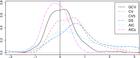
Obviously, negative values indicate undersmoothing ( smaller than , that is not enough bias reduction) while positive values indicate oversmoothing. The results remain essentially unchanged over the range of starting values, regression function and smoothers types we considered in our simulation study.
For small data sets (), the stopping rule based on data splitting produced values for that were very variable. A similar observation about the variability of bandwidth selection from data splitting was made in (see Hengartner et al., 2002). We also found that the five fold cross validation stopping rule produced highly variable values for .
The AIC stopping rule selects values that are often too big (oversmoothing) and sometimes selects the largest possible value of . In that cases, the curve versus (not shown) indicates two minimum, a local one which is around the true value and the global one at the boundary. This can be attributed to the fact that the penalty term used by AIC is too small. The AICc criteria uses a larger penalty term, which leads to smaller values for . In fact, the selected values are typically smaller than the optimal one. The penalty associated with GCV lies in between the AICc penalty and AIC penalty, and produces in practice values of that are closer to the optimum than either AIC or AICc. Finally, the leave one out cross-validation selection rule produces that are typically larger than the optimal one.
Investigation of the MSE as a function of the number of iterations reveal that, in the examples we considered, that function decreases rapidly towards its minimum and then remains relatively flat over a range of values to right of the minimum. It follows that the loss of stopping after is less than stopping before . We verify this empirically as follows: for each estimate, we calculate the approximation to the integrated mean squared error between the estimator and the true regression function
where is a fix grid of 100 regularly spaced points in the unit interval . We partition the calculated integrated mean squared error depending on whether is bigger than or smaller than . Figure 8 presents the boxplot of the integrated mean squared error when over-estimates and when it under-estimates and clearly shows that over-estimating leads to smaller integrated mean squared error than under-estimating .

For bigger data sets, say or bigger, most of the stopping criterion act the same except for the modified AIC which tends to select a smaller number of iterations than the ideal one. One fold cross-validation is rather computational intensive as the usual relation between cross validated estimator at and full data estimator is no longer valid (e.g. Hastie and Tibshirani, 1995, p. 47).
These conclusions remain true for kernel smoother and nearest neighbor smoothers. However if the pilot smoother is not smooth enough (not biased enough), then the number of iteration is too small to allow us to discriminate between the different stopping rules. These initial smoothers we name as wiggly learner are almost unbiased and therefore, there is little value to apply an iterative bias correction scheme. In conclusion, for small data sets, our simulations show that both GCV and leave one cross-validation work well, and for bigger data sets, we recommend using GCV.
Tables (1) and (2) here below report the finite sample performance of stopped boosted smoother by the GCV criterion. Each entry in the table reports the median number of iterations and the median mean square error over 100 simulations. As expected, larger smoothing parameter of the initial smoother require more iterations of the boosting algorithm to reach its optimum. Interestingly, the selected smoother starting with a very smooth smoother, has slightly smaller mean squared error. The quantify the benefits of the iterative bias correction scheme, the last column of the tables gives the mean squared error of the original smoother with smoothing parameters selected using GCV. In all cases, the iterative bias correction has smaller mean squared error than the ”one-step” smoother, with improvements ranging from 15% to 30%.
Table (1) presents the results for smoothing splines.
| Function | |||||||
|---|---|---|---|---|---|---|---|
| error | 1 | ||||||
| Gaussian | 4077 | 0.0273 | 65 | 0.0282 | 2 | 0.0293 | 0.0379 |
| student | 4115 | 0.0273 | 70 | 0.0286 | 2 | 0.0296 | 0.0352 |
| Function | |||||||
| Gaussian | 1219 | 0.0798 | 21 | 0.0845 | 1 | 0.0837 | 0.0829 |
| student | 1307 | 0.0887 | 22 | 0.0944 | 1 | 0.0932 | 0.0937 |
| Function | |||||||
| Gaussian | 135 | 0.0014 | 3 | 0.0014 | 1 | 0.0016 | 0.0016 |
| student | 147 | 0.0016 | 3 | 0.0016 | 1 | 0.0018 | 0.0019 |
Table (2) presents the results for kernel smoothers with a Gaussian kernel.
| Function | |||||||
|---|---|---|---|---|---|---|---|
| error | 1 | ||||||
| Gaussian | 385 | 0.0231 | 27 | 0.0254 | 4 | 0.0368 | 0.04857 |
| student | 360 | 0.0221 | 25 | 0.0262 | 4 | 0.0353 | 0.05199 |
| Function | |||||||
| Gaussian | 330 | 0.0477 | 128 | 0.0581 | 14 | 0.0782 | 0.1175 |
| student | 1621 | 0.0563 | 160 | 0.0660 | 16 | 0.0754 | 0.1184 |
| Function | |||||||
| Gaussian | 30 | 0.0017 | 7 | 0.0016 | 2 | 0.0014 | 0.00178 |
| student | 29 | 0.0017 | 8 | 0.0016 | 2 | 0.0016 | 0.0018 |
The simulation results reported in the above tables show that the iterative bias reduction scheme works well in practice, even for moderate sample sizes. While starting with a very smooth pilot requires more iterations, the mean squared error of the resulting smoother is somewhat smaller compared to a more noisy initial smoother. Figures 5 and 6 also support this claim.
7 Discussion
In this paper, we make the connection between iterative bias correction and the boosting algorithm, thereby providing a new interpretation for the latter. A link between bias reduction and boosting was suggested by Ridgeway (2000) in his discussion of the seminal paper Friedman et al. (2000), and explored in Di Marzio and Taylor (2004, 2007) for the special case of kernel smoothers. In this paper, we show that this interpretation holds for general linear smoothers.
It was surprising to us that not all smoothers were suitable to be used for boosting. We show that many weak learners, such as the -nearest neighbor smoother and some kernel smoothers, are not stable under boosting. Our results extend and complement the recent results of Di Marzio and Taylor (2007).
Iterating the boosting algorithm until convergence is not desirable. Better smoothers result if one stops the iterative scheme. We have explored, via simulations, various data driven stopping rules and have found that for the linear smoothers, the Generalized Cross Validation criteria works very well, even for moderate sample sizes of . In our simulations show that optimally correcting the bias (by stopping the boosting algorithm after a suitable number of iterations) produced better smoothers than the one with the best data-dependent smoothing parameter.
Finally, the iterative bias correction scheme can be readily extended to multivariate covariates , as in Buhlmann (2006).
Appendix A Appendix
Proof of Theorem 2.1 To show 2.5, let . The conclusion follows from a telescoping sum argument applied to
Proof of Theorem 2.3
where the last inequality follows from the assumptions on the spectrum of . Similarly, one shows that
Proof of Theorem 3.1 To simplify the exposition, let us assume that the ’s are ordered. Let us consider the -nn smoother the matrix is of general term
In order to bound the singular values of , consider the eigen values of which are the square of the singular values of . Since is symmetric, we have for any vector that
| (A.1) |
Let us find a vector such that . First notice that
Next, consider the vector of that is zero every where except at position (respectively and ) where its value is -1 (respectively 2 and -1). For this choice, we expand to get
To show that this last quantity is larger than , we need to suitably bound the off-diagonal elements of . To bound , where and , we need to consider three cases:
-
1.
If belongs to the -nn of and vice versa, then . This does not mean that all the -nn neighbor of are the same as those of , but if it is the case, then and otherwise in the pessimistic case, we bound . It therefore follows that
-
2.
If belongs to the -nn of but does not belong to the -nn of then . There is at a maximum of points that are in the -nn of and in the -nn of so . In the pessimistic case, there is only one point, which leads to the bound
-
3.
If does not belong to the -nn of and does not belong to the -nn of then . However there are potentially as many as points that are in the -nn of and in the -nn of , so that . In that case
With these bounds for the off-diagonal terms, we are able to major .
Before continuing, we need to discuss the relative position of the points and . We chose them such that
For this choice, we calculate
so that
The latter shows that whenever
which is always true if the condition
is satisfied because in such case, we have
Proof of Theorem 3.2 Let is an i.i.d. sample from a density that is bounded away from zero on a compact set strictly included in the support of . Consider without loss of generality that for all .
We are interested in the sign of the quadratic form where the individual entries of matrix are equal to
Recall the definition of the scaled kernel . If is the vector of coordinate then we have , where is the matrix with individual entries . Thus any conclusion on the quadratic form carry on to the quadratic form .
To show the existence of a negative eigenvalue for , we seek to construct a vector for which we can show that the quadratic form
converges in probability to a negative quantity as the sample size grows to infinity. We show the latter by evaluating the expectation of the quadratic form and applying the weak law of large number.
Let be a real function in , define its Fourier transform
and its Fourier inverse by
For kernels that are real symmetric probability densities, we have
From Bochner’s theorem, we know that if the kernel is not positive definite, then there exists a bounded symmetric set of positive Lebesgue measure (denoted by ), such that
| (A.2) |
Let be a real symmetric function supported on , bounded by (i.e. ). Obviously, its inverse Fourier transform
is integrable and by virtue of Parceval’s identity
Using the following version of Parceval’s identity (see Feller, 1966, p.620)
which when combined with equation (A.2), leads us to conclude that
Consider the following vector
With this choice, the expected value of the quadratic form is
We bound the first integral
Observe that for any fixed value , the latter can be made arbitrarily small by choosing large enough. We evaluate the second integral by noting that
| (A.3) | |||||
By virtue of the dominated convergence theorem, the value of the last integral converges to as goes to zero. Thus for small enough, (A.3) is less than zero, and it follows that we can make by taking , for some large . Finally, convergence in probability of the quadratic form to its expectation is guaranteed by the weak law of large numbers for statistics (see Grams and Serfling (1973) for example). The conclusion of the theorem follows.
Proof of Proposition 3.3 We are interested in the sign of the quadratic form (see proof of Theorem 3.2). Recall that if is semidefinite then all its principal minor (see Horn and Johnson, 1985, p.398) are nonnegative. In particular, we can show that is non-positive definite by producing a principal minor with negative determinant. To this end, take the principal minor obtained by taking the rows and columns . Without loss of generality, let us assume that . The determinant of is
Let us evaluate this quantity for the uniform and Epanechnikov kernels.
Uniform kernel. Let be larger than the minimum
distance between three consecutive points, and chose the index
such that
With this choice, we readily calculate
Since a principal minor of is negative, we conclude that
and are not semidefinite positive.
Epanechnikov kernel. For fixed,
denote by and by
, and assume that
. The determinant is
a bivariate function of and (as ).
Numerical evaluations of that function show that as soon
as we have the range of the three points less than the bandwidth,
the determinant of is negative.

Thus a principal minor of is negative, and as a result, and are not semidefinite positive.
References
- Akaike [1973] H. Akaike. Information theory and an extension of the maximum likelihood principle. In B. N. Petrov and B. F. Csaki, editors, Second international symposium on information theory, pages 267–281, Budapest, 1973. Academiai Kiado.
- Breiman [1998] L. Breiman. Arcing classifier (with discussion). Ann. of Statist., 26:801–849, 1998.
- Buhlmann [2006] P. Buhlmann. Boosting for high-dimensional linear models. Ann. of Statist., 34:559–583, 2006.
- Buhlmann and Yu [2003] P. Buhlmann and B. Yu. Boosting with the loss: Regression and classification. J. Amer. Statist. Assoc., 98:324–339, 2003.
- Buja et al. [1989] A. Buja, T. Hastie, and R. Tibshirani. Linear smoothers and additive models. Ann. of Statist., 17:453–510, 1989.
- Cleveland [1979] W. Cleveland. Robust locally weighted regression and smoothing scatterplots. J. Amer. Stat. Ass., 74:829–836, 1979.
- Craven and Wahba [1979] P. Craven and G. Wahba. Smoothing noisy data with spline functions. Numerische Mathematik, 31:377–403, 1979.
- Di Marzio and Taylor [2004] M. Di Marzio and C. Taylor. Boosting kernel density estimates: a bias reduction technique ? Biometrika, 91:226–233, 2004.
- Di Marzio and Taylor [2007] M. Di Marzio and C. Taylor. Multiple kernel regression smoothing by boosting. submitted, 2007.
- Di Marzio and Taylor [2008] M. Di Marzio and C. Taylor. On boosting kernel regression. to appear in JSPI, 2008.
- Efron et al. [2004] B. Efron, T. Hastie, I. Johnstone, and R. Tibshirani. Least angle regression (with discussion). Ann. of Statist., 32:407–451, 2004.
- Eubank [1988] R. Eubank. Spline Smoothing and Nonparametric Regression. Marcel Dekker, New-York, 1988.
- Fan and Gijbels [1996] J. Fan and I. Gijbels. Local Polynomial Modeling and Its Application, Theory and Methodologies. Chapman et Hall, New York, 1996.
- Feller [1966] W. Feller. An introduction to probability and its applications, volume 2. Wiley, New York, 1966.
- Freund [1995] Y. Freund. Boosting a weak learning algorithm by majority. Information and Computation, 121:256–285, 1995.
- Friedman [2001] J. Friedman. Greedy function approximation: A gradient boosting machine. Ann. Statist., 28(337-407), 2001.
- Friedman et al. [2000] J. Friedman, T. Hastie, and R. Tibshirani. Additive logistic regression: a statistical view of boosting. Ann. of Statist., 28:337–407, 2000.
- Grams and Serfling [1973] W. Grams and R. Serfling. Convergence rates for u-statistics and related statistics. Annals of Statistics, 1:153–160, 1973.
- Hastie and Tibshirani [1995] T. Hastie and R. Tibshirani. Generalized Additive Models. Chapman & Hall, 1995.
- Hengartner and Matzner-Løber [2007] N. Hengartner and E. Matzner-Løber. Asymptotic unbiased density estimators. accepted in ESAIM, 2007.
- Hengartner et al. [2002] N. Hengartner, M. Wegkamp, and E. Matzner-Løber. Bandwidth selection for local linear regression smoothers. JRSS B, 64:1–14, 2002.
- Hjort and Glad [1995] N. Hjort and I. Glad. Nonparametric density estimation with a paramteric start. Ann. Statist., 23:882–904, 1995.
- Horn and Johnson [1985] R. A. Horn and C. R. Johnson. Matrix analysis. Cambridge, New York, 1985.
- Hurvich et al. [1998] C. Hurvich, G. Simonoff, and C. L. Tsai. Smoothing parameter selection in nonparametric regression using and improved akaike information criterion. J. R. Statist. Soc. B, 60:271–294, 1998.
- Jones et al. [1995] M. Jones, O. Linton, and J. Nielsen. A simple and effective bias reduction method for kernel density estimation. Biometrika, 82:327–338, 1995.
- Li [1985] K. Li. From stein’s unbiased risk estimate to the method of generalized cross validation. Ann. Statist., 13:1352–1377, 1985.
- Li [1987] K.-C. Li. Asymptotic optimality for , , cross-validation and generalized cross-validation: Discrete index set. The Annals of Statistics, 15:958–975, 1987.
- Mallows [1973] C. L. Mallows. Some comments on . Technometrics, 15:661–675, 1973.
- Nadaraya [1964] E. Nadaraya. On estimating regression. Theory Probability and their Applications, 9(134-137), 1964.
- Ridgeway [2000] G. Ridgeway. Additive logistic regression: a statistical view of boosting: Discussion. Ann. of Statist., 28:393–400, 2000.
- Schapire [1990] R. Schapire. The strength of weak learnability. Machine learning, 5:197–227, 1990.
- Schwartz [1993] L. Schwartz. Analyse IV applications à la théorie de la mesure. Hermann, Paris, 1993.
- Schwarz [1978] G. Schwarz. Estimating the dimension of a model. Annals of statistics, 6:461–464, 1978.
- Simonoff [1996] J. Simonoff. Smoothing Methods in Statistics. Springer, New York, 1996.
- Tukey [1977] J. Tukey. Explanatory Data Analysis. Addison-Wesley, 1977.
- Utreras [1983] F. Utreras. Natural spline functions, their associated eigenvalue problem. Numer. Math., pages 107–117, 1983.
- Wahba [1990] G. Wahba. Spline models for observational data. SIAM, Philadelphia, 1990.
- Watson [1964] G. Watson. Smooth regression analysis. Sankhya A, 26(359-372), 1964.
- Whittaker [1923] E. Whittaker. On a new method of graduation. Proc. Edinburgh Math; Soc., 41:63–75, 1923.