Modeling Bell’s Non-resonant Cosmic Ray Instability

Abstract

We have studied the non-resonant streaming instability of charged energetic particles moving through a background plasma, discovered by Bell bell04 (2004). We confirm his numerical results regarding a significant magnetic field amplification in the system. A detailed physical picture of the instability development and of the magnetic field evolution is given.

1 Introduction

The diffusive shock acceleration process (Krymsky krymsky77 (1977); Axford et al. axford77 (1977); Bell bell78 (1978); Blandford and Ostriker blandford78 (1978)) is considered as the principal mechanism for the production of the galactic cosmic rays in supernova remnants (SNRs). A great strength of the random magnetic fields that provide the scattering of energetic particles both upstream and downstream of a supernova shock is necessary for efficient acceleration. It was originally suggested that this may be the result of a gyroresonant streaming instability that develops due to the presence of a diffusive streaming of accelerated particles (Bell bell78 (1978), Blandford & Ostriker blandford78 (1978)). The corresponding magnetohydrodynamic (MHD) waves have wavelengths of the order of the gyroradii of the energetic particles. This kind of resonant cyclotron instability had been suggested earlier to regulate the propagation of the galactic cosmic rays (Lerche lerche67 (1967), Wentzel wentzel74 (1974)). If the generated random fields are amplified up to wave amplitudes that correspond to the strength of the mean magnetic field, the scattering mean free path of resonant energetic particles will decrease to a value comparable with their gyroradius. This regime of diffusion is called Bohm diffusion and is often used to estimate the maximum energy of the accelerated particles.

However, even this rather optimistic regime of diffusion may ensure the acceleration of cosmic ray protons only up to energies of about $10^{14}$ eV (Lagage & Cesarsky lagage83 (1983), Berezhko ber96 (1996)) if the magnetic field in the remnant is comparable with the interstellar magnetic field, which is typically less than $10$ $\mu$G. Significant magnetic field amplification is necessary for acceleration up to higher energies. Amplification might be possible since quasilinear theory of the resonant streaming instability allows it (see e.g. McKenzie & Völk mckenzie82 (1982)). Since this perturbation theory breaks down in the case of resonant interaction of particles with high amplitude MHD waves, Lucek and Bell lucek00 (2000) performed MHD simulations combined with calculations of energetic particle trajectories and found that the magnetic field can be amplified to a level where the random field exceeds the initial mean field. The necessity to perform detailed trajectory calculations leads to strong numerical limitations of such simulations.

Different qualitative treatments of magnetic field amplification at supernova shocks were suggested on an analytical level (see e.g. Bell & Lucek bell01 (2001), Ptuskin & Zirakashvili ptuskin03 (2003), Vladimirov et al. vladimirov06 (2006), Amato & Blasi amato06 (2006)). Using the observed synchrotron emission, field amplification was included on a phenomenological level in numerical solutions of the coupled gas dynamic and particle acceleration equations (e.g. Berezhko et al. berezhko02 (2002), Berezhko & Völk 2004a ; 2004b , Völk et al. voelk07 (2007)). It became clear that such amplification can lead to particle accelaration to knee energies at $\approx 3\cdot 10^{15}$ eV and – according to speculative extrapolations – possibly even beyond.

On the basis of the dispersion relation for collisionless MHD waves derived by Achterberg achterberg83 (1983), Bell bell04 (2004) found a non-resonant streaming instability that had been overlooked before. He argued that the diffusive streaming of particles accelerated at supernova shocks may be so strong that it modifies the dispersion relation of MHD waves in an essential way. Then a non-oscillatory purely growing MHD mode appears at scales smaller than the gyroradius of the particles which excite the instability. The growth rate of this mode can be larger than the growth rate of the resonant mode. Since the particle trajectories are only weakly deflected by small-scale magnetic inhomogeneities, one can avoid complicated trajectory calculations. Only the mean cosmic-ray flux needs to be specified. Bell bell04 (2004) performed corresponding MHD simulations and showed that the magnetic field can indeed be significantly amplified.

In the following we investigate this non-resonant instability in considerably more detail. We have performed MHD simulations of the instability with very good numerical resolution and have found a simplified analytical description for the magnetic field amplification. Our results may be applied to different astrophysical objects, where energetic particles exist.

The present work deals with the instability in the presence of a non-resonant energetic particle population streaming through the thermal plasma. And it simulates the nonlinear instability development. In a companion paper (Zirakashvili & Ptuskin zirakashvili08 (2008), Paper II) this modeling will be combined with an analytical treatment of the diffusive acceleration of particles in a plane, steady shock with its intrinsically non-uniform energetic particle distribution in the precursor.

The paper is organized as follows: The basic equations are given in the next section. The scattering of cosmic ray particles by small-scale random magnetic fields is considered in Sect.3. The cosmic ray electric current is calculated in Sect. 4. The non-resonant instability and the MHD simulations are described in Sect.5 and 6. The summary is given in the last Section.

2 Basic equations

We consider a system that consists of a thermal plasma and a cosmic ray gas with a negligible mass density. We shall treat the gas as a magnetized fluid with frozen-in magnetic field ${\bf B}$ and induced electric field ${\bf E=-[u\times B]}/c$. Here ${\bf u}$ is the mass velocity (essentially equal to the thermal gas velocity) and $c$ is the velocity of light. The electric charge density $\rho_{\mathrm{th}}$ and electric current density ${\bf j}_{\mathrm{th}}$ of the thermal plasma that determine the Lorentz force ${\bf F}=[({\bf j}_{\mathrm{th}}-\rho_{\mathrm{th}}{\bf u})\times{\bf B}]/c$ may be found from the quasi-neutrality condition $\rho_{\mathrm{th}}=-\rho_{\mathrm{cr}}$ and Ampère’s law $[\nabla\times{\bf B}]=4\pi({\bf j}_{\mathrm{th}}+{\bf j}_{\mathrm{cr}})/c$, respectively. Here $\rho_{\mathrm{cr}}$ and ${\bf j}_{\mathrm{cr}}$ are the electric charge density and electric current density of the cosmic ray gas, respectively. The Euler equation of the gas motion may then be written as

$$\rho\left(\frac{\partial{\bf u}}{\partial t}+({\bf u\nabla)u}\right)=-\frac{[\bf B\times[\nabla\times B]]}{4\pi}-\nabla P$$

$$-\frac{1}{c}[({\bf j}_{\mathrm{cr}}-\rho_{\mathrm{cr}}{\bf u})\times{\bf B}],$$ (1)

where $P$ is the thermal gas pressure.

The evolution of the mass density $\rho$ and the magnetic field ${\bf B}$ are governed by the continuity equation

$$\frac{\partial\rho}{\partial t}+\nabla(\rho{\bf u})=0$$ (2)

and Faraday’s law

$$\frac{\partial{\bf B}}{\partial t}=[\nabla\times[{\bf u}\times{\bf B}].$$ (3)

The equation for the plasma energy density $e=(\rho{u^{2}}/2)+(B^{2}/(8\pi))+P/(\gamma-1)$ may be written as:

$$\frac{\partial e}{\partial t}+\nabla\left(\rho{\bf u}\frac{u^{2}}{2}+\frac{\gamma P{\bf u}}{\gamma-1}+\frac{[{\bf B\times[u\times B]}}{4\pi}\right)$$

$$=-\frac{\bf u}{c}[{\bf j}_{\mathrm{cr}}\times{\bf B}].$$ (4)

Here $\gamma$ is the adiabatic index of the gas. The last term in this equation describes the mechanical work produced by cosmic rays. The electric charge density $\rho_{\mathrm{cr}}$ and the electric current density of cosmic rays ${\bf j}_{\mathrm{cr}}$ may be found from the momentum distribution of cosmic rays $f({\bf p,r},t)$. It obeys the equation

$$\frac{\partial f}{\partial t}+{\bf v}\nabla f+\frac{q}{c}[({\bf v}-{\bf u})\times{\bf B}]\frac{\partial f}{\partial{\bf p}}=0.$$ (5)

Here $q$ is the charge of cosmic ray particles.

The system of Eqs. (1)-(5) describes the interaction of cosmic rays and magnetized thermal plasma. We shall use this system in the next sections.

3 Scattering by the small-scale field

The cosmic ray momentum distribution may be written as $f=f_{0}+\delta f$. Here $f_{0}=\left<f\right>$ is the momentum distribution averaged over the fluctuations of the magnetic field $\delta{\bf B}$ and of the plasma velocity $\delta{\bf u}$; $\delta f$ is the fluctuation of the momentum distribution. One can use perturbation theory for the calculation of $\delta f$ when the fluctuations of the magnetic field are small in comparison with the mean field ${\bf B}_{0}$. Since we are interested in the investigation of considerable magnetic field amplification, the theory of perturbations with small magnetic field amplitude is, generally speaking, not applicable. Fortunately in the case of the non-resonant instability that is most interesting for the present consideration, only small-scale fields are generated (see also below) and the scale of the random field is smaller than the particle gyroradius in the total magnetic field. Perturbation theory is applicable in this case because the particles are only weakly deflected on the characteristic scale of the random field. The theory of cosmic ray diffusion in such magnetic fields was developed by Dolginov and Toptygin dolginov67 (1967).

The equation for the fluctuation of the momentum distribution can be found from Eq. (5):

$$\frac{\partial\delta f}{\partial t}+{\bf v}\nabla\delta f+\frac{q}{c}[({\bf v}-{\bf u}_{0})\times{\bf B}_{0}]\frac{\partial\delta f}{\partial{\bf p}}$$

$$=-\frac{q}{c}[({\bf v}-{\bf u}_{0})\times{\bf\delta B}]\frac{\partial f_{0}}{\partial{\bf p}}.$$ (6)

Here ${\bf u}_{0}$ is the mean mass velocity and we neglect the velocity perturbations $\delta{\bf u}$. It is assumed that they are small in comparison with the mean velocity ${\bf u}_{0}$. Such perturbations would only result in second order Fermi acceleration which is a factor of $\left<\delta u^{2}\right>/c^{2}$ slower in comparison with particle scattering.

Since the random field ${\bf\delta B}$ has small spatial scales, the last term on the left-hand side of this equation may be also neglected. This means that to lowest order the particles can be considered to move in straight-line orbits. The calculations are in this case significantly simplified in comparison with the general case, when the integration along the helical orbits of particles results in the appearance of series containing Bessel functions (see e.g. Berezinskii et al. berezinsky90 (1990)). Although the zero-order orbits are different for these two methods, they give similar results in the case of almost any small-scale random magnetic field. The formal limit $B_{0}\to 0$ is not trivial and was considered by Tsytovich tsytovich77 (1977).

As long as the gradient lengths of $f_{0}$ and ${\bf u}_{0}$ are large compared to the spatial fluctuation scale $k^{-1}$, the fluctuation amplitudes carry a corresponding parametrical spatial dependence. We shall assume this in the following. Fourier transforming then in time and space we find the expression for the Fourier transform of the distribution $\delta f_{\omega,{\bf k}}=\int d^{3}rdt\delta f\exp(i(\omega t-{\bf kr}))(2\pi)^{-4}$:

$$\delta f_{\omega,{\bf k}}=\frac{q/c}{i(\omega-{\bf kv})}[({\bf v}-{\bf u}_{0})\times{\bf\delta B_{\omega,k}}]\frac{\partial f_{0}}{\partial{\bf p}}.$$ (7)

Here ${\bf\delta B_{\omega,k}}$ is the Fourier transform of the random magnetic field. We shall further assume that the magnetic field changes slowly in time in the frame moving with the mean mass velocity ${\bf u}_{0}$ and therefore write ${\bf\delta B_{\omega,k}}=\delta{\bf B_{k}}\delta(\omega-{\bf ku}_{0})$.

Averaging now Eq. (5) and using Eq.(7) we obtain the following kinetic equation for the average cosmic ray distribution function $f_{0}$:

$$\frac{\partial f_{0}}{\partial t}+{\bf v}\nabla f_{0}+q\left({\bf E}_{0}+\frac{1}{c}[({\bf v}-{\bf u}_{0})\times{\bf B}_{0}]\right)\frac{\partial f_{0}}{\partial{\bf p}}$$

$$=\frac{\partial}{\partial p_{i}}\nu_{ij}\frac{\partial f_{0}}{\partial p_{j}}$$ (8)

Here ${\bf E}_{0}=-c^{-1}\left<\bf\delta u\times\delta B\right>$ is the mean electric field in the frame of reference moving with the mean plasma velocity ${\bf u}_{0}$.

The scattering tensor $\nu_{ij}$ in the last equation is determined by the spectrum of the random magnetic field $B_{ij}({\bf k})=\int\frac{d^{3}r}{(2\pi)^{3}}\left<B_{i}{\bf(r+r}_{0})B_{j}{\bf(r}_{0})\right>\exp(-i{\bf kr)}$:

$$\nu_{ij}=\frac{q^{2}}{c^{2}}\pi\int d^{3}k\delta({\bf k(v-u}_{0}))e_{ilm}e_{jrs}$$

$$\times B_{lr}({\bf k})(v_{m}-u_{0m})(v_{s}-u_{0s})$$ (9)

Here $e_{ijk}$ is the antisymmetric tensor. The scattering tensor makes the cosmic ray distribution isotropic in the frame moving with the velocity ${\bf u}_{0}$. Expression (9) may be simplified in the case of an isotropic random magnetic field $B_{ij}({\bf k})=\frac{1}{2}B_{\mathrm{isotr}}(k)(\delta_{ij}-k_{i}k_{j}/k^{2})$ (Dolginov & Toptygin dolginov67 (1967)):

$$\nu_{ij}=p^{2}\nu(p)\frac{({\bf v-u_{0}})^{2}\delta_{ij}-(v_{i}-u_{0i})(v_{j}-u_{0j})}{2v|{\bf v-u}_{0}|}$$ (10)

where the scattering frequency $\nu(p)$ is given by the formula

$$\nu(p)=\frac{\pi}{4}\frac{q^{2}v}{p^{2}c^{2}}\int d^{3}kB_{\mathrm{isotr}}(k)/k$$ (11)

Here the spectrum of the isotropic magnetic field is normalized as $\left<\delta B^{2}\right>=\int d^{3}kB_{\mathrm{isotr}}(k)$.

In the diffusion approximation the average cosmic ray distribution function $f_{0}$ may be written as

$$f_{0}({\bf p})=N(p)+\frac{3}{pv}{\bf pJ}(p),$$ (12)

where $N(p)$ is the isotropic part and ${\bf J}(p)$ is the cosmic ray flux density, which is the sum of the diffusive and advective flux densities and is given by Eq. (A.3) in Appendix A.

4 Calculation of the electric current

We shall use Eq. (7) for the calculation of the electric current density of the cosmic ray gas. Substitution of the expression (12) into Eq. (7), multiplication by $q{\bf v}$, and integration over momentum space give the fluctuating part of the Fourier transform of the cosmic ray electric current $\delta{\bf j}_{\mathrm{cr,\omega,{\bf k}}}$. Disregarding terms of the order $u_{0}/v$ we obtain

$$\delta{\bf j}_{\mathrm{cr,\omega,{\bf k}}}=3\pi\frac{q^{2}}{c}\delta(\omega-{\bf ku}_{0})\int\frac{d^{3}p}{pv}\delta({\bf kv)(J}_{\mathrm{d}}[{\bf v\times\delta B_{k}])v}.$$ (13)

Here ${\bf J}_{\mathrm{d}}={\bf J+u}_{0}\frac{p}{3}\frac{\partial N}{\partial p}$ is the average cosmic ray diffusion flux. The appearance of the $\delta$-function in this equation is due to the Landau resonance $\omega={\bf kv}$ (cf. Lifshitz and Pitaevskii lifshitz81 (1981)) in Eq.(7).

The total electric current of the cosmic ray gas is the flux $\bf J$ multiplied by the particle charge $q$.

Performing the integration on the two angles in momentum space, and calculating the inverse Fourier transformation of the last equation, we obtain the expression for the diffusive electric current ${\bf j}_{\mathrm{d}}={\bf j}_{\mathrm{cr}}-\rho_{\mathrm{cr}}{\bf u}$ that appears in the right-hand side of Eq. (1):

$${\bf j}_{\mathrm{d}}=q\int d^{3}p{\bf J}_{\mathrm{d}}+\frac{3\pi}{4}\frac{q^{2}}{c}\int d^{3}k\exp(i{\bf k(r-u}_{0}t))$$

$$\times\int\frac{d^{3}p}{pk^{3}}\left(k^{2}{\bf[\delta B_{k}\times J}_{\mathrm{d}}]-{\bf k(k[\delta B_{k}\times J}_{\mathrm{d}}])\right).$$ (14)

The first term on the right-hand-side of this equation is simply the zero-order term of the expansion in the magnetic fluctuation $\delta{\bf B}$, while the second term is the linear term of the expansion. The latter is always smaller than the first term if the small-scale field approximation is valid, that is if $qB/pck<<1$, which means that the particle gyroradius $pc/qB$ is large compared to the scale $k^{-1}$ of the magnetic field.

However, in some cases the second integral may play a rôle. When the cosmic ray streaming is not strong, it results only in a small change of the dispersion relation of MHD waves. The first integral in Eq. (14) in this case produces only a small shift of the frequency of MHD waves. The second term then gives a small imaginary part of the frequency and describes a resonant wave instability based on the Landau resonance in Eq. (7). Within the limits of the small-scale field approximation, and for strong cosmic ray streaming, this resonant instability is ineffective in comparison to the well-known gyroresonant streaming instability.

Another important point is that the second integral on the right-hand side of Eq. (14) appears in the calculation of the mean force acting on the thermal plasma (Ptuskin ptuskin84 (1984)): ${\bf F}=c^{-1}\left<[{\bf B\times(\bf j}_{\mathrm{cr}}-\rho_{\mathrm{cr}}{\bf u}_{0})]\right>$.

Using Eq. (14) and averaging we obtain

$${\bf F}=\frac{\pi}{4}\frac{q^{2}}{c^{2}}\int\frac{d^{3}p}{p}{\bf J}_{d}\int d^{3}kB_{\mathrm{isotr}}(k)/k$$

$$=\int{d^{3}p}\frac{p}{v}\nu(p){\bf J}_{d}$$ (15)

It was assumed here that the random field is isotropic and expression (11) was used. Since the diffusive flux is equal to ${\bf J}_{d}=-\frac{v^{2}}{3\nu}\nabla N$ in the diffusion approximation, ${\bf F}=-\nabla P_{\mathrm{cr}}$, where $P_{\mathrm{cr}}=\int d^{3}ppvN(p)/3$ is the cosmic ray pressure. In the sense of MHD theory, Eq. (1) then describes the overall momentum balance of the system, where the forces on the r.h.s. are the Lorentz force and the gradient of the overall pressure, thermal plus nonthermal. Indeed $c^{-1}\left<[({\bf j}_{\mathrm{cr}}-\rho_{\mathrm{cr}}{\bf u}_{0})\times{\bf B}]\right>=-\nabla P_{\mathrm{cr}}$ is the general form of the average cosmic ray momentum balance.

In the sequel we will neglect the 2nd term of Eq. (14) (see also Bell bell04 (2004)). This is justified in the linear analysis and in the nonlinear simulation of the non-resonant instability if the small-scale field approximation is valid.

Figure 1: Explanation of the non-resonant streaming instability. The magnetic spiral (thin solid line) is stretched by the Lorentz force ${\bf F}=-[{\bf j}_{\mathrm{d}}\times{\bf B}]c^{-1}$ that appears due to the diffusive cosmic ray electric current ${\bf j}_{\mathrm{d}}$.

5 Non-resonant streaming instability

The dispersion relation for small-scale MHD perturbations may be found from Eqs. (1)-(5). In the case when the cosmic ray diffusion flux ${\bf J}_{\mathrm{d}}$ and the wavenumber ${\bf k}$ are parallel to the mean magnetic field ${\bf B}_{0}$ this dispersion relation may be written as (Bell bell04 (2004)):

$$(\omega-{\bf ku}_{0})^{2}=V^{2}_{\mathrm{a}}k^{2}\mp\frac{j_{\mathrm{d}}B_{0}}{c\rho_{0}}k.$$ (16)

Here $\rho_{0}$ is the mean plasma density, $V_{\mathrm{a}}=B_{0}/\sqrt{4\pi\rho_{0}}$ is the Alfvén velocity, ${\bf j}_{\mathrm{d}}=q\int d^{3}p{\bf J}_{\mathrm{d}}$ is the average diffusive electric current of cosmic rays, and the two signs $\mp$ correspond to the two circular polarizations. A non-resonantly unstable MHD mode appears if the condition $k<k_{\mathrm{c}}=j_{\mathrm{d}}B_{0}/c\rho_{0}V^{2}_{\mathrm{a}}$ is fulfilled. The unstable magnetic field line spiral expands in the direction perpendicular to the mean magnetic field (see Fig.1). The mode with $k=k_{\mathrm{c}}/2$ has the maximum growth rate $\gamma_{\max}$ :

$$\gamma_{\max}=\frac{j_{\mathrm{d}}B_{0}}{2c\rho_{0}V_{\mathrm{a}}},$$ (17)

which does not depend on the magnetic field strength.

Since we assumed that the scale $k^{-1}$ of the perturbations is smaller than the gyroradius $pc/qB_{0}$ of the energetic particles, the wavenumber $k$ should obey the condition $qB_{0}/pc<<k_{\mathrm{c}}$. This means that the necessary condition for instability is $k_{\mathrm{c}}>qB_{0}/pc$. This condition may be rewritten as

$$\frac{u_{\mathrm{cr}}}{v}\frac{\epsilon_{\mathrm{cr}}}{B^{2}_{0}/4\pi}>>1$$ (18)

Here $u_{\mathrm{cr}}$ and $\epsilon_{\mathrm{cr}}$ are the bulk velocity and the energy density of the cosmic ray gas, respectively, and $v$ is the velocity of energetic particles. This condition is easily fulfilled at the shocks of SNRs, where $u_{\mathrm{cr}}$ is of the order of the shock velocity $u_{1}$ and the energy density of the relativistic particles may be comparable with $\rho u^{2}_{1}$.

Figure 2: Numerical results of the modeling of the non-resonant instability with the dimensionless cosmic ray electric current $J=16$ as a function of normalized time $\tilde{t}$. The r.m.s. values of the magnetic field fluctuation $\left<\delta B^{2}\right>^{1/2}$ divided by the mean magnetic field strength $B_{0}$ and of the mass velocity fluctuations $\left<\delta u^{2}\right>^{1/2}$ divided by the Alfvén velocity $V_{a}$ are shown by the solid and dashed lines, respectively. The ratio of the sonic velocity $c_{\mathrm{s}}$ and the Alfvén velocity $V_{a}$ is shown by the dotted line. The square root of the ratio of the mean electric field $E_{0}$ and the mean magnetic field $B_{0}$ multiplied on $(c/V_{a})^{1/2}$ is shown by the thin solid line. The characteristic scale $L_{m}$ of the magnetic field is also shown by the thin dashed line.

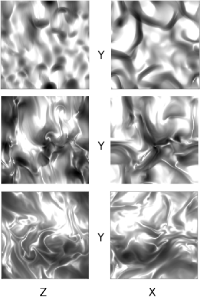
Figure 3: Slices of the magnetic field strength through the center of the box, obtained at $\tilde{t}=0.82$ (top), $\tilde{t}=1.03$ (middle) and $\tilde{t}=1.48$ (bottom), in the run with $J=16$. The scaling of the magnetic field strength is logarithmic between $0.32\left<B^{2}\right>^{1/2}$ (white) and $3.2\left<B^{2}\right>^{1/2}$ (black). The mean magnetic field and the diffusive electric current are in the $z$ direction.

6 Numerical modeling of the non-resonant instability

We have numerically modeled the non-resonant instability similar in spirit to the modeling of Bell bell04 (2004). The MHD Eqs. (1)-(4), written in dimensionless form, were solved numerically. We used the numerical method of Pen et al. pen03 (2003). It is a second order in space and time, flux-conservative total variation diminishing MHD scheme which enforces the $\nabla{\bf B}=0$ constraint to machine precision. The nonlinear flux limiter ”minmod” was used.

Figure 4: The one-dimensional spectra of the perpendicular component of the random magnetic field $B_{\perp}(\tilde{k}_{z})$ obtained at $\tilde{t}=0$ (thin solid line), $\tilde{t}=0.54$ (solid line), $\tilde{t}=0.74$ (dashed line), $\tilde{t}=0.97$ (dotted line) and $\tilde{t}=1.26$ (thick solid line). All spectra are normalized to the square of the mean magnetic field. The critical wavenumber $\tilde{k}_{c}=16$ is marked on the $x$-axis.

The dimensionless time $\tilde{t}$, the space coordinate $\tilde{z}$ and the velocity $\tilde{u}$ are defined as $\tilde{t}=tV_{\mathrm{a}}k_{0}$, $\tilde{z}=k_{0}z$, $\tilde{u}=u/V_{\mathrm{a}}$, respectively. Here $k_{0}$ is the wavenumber that corresponds to the real size of the numerical box $2\pi/k_{0}$. The dimensionless density $\tilde{\rho}$ and the electric current $J$ can be expressed via the magnetic field $B_{0}$ and the Alfvén velocity $V_{\mathrm{a}}$ as $\tilde{\rho}=4\pi\rho V_{\mathrm{a}}^{2}/B_{0}^{2}$ and $J=4\pi j/ck_{0}B_{0}$. The dimensionless wavenumber $\tilde{k}$ is simply $\tilde{k}=k/k_{0}$.

The simulations were performed in a cubic box with size $2\pi$. Periodic boundary conditions were imposed at the sides of the box. We used $256^{3}$ grid cells in our simulations (to be compared with $128^{3}$ cells in Bell’s case).

At $\tilde{t}=0$ the plasma pressure and density are uniformly distributed in space. Small random magnetic perturbations corresponding to isotropically distributed Alfvén waves with a one dimensional spectrum $\propto k^{-1}$ and $\left<B^{2}\right>^{1/2}/B_{0}=0.09$ were added to the mean unit strength magnetic field that is in $z$ direction. Here $\left<\right>$ denote the spatial average over the simulation volume. We use the values $\gamma=5/3$ and $\beta=1$. Here $\beta=4\pi P/B_{0}^{2}$.

The evolution of the magnetic field and the mass velocity fluctuations, together with the evolution of the sound speed, the mean electric field $E_{0}$ and the characteristic scale $L_{m}$ of the magnetic field, for a dimensionless cosmic ray current $J=16$, is shown in Fig.2. The characteristic scale $L_{m}=\int dk_{z}B_{\perp}(k_{z})|k_{z}|^{-1}/\int dk_{z}B_{\perp}(k_{z})$ is determined via the spectrum $B_{\perp}(k_{z})$ of the perpendicular component of the random magnetic field $B_{\perp}(k_{z})=\int dk_{x}dk_{y}(B_{xx}({\bf k})+B_{yy}({\bf k}))$.

After a brief initial stage the fluctuations grow exponentially with a growth rate that is slightly smaller than $\tilde{\gamma}_{\max}=8$ in dimensionless units. The initial growth of the magnetic fluctuations is not exponential, since only a part of the initial perturbation corresponds to unstable modes.

At $\tilde{t}=0.7$ the magnetic perturbations are already comparable with the mean magnetic field. Parts of the magnetic spiral expanding into the $XY$-plane begin to collide with their surroundings. When this happens multiple shocks are formed. The shape of these shocks may be seen in the top panel of Fig.3, where the magnetic field strength in perpendicular slices through the center of the box are shown. In the $YZ$-plane, which contains the initial magnetic field vector, they look like bow shocks. The shocks corresponding to the adjacent turns of the same magnetic spiral are clearly seen. These shocks are almost circular in the $XY$-plane. Low density cavities appear inside these shocks. The size of these cavities in the $XY$ plane is larger than the size in the $z$ direction. At later times the shocks collide with each other in the $XY$ plane and the gas motion becomes strongly turbulent (middle and bottom panels of Fig.3).

The MHD turbulence has rather small spatial scales in the early stage of the magnetic field growth. The scale of the magnetic field increases with time (see Fig.2). This increase is slower in comparison with what was suggested by Bell $k\sim 4\pi j_{\mathrm{d}}/Bc$ (or $\tilde{k}\sim JB_{0}/B$ in dimensionless units) when the magnetic tension forces are comparable with the Lorentz force produced by the cosmic ray electric current. This effect is illustrated in Fig.4, where the magnetic spectra obtained for several instants of time, are shown. It is clear from this figure that a nonlinear transfer of magnetic energy takes place in the system. The increase of the magnetic energy at wavenumbers $\tilde{k}>\tilde{k}_{c}$ that are not excited in the linear approximation demonstrates the non-linear transfer of energy to smaller scales. The magnetic energy in the small wavenumbers also grows faster than predicted by the analytical growth rate formula. For example the amplitude of the harmonics with wavenumber $\tilde{k}=1$ increases by a factor of 4.4 during the period from $\tilde{t}=0.74$ up to $\tilde{t}=0.97$ (see Fig.4). The linear growth rate for this harmonics $\tilde{\gamma}=\sqrt{J\tilde{k}-\tilde{k}^{2}}=\sqrt{15}$ corresponds to an amplification factor of about 2.2 during this period. This demonstrates the nonlinear transfer of energy to larger scales. Thus the magnetic energy is non-linearly transferred to both smaller and larger scales compared to the linearly excited spatial scales.

Towards the end of the simulation, at $\tilde{t}\sim 1.5$, the scale of the magnetic field is comparable with the size of the box. At this point in time the internal energy of the thermal gas is roughly equal to the kinetic and magnetic energy in our simulation. Bell continued his calculation beyond this point and found that at later times the magnetic field reaches a saturation value. Also continuing our simulations we found that the magnetic field continues to grow. We believe that this difference is due to the fact that different MHD codes were used. The difference is not important however, since the simulation does not model the real situation any more when the scale of the field has become comparable with the size of the spatial simulation domain. In this sense our results are similar to Bell’s results.

The growth of the MHD perturbations decreases with increasing magnetic field amplification. As estimated in Appendix B, the magnetic field is amplified only linearly at large times, $B/B_{0}\sim J\tilde{t}$ in dimensionless units, whereas the gas thermal energy density increases $\propto t^{3}$. These dependencies are derived using the equation for the evolution of the magnetic helicity.

7 Conclusion

We have modeled the non-resonant instability produced by a flux of charged energetic particles that is driven through a scattering thermal plasma. Using a significantly better numerical resolution we basically confirm the results obtained earlier by Bell bell04 (2004). The magnetic field may be amplified significantly. The unstable magnetic spirals collide with each other and shocks of moderate strength are formed as the instability develops (see previous Section). These shocks lead to significant gas heating. Since free expansion of the magnetic spirals after collision is impossible, the field grows only linearly in time at later epochs (see Eq. (B3)). If the system has enough time to evolve, the magnetic field growth will be stopped when the gyroradius $pc/qB$ of the energetic particles in the amplified field $B$ will drop down to the scale of the amplified field $k^{-1}\sim cB/4\pi j_{\mathrm{d}}$. This determines the value of the saturated magnetic field (Bell bell04 (2004), Pelletier et al. pelletier06 (2006)):

$$\frac{B^{2}}{4\pi}\sim\frac{u_{\mathrm{cr}}}{v}\epsilon_{\mathrm{cr}}.$$ (19)

We should note that the small-scale approximation considered in Sect. 3 becomes invalid when the magnetic field reaches this saturation value.

Since the instability is driven by the Lorentz force, the corresponding MHD turbulence has specific properties. It has non-zero magnetic helicity and a non-zero mean electric field ${\bf E}_{0}$ parallel to the mean magnetic field.

We expect that the formation of multiple shocks in three-dimensional MHD turbulence will also occur for other instabilities, in particular for the resonant streaming instability, driven by cosmic rays.

The scattering of energetic particles by the small-scale magnetic inhomogeneities can be described using the Dolginov-Toptygin approximation (Dolginov & Toptygin dolginov67 (1967)). The appearance of a mean second order electric field ${\bf E}_{0}=-c^{-1}\left<\bf\delta u\times\delta B\right>$, which is oppositely directed to the electric current of the energetic particles, modifies the cosmic ray transport equation (see Appendix A).

This non-resonant streaming instability may be important in any astrophysical site where a strong electric current of energetic particles exists and where the initial magnetic strength is small enough (see condition (18)). Supernova remnants, starburst galaxies, galaxy cluster accretion shocks and AGN jets are possible candidates for an application of this instability.

The results obtained will be used in a companion paper by Zirakashvili & Ptuskin zirakashvili08 (2008) (Paper II) for a model of diffusive shock acceleration in young SNRs in the presence of the non-resonant streaming instability.

Appendix A Diffusion approximation in the presence of the additional electric field

The cosmic ray transport equation is modified in the presence of the additional mean electric field ${\bf E}_{0}=-c^{-1}\left<\bf\delta u\times\delta B\right>$ (Fedorov et al. fedorov92 (1992)). Let us substitute the cosmic ray momentum distribution (12) into Eq. (8) with the scattering tensor (10). Performing the expansion up to the second order in $u/v$ and collecting the terms independent of the direction of the particle velocity ${\bf v}$ and separately those proportional to the velocity we obtain after some algebra

$$\frac{\partial N}{\partial t}+\nabla{\bf J}+\frac{1}{p^{2}}\frac{\partial}{\partial p}\frac{p^{2}}{v}q({\bf E}_{0}{\bf J})=\frac{{\bf u}_{0}}{p^{2}}\frac{\partial}{\partial p}\frac{p^{3}}{v^{2}}\left(\nu\left({\bf J+u}_{0}\frac{p}{3}\frac{\partial N}{\partial p}\right)+\left[{\bf\Omega\times J}\right]\right),$$ (A1)

$$\frac{\partial{\bf J}}{\partial t}+\frac{v^{2}}{3}\nabla N+q{\bf E}_{0}\frac{v}{3}\frac{\partial N}{\partial p}=-\nu\left({\bf J+u}_{0}\frac{p}{3}\frac{\partial N}{\partial p}\right)+\left[{\bf\Omega}\times\left({\bf J+u}_{0}\frac{p}{3}\frac{\partial N}{\partial p}\right)\right]$$ (A2)

Here ${\bf\Omega}=qv{\bf B}_{0}/pc$. Assuming a slow time evolution we neglect the time derivative in the last equation. Then it can be used to find the cosmic ray flux ${\bf J}$:

$$J_{i}=-D_{ij}\left(\nabla_{j}N+E_{0j}\frac{q}{v}\frac{\partial N}{\partial p}\right)-{u_{0i}}\frac{p}{3}\frac{\partial N}{\partial p},$$ (A3)

where the diffusion tensor $D_{ij}$ has the following form

$$D_{ij}=(D_{\parallel}-D_{\perp})b_{i}b_{j}+D_{\perp}\delta_{ij}+D_{A}e_{ijk}b_{k}.$$ (A4)

Here ${\bf b}={\bf B}_{0}/B_{0}$ is the unit vector in the direction of the mean field ${\bf B}_{0}$, $D_{\parallel}$ and $D_{\perp}$ denote the parallel and perpendicular diffusion coefficients, respectively, and $D_{A}$ is the antisymmetric diffusion coefficient. They are given by Dolginov & Toptygin dolginov67 (1967)):

$$D_{\parallel}=\frac{v^{2}}{3\nu},\ D_{\perp}=\frac{v^{2}\nu/3}{\Omega^{2}+\nu^{2}},\ D_{A}=\frac{v^{2}\Omega/3}{\Omega^{2}+\nu^{2}}.$$ (A5)

Then Eq. (A1) reduces to

$$\frac{\partial N}{\partial t}+{\bf u}_{0}\nabla N-\frac{p}{3}\frac{\partial N}{\partial p}\nabla{\bf u}_{0}=\left(\nabla_{i}+\frac{1}{p^{2}}\frac{\partial}{\partial p}\frac{p^{2}q}{v}E_{0i}\right)D_{ij}\left(\nabla_{j}N+\frac{q}{v}E_{0j}\frac{\partial N}{\partial p}\right).$$ (A6)

Eq. (A6) shows how the presence of the mean electric field ${\bf E}_{0}$ modifies the diffusion term of the cosmic ray transport equation.

Appendix B Magnetic helicity

As noted first by Pelletier et al. pelletier06 (2006), the MHD turbulence generated by the non-resonant instability has nonzero magnetic helicity $H=\left<\delta{\bf A}\delta{\bf B}\right>$, where $\delta{\bf A}$ is the perturbation of the magnetic potential. The magnetic helicity $H$ is a useful quantity and it is often used in the theory of MHD turbulence and dynamo theories (see e.g. Biskamp biskamp03 (2003)). Faraday’s equation (3) may be used for the determination of the time evolution of this quantity. For the periodic system we have (cf. Subramanian & Brandenburg subramanian04 (2004))

$$\frac{\partial H}{\partial t}=-2c{\bf B}_{0}{\bf E}_{0}$$ (B1)

We neglect magnetic dissipation here. This seems well justified because the magnetic helicity is an integral quantity and is not transferred by nonlinear interactions to smaller scales where dissipation is essential. In this sense the magnetic helicity is different from the nonthermal (kinetic + magnetic) energy that may be transferred to smaller and smaller scales where it is transformed into gas thermal energy even in the case of infinitely small viscosity.

The mean electric field appears in the system as a response of the medium to the cosmic ray electric current. The evolution of the energy density of the plasma takes place according to Eq. (4). The right-hand side of this equation is simply $-{\bf E}_{0}{\bf j}_{\mathrm{d}}$. Comparing with Eq. (B1) for a time independent $j_{\mathrm{d}}$, we obtain the relation

$$H-2\frac{B_{0}\left<e\right>}{j_{\mathrm{d}}}=\mathrm{const}(t)$$ (B2)

It is worth emphasizing that Eq. (B2) is valid for the total plasma energy density $e$ which appears in Eq. (4). During the stage of exponential growth the instability produces magnetic field and velocity perturbations, whereas gas heating is important at later times.

We may use Eq. (B1) for a derivation of the equation for the magnetic field amplification. Since the turbulence is helical, the magnetic helicity (that is the product of the magnetic field and the vector magnetic potential) is $H\sim B^{2}/k$, the electric field is $E_{0}\sim V_{\mathrm{a}}B^{2}/cB_{0}$, and $k\sim 4\pi j_{\mathrm{d}}/Bc$. Then Eq. (B.1) yields the equation for the amplification of the magnetic field:

$$\frac{\partial B}{\partial t}\sim\frac{4\pi V_{\mathrm{a}}j_{\mathrm{d}}}{c}$$ (B3)

The numerical factor in this equation is of order unity, according to our numerical results.

There is another way to obtain this last equation. The field is amplified by turbulent motions of the medium, that is $\partial B/\partial t\sim B_{0}ku_{k}$, where $u_{k}$ is the turbulent velocity with wavenumber $k$. Assuming equipartition, $u_{k}\sim V_{\mathrm{a}}B/B_{0}$, and the estimate $kB\sim 4\pi j_{\mathrm{d}}/c$, we arrive at Eq. (B3).

Since $H\propto B^{3}$ at late times, also $\left<e\right>\propto t^{3}$, cf. Eq. (B2). On the other hand $B^{2}\propto t^{2}$, and therefore at very late times the gas internal energy dominates.

References

- (1) Achterberg, A., 1983, A&A, 119, 274
- (2) Amato, E., & Blasi, P., 2006, MNRAS, 371, 1251
- (3) Axford, W.I., Leer, E., Skadron, G., 1977, Proc. 15th Int. Cosmic Ray Conf., Plovdiv, 90, 937
- (4) Bell, A.R., 1978, MNRAS, 182, 147
- (5) Bell, A.R., & Lucek, S.G., 2001, MNRAS, 321, 433
- (6) Bell, A.R., 2004, MNRAS, 353, 550
- (7) Berezhko, E.G., 1996, Astropart. Phys. 5, 367
- (8) Berezhko, E.G., Ksenofontov L.G., & Völk, H.J., 2002, A&A 395, 943
- (9) Berezhko, E.G., & Völk, H.J., 2004a, A&A 419, L27
- (10) Berezhko, E.G., & Völk, H.J., 2004b, A&A 427, 525
- (11) Berezinskii V.S., Bulanov, S.V., Dogiel, V.A., Ginzburg, V.L., & Ptuskin, V.S., 1990, Astrophysics of Cosmic Rays, North Holland, NY, Chapter IX
- (12) Biskamp, D., 2003, Magnetohydrodynamic turbulence, Cambridge, Cambridge Univ. Press
- (13) Blandford, R.D., & Ostriker, J.P., 1978, ApJ, 221, L29
- (14) Chevalier, R., 2005, ApJ, 619, 839
- (15) Dolginov, A.Z., & Toptygin, I.N., 1967, JETP, 24, 1195
- (16) Fedorov, Yu.I., Katz, M.E., Kichatinov, L.L., & Stehlik, M., 1992, A&A 260, 499
- (17) Krymsky, G.F., 1977, Soviet Physics-Doklady, 22, 327
- (18) Lagage, P.O., & Cesarsky, C.J., 1983, A&A, 118, 223
- (19) Lifshitz, E.M., & Pitaevskii, L.P., 1981, Physical kinetics, Oxford: Pergamon Press
- (20) Lerche I., 1967, ApJ, 147, 689
- (21) Lucek,S.G.,& Bell, A.R., 2000, MNRAS, 314, L65
- (22) Malkov, M.A., & Drury, L.O’C, 2001, Reports on Progress in Physics, 64, 429
- (23) McKenzie, J.F., & Völk, H.J., 1982, A&A, 116, 191
- (24) Pelletier, G., Lemoine, M., & Marcowith, A., 2006, A&A, 453, 181
- (25) Pen, U.L., Arras, P., & Wong, S.K., 2003, ApJSS, 149, 447
- (26) Ptuskin, V.S., 1984, JETP, 59, 281
- (27) Ptuskin, V.S., & Zirakashvili, V.N., 2003, A&A, 403, 1
- (28) Ptuskin, V.S., & Zirakashvili, V.N., 2005, A&A, 429, 755
- (29) Subramanian, K., & Brandenburg, A., 2004 Phys. Rev. Lett., 93, 205001
- (30) Tsytovich, V.N., 1977, Theory of Turbulent Plasma, Consultant Bureau, New York
- (31) Vladimirov, A., Ellison, D.C., & Bykov, A., 2006, ApJ, 652, 1246
- (32) Völk, H.J., Berezhko, E.G., & Ksenofontov, L.T., 2007, submitted to A&A
- (33) Wentzel, D.G., 1974, ARA&A 12, 71–96
- (34) Zirakashvili, V.N., & Ptuskin, V.S., 2008, ApJ, submitted (Paper II)