Capillary filling for multicomponent fluid using the pseudo-potential Lattice Boltzmann method

Abstract

We present a systematic study of capillary filling for a binary fluid by using mesoscopic a lattice Boltzmann model describing a diffusive interface moving at a given contact angle with respect to the walls. We compare the numerical results at changing the ratio the typical size of the capillary, $H$, and the wettability of walls. Numerical results yield quantitative agreement with the theoretical Washburn law, provided that the channel height is sufficiently larger than the interface width and variations of the dynamic contact angle with the capillary number are taken into account.

1 Introduction

The physics of capillary filling is an old problem, originating with the pioneering works of Washburn Wash_21 and Lucas Lucas . It remains, however, an important subject of research for its relevance to microphysics and nanophysics degennes ; washburn_rec ; tas . Capillary filling is a typical “contact line” problem, where the subtle non-hydrodynamic effects taking place at the contact point between liquid-gas and solid phase allow the interface to move, pulled by capillary forces and contrasted by viscous forces. As already remarked, Washburn in 1921 Wash_21 described theoretically the dynamics of capillary rise. Considering also inertial effects, except the “vena contracta”, and two fluids with the same density ($\rho_{a}=1,\rho_{b}=\rho_{a}$) and the same viscosity ($\mu_{a}=\mu_{b}=\mu$), the equation of motion of the moving front is Ske_71 :

$$\frac{d^{2}z(t)}{dt^{2}}+\frac{12\mu}{H^{2}\rho}\frac{dz(t)}{dt}=\frac{2\gamma cos\theta}{H\rho L}$$ (1)

where $H$ is the capillary height, $L$ its length, $\gamma$ the surface tension and $\theta$ the contact angle. This model is obtained under the assumption that (i) the instantaneous bulk profile is given by the Poiseuille flow, (ii) the microscopic slip mechanism which allows the motion of the interface is not relevant to bulk quantities (such as the overall position of the interface inside the channel), (iii) inlet and outlet phenomena can be neglected (limit of infinitely long channels). In the following, we will show to which extent this phenomenon can described by a mesoscopic Lattice-Boltzmann equation for multicomponent. The model here used is a suitable adaptation of the Shan-Chen pseudo-potential LBE SC_93 with hydrophobic/hydrophilic boundaries conditions, as developed in Kan_02 .

2 LBE for capillary filling

The relevant geometry is depicted in fig. (1). The bottom and top surfaces are coated only in the right half of the channel with a boundary condition imposing a given static contact angle Kan_02 ; in the left half we impose periodic boundary conditions at top and bottom surfaces in order to mimic an “infinite reservoir”. Periodic boundary conditions are also imposed at the two lateral sides such as to ensure total mass conservation inside the system. At the solid surface, bounce back boundary conditions for the particle distributions were imposed. The conditions which allow the wetting of the surfaces will be discussed in the following.

2.1 LBE algorithm for multi-component flows

Let us review the multicomponent LB model proposed by Shan and Chen SC_93 . This model allows for distribution functions of an arbitrary number of components with different molecular mass:

$$f^{k}_{i}({\bm{x}}+{\bm{c}}_{i}\Delta t,t+\Delta t)-f^{k}_{i}({\bm{x}},t)=-\frac{\Delta t}{\tau_{k}}\left[f^{k}_{i}({\bm{x}},t)-f_{i}^{k(eq)}({\bm{x}},t)\right]$$ (2)

where $f^{k}_{i}(\bm{x},t)$ is the kinetic probability density function associated with a mesoscopic velocity $\bm{c}_{i}$ for the $k$th fluid, $\tau_{k}$ is a mean collision time of the $k$th component (with $\Delta t$ a time lapse), and $f^{k(eq)}_{i}({\bm{x}},t)$ the corresponding equilibrium function. For a two-dimensional 9-speed LB model (D2Q9) $f^{k(eq)}_{i}({\bm{x}},t)$ takes the following form wolf :

$$f^{k(eq)}_{0} = \alpha_{k}n_{k}-\frac{2}{3}n_{k}{\bf u}_{k}^{eq}\cdot{\bf u}_{k}^{eq}$$

$$f^{k(eq)}_{i} = \frac{(1-\alpha_{k})n_{k}}{5}+\frac{1}{3}n_{k}{\bf c}_{i}\cdot{\bf u}_{k}^{eq}$$ (3)

$$+ \frac{1}{2}n_{k}({\bf c}_{i}\cdot{\bf u}_{k}^{eq})^{2}-\frac{1}{6}n_{k}{\bf u}_{k}^{eq}\cdot{\bf u}_{k}^{eq}\;\;\;\textrm{for i=1$\ldots$4}$$

$$f^{k(eq)}_{i} = \frac{(1-\alpha_{k})n_{k}}{20}+\frac{1}{12}n_{k}{\bf c}_{i}\cdot{\bf u}_{k}^{eq}$$

$$+ \frac{1}{8}n_{k}({\bf c}_{i}\cdot{\bf u}_{k}^{eq})^{2}-\frac{1}{24}n_{k}{\bf u}_{k}^{eq}\cdot{\bf u}_{k}^{eq}\;\;\;\textrm{for i=5$\ldots$8}$$

In the above equations ${\bf c}_{i}$’s are discrete velocities, defined as follows

$${\bf c}_{i}=\left\{\begin{array}[]{l}0,i=0,\\ \left(cos\frac{(i-1)\pi}{2},sin\frac{(i-1)\pi}{2}\right),i=1-4\\ \sqrt{2}\left(cos[\frac{(i-5)\pi}{2}+\frac{\pi}{4}],sin[\frac{(i-5)\pi}{2}+\frac{\pi}{4}]\right),i=5-8\end{array}\right.$$ (5)

in the above, $\alpha_{k}$ is a free parameter related to the sound speed of a region of pure $k$th component according to $(c_{s}^{k})^{2}=\frac{3}{5}(1-\alpha_{k})$; $n_{k}=\sum_{i}f^{k}_{i}$ is the number density of the $k$th component. The mass density is defined as $\rho_{k}=m_{k}n_{k}$, and the fluid velocity of the $k$th fluid ${\bf u}_{k}$ is defined through $\rho_{k}{\bf u}_{k}=m_{k}\sum_{i}{\bf c}_{i}f_{i}^{k}$, where $m_{k}$ is the molecular mass of the $k$th component. The equilibrium velocity ${\bf u}_{k}^{eq}$ is determined by the relation

$$\rho_{k}{\bf u}_{k}^{eq}=\rho_{k}{\bf u}^{\prime}+\tau_{k}{\bf F}_{k}$$ (6)

where ${\bf u}^{\prime}$ is the common velocity of the two components. To conserve momentum at each collision in the absence of interaction (i.e. in the case of ${\bf F}_{k}=0$) ${\bf u}^{\prime}$ has to satisfy the relation

$${\bf u}^{\prime}=\left(\sum_{i}^{s}\frac{\rho_{k}{\bf u}_{k}}{\tau_{k}}\right)/\left(\sum_{i}^{s}\frac{\rho_{k}}{\tau_{k}}\right)\;.$$ (7)

The interaction force between particles is the sum of a bulk and a wall components. The bulk force is given by

$${\bf F}_{1k}({\bf x})=-\Psi_{k}({\bm{x}})\sum_{{\bm{x}}^{\prime}}\sum_{\bar{k}=1}^{s}G_{k\bar{k}}\Psi_{\bar{k}}({\bm{x}}^{\prime})({\bm{x}}^{\prime}-{\bm{x}})$$ (8)

where $G_{k\bar{k}}$ is symmetric and $\Psi_{k}$ is a function of $n_{k}$. In our model, the interaction-matrix is given by

$$G_{k\bar{k}}=\left\{\begin{array}[]{l}g_{k\bar{k}},|{\bm{x}}^{\prime}-{\bm{x}}|=1,\\ g_{k\bar{k}}/4,|{\bm{x}}^{\prime}-{\bm{x}}|=\sqrt{2},\\ 0,\textrm{otherwise}.\end{array}\right.$$ (9)

where $g_{k\bar{k}}$ is the strength of the interparticle potential between components $k$ and $\bar{k}$. In this study, the effective number density $\Psi_{k}(n_{k})$ is taken simply as $\Psi_{k}(n_{k})=n_{k}$. Other choices would lead to a different equation of state (see below).

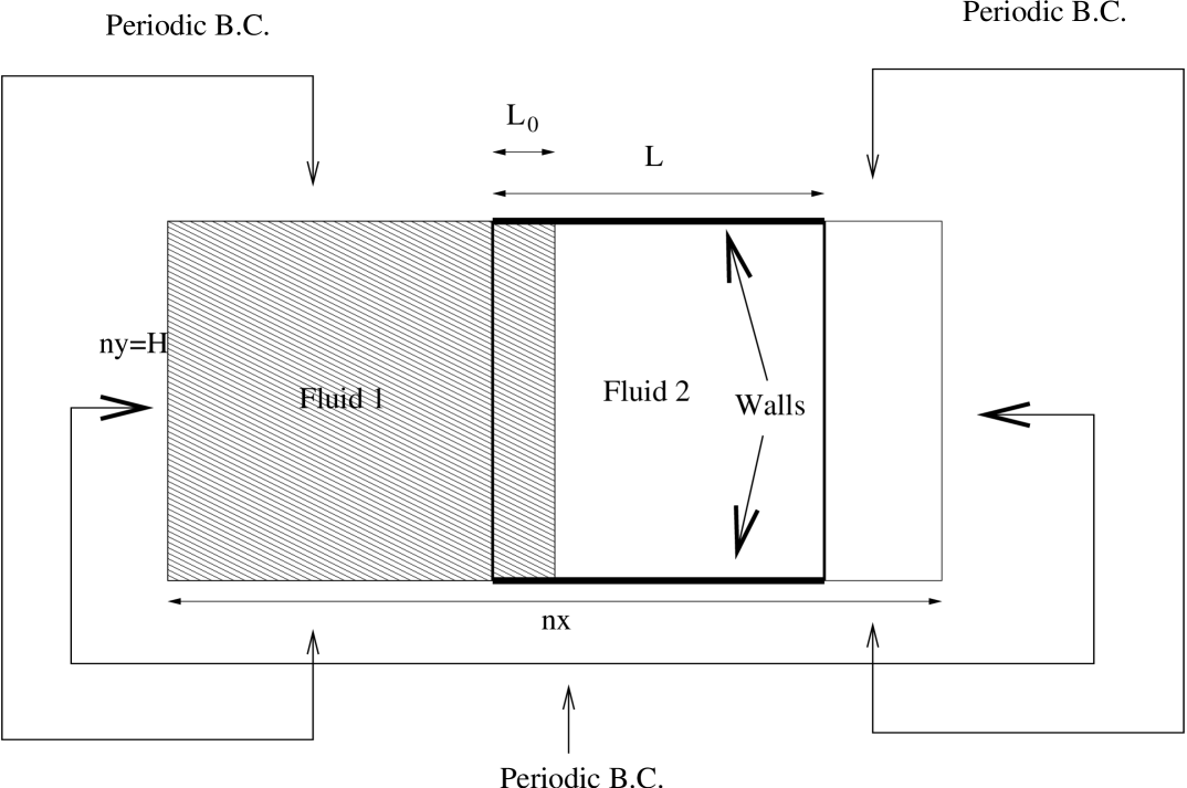
Figure 1: Geometrical set-up of the numerical LBE. The two dimensional geometry, with length $2L$ and width $H$, is divided in two parts. The left part has top and bottom periodic boundary conditions such as to support a perfectly flat gas-liquid interface, mimicking a “infinite reservoir”. In the right half, of length $L$, there is the true capillary: the top and bottom boundary conditions are those of a solid wall, with a given contact angle $\theta$. Periodic boundary conditions are also imposed at the west and east sides.

At the fluid/solid interface, the wall is regarded as a phase with constant number density. The interaction force between the fluid and wall is described as

$${\bf F}_{2k}({\bf x})=-n_{k}({\bm{x}})\sum_{{\bm{x}}^{\prime}}g_{kw}n_{w}({\bm{x}}^{\prime})({\bm{x}}^{\prime}-{\bm{x}})$$ (10)

where $n_{w}$ is the number density of the wall and $g_{kw}$ is the interaction strength between component $k$ and the wall. By adjusting $g_{kw}$ and $n_{w}$ , different wettabilities can be obtained. This approach allows the definition of a static contact angle $\theta$, by introducing a suitable value for the wall density $n_{w}$ Kan_02 , which can span the range $\theta\in[0^{o}:180^{o}]$. In particular, we have chosen $g_{1w}=0,g_{2w}=-g_{12}$ while $n_{w}$ is varied in order to adjust the wettability. In the sequel, we choose $g_{12}=0.2$ which indicates that species $2$ is attracted by the wall (hydrophilic), while species $1$ is neutral. Let us note that high values of $n_{w}$ are associated with hydrophilicity.

In a region of pure $k$th component, the pressure is given by $p_{k}=(c_{s}^{k})^{2}m_{k}n_{k}$, where $(c_{s}^{k})^{2}=\frac{3}{5}(1-\alpha_{k})$. To simulate a multiple component fluid with different densities, we let $(c_{s}^{k})^{2}m_{k}=c_{0}^{2}$, where $c_{0}^{2}=1/3$. Then, the pressure of the whole fluid is given by $p=c_{0}^{2}\sum_{k}n_{k}+\frac{3}{2}\sum_{k,\bar{k}}g_{k,\bar{k}}\Psi_{k}\Psi_{\bar{k}}$, which represents a non-ideal gas law. The viscosity is given by $\nu=\frac{1}{3}(\sum_{k}\beta_{k}\tau_{k}-\frac{1}{2})$, where $\beta_{k}$ is the mass density concentration of the $k$th component.

The Chapman-Enskog expansion wolf shows that the fluid mixture follows the Navier-Stokes equations for a single fluid:

$$\partial_{t}\rho+\nabla\cdot(\rho{\bf u}) = 0,$$ (11)

$$\rho[\partial_{t}{\bm{u}}+({\bm{u}}\cdot{\bm{\nabla}}){\bm{u}}] = -{\bf\nabla}{P}+{\bm{F}}+{\bm{\nabla}}\cdot(\nu\rho({\bm{\nabla}}{\bm{u}}+{\bm{u}}{\bm{\nabla}})$$

where $\rho=\sum_{k}\rho_{k}$ is the total density of the fluid mixture and the whole fluid velocity ${\bf u}$ is defined by $\rho{\bf u}=\sum_{k}\rho_{k}{\bf u}_{k}+\frac{1}{2}\sum_{k}{\bf F}_{k}$.

2.2 Numerical Results

All simulations were performed using the Shan-Chen model described above, setting $\nu_{l}=\nu_{g}=0.167$, $\rho_{l}=\rho_{g}=1$, $g_{12}=0.2$, $\alpha=4/9$, that is $c_{s}^{2}=\frac{1}{3}$, and the interfacial tension is $\gamma=0.07$. The channel length is chosen to be $L=450$. By taking $\theta$ constant in time, a simple analytical solution of equation (1) can be obtained:

$$z(t)=\frac{V_{cap}Hcos\theta}{6L}t_{d}\left[\exp(-t/t_{d})+t/t_{d}-1\right]+z_{0},$$ (12)

where $z_{0}$ is the starting point of the interface at the beginning of the simulation, $t_{d}=\frac{\rho H^{2}}{12\mu}$ is a typical transient time and $V_{cap}=\frac{\gamma}{\mu}$ is the capillary speed. This solution has been used to compare with simulations.

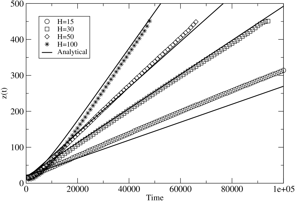
Figure 2: Front displacement vs time for different channel height $H=15,30,50,100$ with their corresponding analytical solutions. The discrepancy from washburn’s law is stronger for the smallest channel. The channel length is always $L=450$ except for H=100, for which $L=500$.

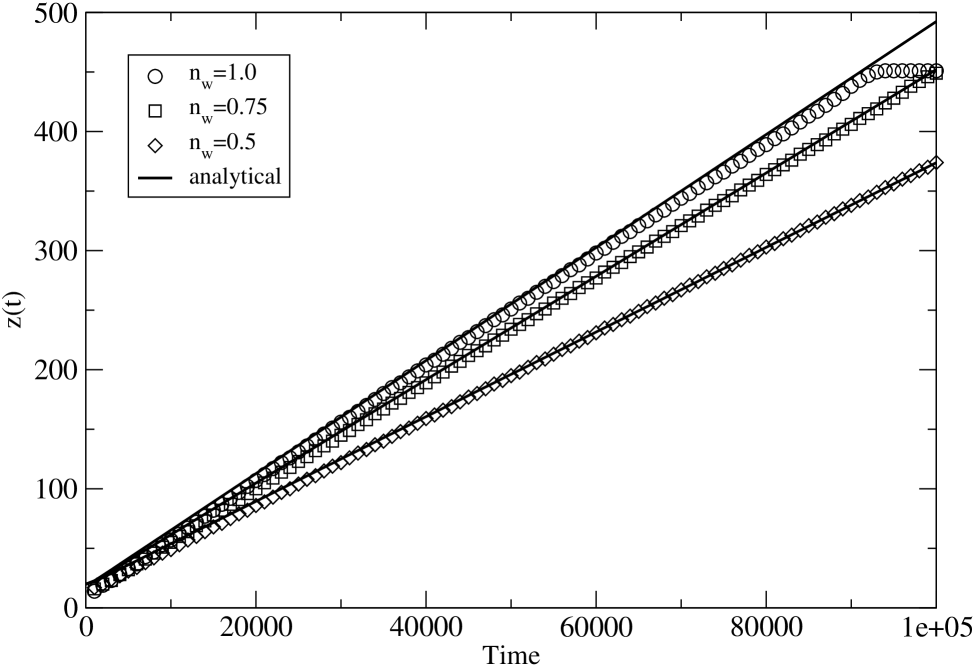
Figure 3: Front dynamics for different $n_{w}$ ($1.0,0.75,0.5$) that is for different degree of wettability. The configuration considered is with $H=30$. The case $n_{w}=0.5$ is fitted by an analytical solution with $\theta=0.78$ and the case $n_{w}=0.75$ with $\theta=0.52$.

The front displacement as a function of time is shown in Fig. 2 for different values of the channel height $H=15,30,70,100$, at $n_{w}=1$, for which static contact angle was found to be $\theta\approx 5$. As expected, the velocity of the front grows with channel height. The analytical curves are given by the solution of Eq. (12), where the contact angle is the dynamic one computed from numerical data. The contact angles computed for the four heights $15,30,50,100$ are respectively $0^{\circ},11^{\circ},25^{\circ},45^{\circ}$. The dynamic contact angle has been obtained directly as the slope of the contours of near-wall density field, and independently through the Laplace’s law, $\Delta P=\frac{2\gamma cos\theta}{H}$. The latter has been chosen for the comparison with analytical fitting curves, because the direct computation from density contours turns out to be less precise. Nevertheless, the values calculated in the two ways are approximately consistent. For instance, the contact angle computed for the case $H=30$ from the direct measurements of the pressure is $\theta\approx 12^{\circ}$ against the value $\theta\approx 11^{\circ}$ computed via density contours. Some comments on the front dynamics are in order.. The case of smallest channel height does not follow the analytical solution, showing the finite size of the interface ($w/H~{}1/3$) significantly affects the results. On the other hand, for a larger channel, good agreement between numerical and theoretical results not only holds asymptotically, but it also extents to the initial transient. This is particularly true for the largest height $H=100$, where the transient time-scale $t_{d}=\frac{\rho H^{2}}{12\mu}$ is sufficiently long to make the exponential term in the solution (12) important over a macroscopic time span. The results show that the dynamic contact angles experience a strong dependence on the channel height. In particular, in small channels, dynamic contact angles remain near their static values. On the other hand, for large ones the discrepancy is evident. This is due to the increasing value of the capillary number ($Ca\sim 0.03$ for $H=100$), since it is known that there is a correction of the dynamic contact angles due to finite capillary numbers. This correction takes the form the general form $cos(\theta_{d})-cos(\theta_{s})=g(Ca)$. Our results are best fitted by $g(Ca)=18~{}Ca^{1.2}$, which is in line with previous forms used in different LBE methods Roth_07 ; Wolf_04

Hereafter the configuration with $H=30$ and $n_{w}=1.0$ will be used as a reference for all simulations. In figure 3, the front dynamics is shown for the case $n_{w}=1.0,~{}0.75,~{}0.5$. As expected, it is found that more hydrophobic cases correspond to smaller velocities . The analytical solutions which fit the numerical data are obtained respectively with $\theta=22^{\circ},\theta=24^{\circ},\theta=40^{\circ}$. These angles are consistent with the values computed via Laplace’s law directly from numerical data, that is $\theta=0.2,~{}\theta=0.37,~{}\theta=0.69$.

Velocity profiles taken at time $t=50000$ at different positions are shown in fig. 4, for the standard case $H=30$, $n_{w}=1.0$.

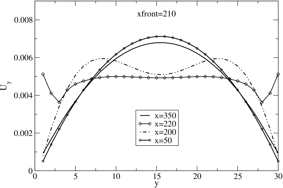
Figure 4: Velocity profile $U_{x}(y)$ for different cuts taken at time $t=40000$ with the front located at at $x\approx 210$. One cut is taken far behind the front, $x=50$, another is far ahead at $x=350$. For these cases, approximately the same Poiseuille parabolic flow is found. The other two curves correspond to the velocities just ahead and behind the interface. In these case, the velocity profile is necessarily distorted in order to let the interface advance with an uniform velocity along $y$. The interface acts as an obstacle and the velocity shows a corresponding decrease (but not a recirculation) in the middle of the channel, giving rise to a two-humped profile.

Some comments are in order. The velocity profile is parabolic everywhere except very near the interface. This is consistent with the assumption of a parabolic (Poiseuille) velocity profile. A small difference is present between the parabolic profile ahead and past the interface. This is tentatively interpreted as due to the different boundary conditions applied to the fluids ($n_{w}=1$ for the hydrophilic invading fluid 1, and $n_{w}=0$ for fluid 2 ahead of the front). This difference were found to disappear by setting nearer values of $n_{w}$ for both fluids.

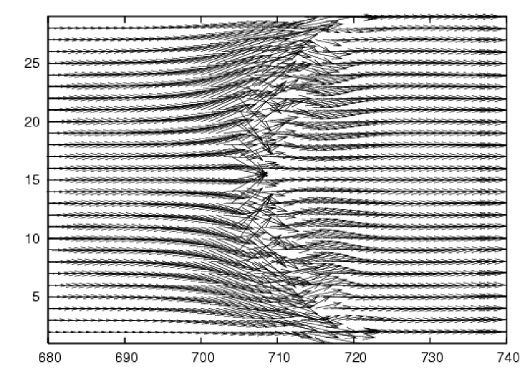
Figure 5: Velocity streamlines. The value of velocities are magnified by a factor $1000$. The interface is located at $x\approx 710$. Near the interface the profile is distorted and a secondary flow appears.

In other terms, boundary conditions are such that the fluid after the interface is less slipping, with a velocity at the wall almost recovering no-slip condition.

In fig. 5, velocity patterns are presented. Consistently with fig. 4, this figure shows that the flow is one-directional far from the interface, confirming the assumption of a Poiseuille flow. Moreover, although the flow appears to be distorted near the interface to allow slippage, no recirculation is observed at variance with other methods LBEs Fab_07 ; Wolf_04 ; Roth_07 , spurious currents are negligible. The spikes in fig. 4 reflect the existence of a hydrodynamic singularity near the wall. A detailed understanding of the LB dynamics in the near vicinity of this singularity remains an open issue for future research.

3 Conclusions

The present study shows that Lattice Boltzmann models with pseudo-potential energy interactions are capable of reproducing the basic features of capillary filling for binary fluids, as described within the Washburn approximation. Moreover, it has been shown that the method is able to reproduce the expected front dynamics for different degree of surface wettability, as well as the correct Poiseuille velocity profile, in the whole domain, except for a thin region near the interface. Quantitative agreement has been obtained with a sufficiently thin interface, $w/H<0.3$ and with two fluids at the same density. It would be desirable to extend the LB scheme in such a way to achieve larger density contrasts and interface widths of the order of the lattice spacing $\Delta x$ (current values are about $5\Delta x$). Work along these lines is underway.

4 Acknowledgments

Work performed under the EC contract NMP3-CT-2006-031980 (INFLUS) and funded by the Consorzio COMETA within the project PI2S2 (http://www.consorzio-cometa.it). Discussions with Dr. F. Toschi are kindly acknowledged.

References

- (1) E.W. Washburn, Phys. Rev. 27 (1921) 273.
- (2) R. Lucas, Kooloid-Z 23 (1918) 15.
- (3) J. Szekelely, A:W. Neumann, and Y.K. Chuang Journal of Coll. and Int. Science, 35 (1971) 273.
- (4) P.G. de Gennes, Rev. Mod. Phys. 57 (1985) 827.
- (5) L.J. Yang, T.J. Yao and Y.C. Tai, J. Micromech. Microeng. 14 (2004) 220.
- (6) N.R. Tas et al., Appl. Phys. Lett. 85 (2004) 3274.
- (7) X. Shan, and H. Chen Phys Rev E 47, 1815 (1993).
- (8) Kang, Zhang and Chen PHF 14 (9) 3203, 2002
- (9) D.A. Wolf-Gladrow Lattice-gas Cellular Automata and Lattice Boltzmann Models (Springer, Berlin, 2000).
- (10) Hou, Shan, Zou, Doolen and Soll, JCP 138(2), 1997.
- (11) M. Latva-Kokko, and D.H. Rothman Phys Rev Lett to be published.
- (12) L. Dos Santos, F. Wolf, and P. Philippi J. Stat. Phys. 121, 197 (2005).
- (13) F. Diotallevi, L. Biferale, S. Chibbaro, F. Toschi, and S. Succi EpjB submitted.