Generalization of Jeffreys’ Divergence Based Priors
for Bayesian Hypothesis testing

Abstract

In this paper we introduce objective proper prior distributions for hypothesis testing and model selection based on measures of divergence between the competing models; we call them divergence based (DB) priors. DB priors have simple forms and desirable properties, like information (finite sample) consistency; often, they are similar to other existing proposals like the intrinsic priors; moreover, in normal linear models scenarios, they exactly reproduce Jeffreys-Zellner-Siow priors. Most importantly, in challenging scenarios such as irregular models and mixture models, the DB priors are well defined and very reasonable, while alternative proposals are not. We derive approximations to the DB priors as well as MCMC and asymptotic expressions for the associated Bayes factors.

Keywords: Bayes factors; Information Consistency; Intrinsic priors; Irregular models; Kullback-Leibler divergence; Mixture models.

1 Introduction

For the data $y$, with density $f(\mbox{\boldmath{$y$}}\mid\mbox{\boldmath{$\theta$}},\mbox{\boldmath{$\nu$}})$, we consider the hypothesis testing problem:

$$H_{1}:\mbox{\boldmath{$\theta$}}=\mbox{\boldmath{$\theta$}}_{0},\hskip 7.11317pt\mbox{vs.}\hskip 7.11317ptH_{2}:\mbox{\boldmath{$\theta$}}\neq\mbox{\boldmath{$\theta$}}_{0},$$ (1)

where $\mbox{\boldmath{$\theta$}}_{0}\in\Theta$ is a known value. This is equivalent to the model selection problem of choosing between models:

$$M_{1}:f_{1}(\mbox{\boldmath{$y$}}\mid\mbox{\boldmath{$\nu$}}_{1})=f(\mbox{\boldmath{$y$}}\mid\mbox{\boldmath{$\theta$}}_{0},\mbox{\boldmath{$\nu$}}_{1})\hskip 7.11317pt\mbox{vs.}\hskip 7.11317ptM_{2}:f_{2}(\mbox{\boldmath{$y$}}\mid\mbox{\boldmath{$\theta$}},\mbox{\boldmath{$\nu$}}_{2})=f(\mbox{\boldmath{$y$}}\mid\mbox{\boldmath{$\theta$}},\mbox{\boldmath{$\nu$}}_{2}),$$ (2)

where the notation reflects the fact that often $\mbox{\boldmath{$\nu$}}_{1}$ and $\mbox{\boldmath{$\nu$}}_{2}$ represent different quantities in each model. In Jeffreys’ scenarios (Jeffreys, 1961), $\mbox{\boldmath{$\nu$}}_{1}$ and $\mbox{\boldmath{$\nu$}}_{2}$ had the same meaning; he called $\theta$ the new parameter, and $\mbox{\boldmath{$\nu$}}_{1}$ and $\mbox{\boldmath{$\nu$}}_{2}$, the common parameters (also known as nuisance parameters). We revisit this issue in Section 4.

We aim for an objective Bayes solution to this model selection problem; that is, no ‘external’ (subjective) information is assumed, other than the data, $y$, and the information implicitly needed to pose the problem, choose the competing models, etc. An excellent exposition of the advantages of Bayesian methods, specially objective Bayes methods, for problems with model uncertainty is Berger and Pericchi (2001).

Usual Bayesian solutions (for $0$-$k_{i}$ loss functions) to (1) (or, equivalently, to (2)) are based on the posterior odds:

$$\frac{\mbox{Pr}(H_{1}\mid\mbox{\boldmath{$y$}})}{\mbox{Pr}(H_{2}\mid\mbox{\boldmath{$y$}})}=\,\frac{\mbox{Pr}(H_{1})}{\mbox{Pr}(H_{2})}\ \times B_{12}\,,$$

where $\mbox{Pr}(H_{i}),\ i=1,2$ are the prior probabilities of the hypotheses, and $B_{12}$ is Bayes Factor for $H_{1}$ against $H_{2}$:

$$B_{12}=\frac{m_{1}(\mbox{\boldmath{$y$}})}{m_{2}(\mbox{\boldmath{$y$}})}=\frac{\int\,f_{1}(\mbox{\boldmath{$y$}}\mid\mbox{\boldmath{$\nu$}}_{1})\,\pi_{1}(\mbox{\boldmath{$\nu$}}_{1})\,d\mbox{\boldmath{$\nu$}}_{1}}{\int\,f_{2}(\mbox{\boldmath{$y$}}\mid\mbox{\boldmath{$\theta$}},\mbox{\boldmath{$\nu$}}_{2})\,\pi_{2}(\mbox{\boldmath{$\theta$}},\mbox{\boldmath{$\nu$}}_{2})\,d\mbox{\boldmath{$\theta$}}\,d\mbox{\boldmath{$\nu$}}_{2}}\ ,$$ (3)

where $\pi_{1}(\mbox{\boldmath{$\nu$}}_{1})$ is the prior under $H_{1}$ and $\pi_{2}(\mbox{\boldmath{$\theta$}},\mbox{\boldmath{$\nu$}})$ the prior under $H_{2}$. That is, $B_{12}$ is the ratio of the marginal (averaged) likelihoods of the models.

It is common practice in objective Bayes approaches to concentrate on derivations of the Bayes factors, letting the ultimate choice (whether objective or subjective) of the prior model probabilities (and the derivations of the posterior odds) to the user. Bayes factors were extensively used by Jeffreys (1961) as a measure of evidence in favor of a model (see also Berger, 1985; Berger and Delampady, 1987, and Berger and Sellke, 1987); Kass and Raftery (1995) is a good reference for review and applications. Bayes factors are also crucial ingredients of model averaging approaches (see Clyde, 1999; Hoeting et al, 1999). In the rest of the paper, we concentrate on the derivation of objective priors to compute Bayes factors.

A main issue for deriving objective Bayes factors is appropriate choice of $\pi_{1}(\mbox{\boldmath{$\nu$}}_{1})$ and $\pi_{2}(\mbox{\boldmath{$\theta$}},\mbox{\boldmath{$\nu$}}_{2})$ for use in (3). It is well known that familiar improper objective priors (or non-informative priors) for estimation problems (under a fixed model) are usually seriously inadequate in the presence of model uncertainty, generally producing arbitrary answers. (Interesting exceptions are studied in Berger, Pericchi and Varshavsky, 1998.) Of course, when improper priors can not be used, use of arbitrarily vague (but proper) priors is not a cure, and generally it is even worse. Another bad solution often encountered in practice is use of an apparently ‘innocuous’, harmless, but yet arbitrary, proper prior, since it can severely dominate the likelihood in ways that are not anticipated (and can not be investigated for high dimensional problems).

There are two basic approaches to compute Bayes factors when there is not enough information available for trustworthy subjective assessment of $\pi_{1}(\mbox{\boldmath{$\nu$}}_{1})$ and $\pi_{2}(\mbox{\boldmath{$\theta$}},\mbox{\boldmath{$\nu$}}_{2})$ . A very successful one is to directly derive the objective Bayes factors themselves, usually by ‘training’ and calibrating in several ways the non-appropriate Bayes factors obtained from usual objective improper priors (see Berger and Pericchi, 2001 for reviews and references). However, all these objective Bayes factors should ultimately be checked to correspond (approximately) to a genuine Bayes factor derived from a sensible prior. The alternative approach is to look for ‘formal rules’ for constructing ‘objective’ but proper priors that have nice properties and are appropriate for using in model selection; Bayes factors are then just computed from these objective proper priors. Whether these Bayes factors are appropriate can then be directly judged from the adequacy of the priors used.

Choice of prior distributions in scenarios of model uncertainty is still largely an open question, and only partial answers are known. Several methods have been proposed for use in general scenarios, like the arithmetic intrinsic (AI) priors (Berger and Pericchi, 1996; Moreno, Bertolino and Racugno, 1998); the fractional intrinsic (FI) priors (De Santis and Spezaferri, 1999; Berger and Mortera, 1999); the expected posterior (EP) priors (Pérez and Berger, 2002); the unit information priors (Kass and Wasserman, 1995) and predictively matched priors (Ibrahim and Laud, 1994; Laud and Ibrahim, 1995; Berger, Pericchi and Varshavsky, 1998; Berger and Pericchi, 2001). In the specific context of linear models, widely used prior with nice properties are Jeffreys-Zellner-Siow (JZS) priors (Jeffreys, 1961; Zellner and Siow, 1980,1984; Bayarri and García-Donato, 2007). An interesting generalization is the mixtures of $g$-priors (Liang et al., 2007).

All these methods are insightful, provide many interesting and useful ideas, and indeed have shown to behave nicely in a number of testing and model selection problems. Nonetheless, except for the very specific scenario of linear models, nobody seems to have investigated the ramifications of Jeffreys (1961) pioneering proposal (see the end of Section 2). His was indeed the first general derivation of objective priors for hypothesis testing, and was intended as a generalization of his proposal for testing a normal mean. Given the success of the generalization of this Jeffrey’s testing prior to linear models (Zellner and Siow, 1980,1984; Bayarri and García-Donato, 2007), it is somewhat surprising that his general proposal has not been pursued. We think that it is historically important to pursue this investigation, and we do so in this paper.

Specifically, we generalize Jeffrey’s pioneering suggestion, and use divergence measures between the competing models to derive the required (proper) priors. We call these priors divergence based (DB) priors. The main motivation was to generalize the useful JZS priors for use in scenarios other than the normal linear model, while at the same time extending Jeffrey’s general proposal. We will show that indeed the DB priors are the JZS priors in linear model contexts; also, they are as easy to derive (often easier) than other popular proposals (AI, FI or EP priors), being quite similar to them in many instances; most interestingly, they are well defined in certain scenarios where all of the other proposals fail.

For clarity of exposition, we consider first the case when there are no nuisance parameters. Development for the general case is delayed till Section 4, once the basic ideas have been introduced, and the behavior of DB priors studied in this considerably simpler scenario.

2 DB priors

Assume first the problem without nuisance parameters:

$$M_{1}:f_{1}(\mbox{\boldmath{$y$}})=f(\mbox{\boldmath{$y$}}\mid\mbox{\boldmath{$\theta$}}_{0})\hskip 7.11317pt\mbox{vs.}\hskip 7.11317ptM_{2}:f_{2}(\mbox{\boldmath{$y$}}\mid\mbox{\boldmath{$\theta$}})=f(\mbox{\boldmath{$y$}}\mid\mbox{\boldmath{$\theta$}}).$$ (4)

That is, the simpler model ($M_{1}$) involve no unknown parameters; hence only the prior for $\theta$ under $M_{2}$ is needed. We drop the subindex in the previous section and denote such prior simply by $\pi(\mbox{\boldmath{$\theta$}})$; clearly $\pi(\mbox{\boldmath{$\theta$}})$ has to be proper.

Our proposal for DB priors for $\theta$ will be in terms of divergence measures between the competing models $f(\mbox{\boldmath{$y$}}\mid\mbox{\boldmath{$\theta$}}_{0})$ and $f(\mbox{\boldmath{$y$}}\mid\mbox{\boldmath{$\theta$}})$, based on Kullback-Leibler directed divergences

$$KL[\mbox{\boldmath{$\theta$}}_{0}:\mbox{\boldmath{$\theta$}}]=\int[\log f(\mbox{\boldmath{$y$}}\mid\mbox{\boldmath{$\theta$}})-\log f(\mbox{\boldmath{$y$}}\mid\mbox{\boldmath{$\theta$}}_{0})]\,f(\mbox{\boldmath{$y$}}\mid\mbox{\boldmath{$\theta$}})\,d\mbox{\boldmath{$y$}},$$ (5)

(assuming continuous $y$ for simplicity). $KL$ is a measure of the information in $y$ to discriminate between $\theta$ and $\mbox{\boldmath{$\theta$}}_{0}$; it is designed to measure how far apart the two competing densities are in the sense of the likelihood (Schervish, 1995).

We do not directly use $KL$ to define the DB prior because it is not symmetric with respect to its arguments, and hence it would likely result in nonsymmetric priors; however, symmetric measures of divergence can be derived by taking sums (which was Jeffrey’s choice) or minimums of $KL$ divergences. We define:

$$D^{S}[\mbox{\boldmath{$\theta$}},\mbox{\boldmath{$\theta$}}_{0}]=KL[\mbox{\boldmath{$\theta$}}:\mbox{\boldmath{$\theta$}}_{0}]+KL[\mbox{\boldmath{$\theta$}}_{0}:\mbox{\boldmath{$\theta$}}],$$ (6)

and

$$D^{M}[\mbox{\boldmath{$\theta$}},\mbox{\boldmath{$\theta$}}_{0}]=2\times\;\min\{KL[\mbox{\boldmath{$\theta$}}:\mbox{\boldmath{$\theta$}}_{0}],KL[\mbox{\boldmath{$\theta$}}_{0}:\mbox{\boldmath{$\theta$}}]\}.$$ (7)

We multiply by $2$ the minimum in the definition of $D^{M}$ so that both measures are in the same scale; indeed, in some symmetric models (like in the normal scenario) both measures of divergence coincide. Generalizations of $KL$, $D^{S}$ and $D^{M}$ to include marginal parameters are discussed in Section 4. Note that $D^{M}$ is well defined even when one of directed $KL$ divergences is not, which is the case when the competing models have different support. Except for these irregular scenarios, $D^{S}$ is well defined and it is considerably easier to derive than $D^{M}$. Most of the derivations and properties to follow are common to both $D^{S}$ and $D^{M}$. To avoid tedious repetitions, we then simply use $D$ to refer to anyone of them. We use the superindex $S$ or $M$ only when necessary.

It is well known that $D\geq 0$ with equality if and only if $\mbox{\boldmath{$\theta$}}=\mbox{\boldmath{$\theta$}}_{0}$, although it is not a metric (the triangle inequality does not hold). Our proposal, is based on unitary measures of divergence, $\bar{D}$, which we take to be $D$ divided by the effective sample size $n^{*}$, $\bar{D}=D/n^{*}$. In simple univariate i.i.d. data the effective sample equals the number of scalar data points, but it does not need to be so in general. Indeed, in complex situations, it can be a difficult concept; although there have been several attempts in the literature to formalize it (see e.g. Pauler, 1998; Pauler, Wakefield and Kass, 1999; Berger et al. 2007), no general agreed definition seems to exist. In all of the examples of this paper, it is quite clear what $n^{*}$ should be, so we rely for now in simple, intuitive interpretations.

2.1 Motivation: scalar location parameters

Suppose $y$ is a random sample from a univariate location family:

$$f(\mbox{\boldmath{$y$}}\mid\theta)=\prod_{i=1}^{n}\,f(y_{i}\mid\theta)=\prod_{i=1}^{n}\,g(y_{i}-\theta),\hskip 7.11317pt\theta\in{\cal R}.$$

It has been argued (Berger and Delampady 1987; Berger and Sellke 1987) that in symmetric problems with $\Theta={\cal R}$, objective testing priors $\pi(\theta)$ under $H_{2}:\theta\neq\theta_{0}$ should be unimodal and symmetric about $\theta_{0}$; these priors prevent introducing excessive bias toward $H_{2}$. Accordingly, we look for a proper $\pi(\theta)$ which, when in this simple scenario, has these desirable characteristics and which is easily generalizable to other situations.

As before, let $\bar{D}$ be a unitary symmetrized divergence. We consider use of a function, $h$ of $\bar{D}$ as a testing prior under $H_{2}$; that is $\pi(\theta)\propto h(\bar{D}[\theta,\theta_{0}])$. Since $\pi$ has to be proper, $h(t)$ has to be a decreasing (no-increasing) function for $t>0$. A first possibility could be to take $h(t)=\exp\{-qt\}$ for some $q>0$, but this results in priors with short tails. Short-tailed priors are usually not adequate for model selection, since they tend to exhibit undesirable (finite sample) inconsistent behavior (see Liang et al 2007).

We explore instead use of the functions $h_{q}(t)=(1+t)^{-q}$, where $q>0$ controls thickness of the tails of $\pi(\theta)$. Let

$$c(q)=\int\,h_{q}(\bar{D}[\theta,\theta_{0}])\,d\theta=\int\,\left(1+\frac{D[\theta,\theta_{0}]}{n^{*}}\right)^{-q}\,d\theta,$$

and define

$$\underline{q}=\inf\{q\geq 0:\hskip 2.84544ptc(q)<\infty\},\hskip 19.91684ptq_{*}=\underline{q}+1/2.$$

For finite $\underline{q}$, our specific proposal for a DB prior in this location problem is

$$\pi^{D}(\theta)=c(q_{*})^{-1}\,\left(1+\frac{D[\theta,\theta_{0}]}{n^{*}}\right)^{-q_{*}}\propto h_{q_{*}}\big{(}\bar{D}[\theta,\theta_{0}]\big{)}\,.$$ (8)

Generalization to vector valued $\theta$ is trivial.

We use $q_{*}$ instead of the more natural $\underline{q}$ because $\underline{q}$ is not guaranteed to produce proper priors. Of course, if $\underline{q}$ is finite, any $q=\underline{q}+\delta$, with $\delta>0$ results in proper priors, and hence could have been used to define a DB prior. Our specific proposal, $\delta=1/2$ was chosen to reproduce the well known Jeffreys-Zellner-Siow prior in the Normal context; in general this choice results in densities with heavy tails. Moreover, we have found that in general $0<\delta<1$ is a good choice since it produces priors without moments, which in normal scenarios is needed to avoid undesirable behavior of conjugate $g$ priors (Liang et al, 2007).

The following lemma establishes the desired symmetry and unimodality of the DB prior. The proof follows easily from properties of $D$ in these location problems and is avoided.

Lemma 2.1.

Assume $\underline{q}<\infty$; then $\pi^{D}(\theta)$ is unimodal and symmetric around $\theta_{0}$.

Definition of DB priors for scale parameters is also direct. Indeed assume that $\theta$ is a scale parameter for a positive random variable $X$; then, $\xi=\log\theta$ is a location parameter for $Y=\log X$, with density $f^{*}(y\mid\xi)$. Applying the definition in (8), the DB prior for $\xi$ is:

$$\pi^{D}(\xi)\propto h_{q_{*}}(\bar{D}^{*}[\xi,\xi_{0}]),$$ (9)

where $\xi_{0}=\log(\theta_{0})$ and $\bar{D}^{*}[\xi,\xi_{0}]$ is the unitary measure of divergence between $f^{*}(\mbox{\boldmath{$y$}}\mid\xi_{0})$ and $f^{*}(\mbox{\boldmath{$y$}}\mid\xi)$. Therefore, in the original parameterization:

$$\pi^{D}(\theta)\propto h_{q_{*}}(\bar{D}^{*}[\log\theta,\log\theta_{0}])\,\frac{1}{\theta}=h_{q_{*}}(\bar{D}[\theta,\theta_{0}])\,\pi^{N}(\theta),$$ (10)

where, because of invariance of $\bar{D}$ under reparameterizations, $\bar{D}^{*}[\log\theta,\log\theta_{0}]=\bar{D}[\theta,\theta_{0}]$, and $\pi^{N}(\theta)=1/\theta$ is the non informative prior (right Haar invariant prior) for $\theta$. Definition of DB priors for general parameters, formalized in next section, will basically be a generalization of (10).

2.2 General parameters

Assume the more general problem (4) and let $\pi^{N}(\mbox{\boldmath{$\theta$}})$ be an objective (usually improper) ‘estimation’ prior (reference, invariant, Jeffreys, Uniform, … prior) for $\theta$, and let $\xi$ be a transformation such that $\pi^{N}(\mbox{\boldmath{$\xi$}})=1$ for $\mbox{\boldmath{$\xi$}}=\mbox{\boldmath{$\xi$}}(\mbox{\boldmath{$\theta$}})$. We can then derive a DB prior for $\theta$ by considering $\xi$ as a “location parameter”, applying the definition (8), and transforming back to $\theta$. This transformation was first proposed by Jeffreys (1961). Bernardo (2005) uses it with a reference prior $\pi^{N}$ for a scalar $\theta$, and notes that $\xi$ asymptotically behaves as a location parameter.

Giving $\xi$ a DB prior for location parameters results in:

$$\pi^{D}(\mbox{\boldmath{$\xi$}})\propto h_{q_{*}}(\bar{D}^{*}[\mbox{\boldmath{$\xi$}},\mbox{\boldmath{$\xi$}}_{0}]),$$ (11)

where, as before, $\bar{D}^{*}[\mbox{\boldmath{$\xi$}},\mbox{\boldmath{$\xi$}}_{0}]$ denotes ‘unit’ (symmetrized) discrepancy between $f^{*}(\mbox{\boldmath{$y$}}\mid\mbox{\boldmath{$\xi$}})$ and $f^{*}(\mbox{\boldmath{$y$}}\mid\mbox{\boldmath{$\xi$}}_{0})$, and $\mbox{\boldmath{$\xi$}}_{0}=\mbox{\boldmath{$\xi$}}(\mbox{\boldmath{$\theta$}}_{0})$. Hence, the corresponding ($DB$) prior for $\theta$ is

$$\pi^{D}(\mbox{\boldmath{$\theta$}})\propto h_{q_{*}}(\bar{D}^{*}[\mbox{\boldmath{$\xi$}}(\mbox{\boldmath{$\theta$}}),\mbox{\boldmath{$\xi$}}(\mbox{\boldmath{$\theta$}}_{0})])\ |{\cal J}_{\theta}(\mbox{\boldmath{$\theta$}})|\propto h_{q_{*}}(\bar{D}[\mbox{\boldmath{$\theta$}},\mbox{\boldmath{$\theta$}}_{0}])\ \pi^{N}(\mbox{\boldmath{$\theta$}}),$$ (12)

as long as $\pi^{N}$ is invariant under transformations; ${\cal J}(\mbox{\boldmath{$\theta$}})$ is the jacobian of the transformation. It should be noted from (12) that the explicit transformation to $\xi$ is not needed in order to derive the prior $\pi^{D}$. We can now formally define a DB prior as follows:

Definition 2.1.

(General DB priors) For the model selection problem (4), let $\bar{D}[\mbox{\boldmath{$\theta$}},\mbox{\boldmath{$\theta$}}_{0}]$ be a unitary measure of divergence between $f(\mbox{\boldmath{$y$}}\mid\mbox{\boldmath{$\theta$}})$ and $f(\mbox{\boldmath{$y$}}\mid\mbox{\boldmath{$\theta$}}_{0})$. Also let $\pi^{N}(\mbox{\boldmath{$\theta$}})$ be an objective (possibly improper) estimation prior for $\theta$ under the complex model, $M_{2}$, and $h_{q}(\cdot)$ be a decreasing function. Define:

$$\underline{q}=\inf\{q\geq 0:\hskip 7.11317ptc(q)<\infty\},\hskip 14.22636ptq_{*}=\underline{q}+1/2,$$

where $c(q)=\int\,h_{q}(\bar{D}[\mbox{\boldmath{$\theta$}},\mbox{\boldmath{$\theta$}}_{0}])\,\pi^{N}(\mbox{\boldmath{$\theta$}})d\mbox{\boldmath{$\theta$}}$. If $q_{*}<\infty$, then a divergence based prior under $M_{2}$ is defined as

$$\pi^{D}(\mbox{\boldmath{$\theta$}})=c(q_{*})^{-1}\,h_{q_{*}}(\bar{D}[\mbox{\boldmath{$\theta$}},\mbox{\boldmath{$\theta$}}_{0}])\ \pi^{N}(\mbox{\boldmath{$\theta$}}).$$ (13)

Note that, by definition, the DB priors either do not exist, or they are proper (and hence they do not involve arbitrary constants).

Specific Proposals.

Definition 2.1 is very general, in that several definitions of $\bar{D}$, $h_{q}$ and $\pi^{N}$ could be explored (as well as different choices of $0<\delta<1$ in $q_{*}=\underline{q}+\delta$). We give specific choices which, in part, are based on previous explorations and desired properties of the resulting $\pi^{D}$; however our specific choices are mainly intended to reproduce JZS priors in normal scenarios, so that our proposals for DB priors can be best contemplated as extensions of JZS priors to non-normal scenarios.

In what follows, we take $D$ to be either $D^{S}$ in (6) or $D^{M}$ in (7), and $h_{q}(t)=(1+t)^{-q}$. Since we will explore both, we need different notations:

Definition 2.2.

(Sum and Minimum DB priors) The sum DB prior $\pi^{S}$ and the minimum DB prior $\pi^{M}$ are the DB priors given in definition 2.1 with $h_{q}(t)=(1+t)^{-q}$ and $D$ being respectively $D^{S}$ (see (6)) and $D^{M}$ (see (7)). When needed, we refer to their corresponding c’s and q’s as $c_{S},\underline{q}^{S},q_{*}^{S}$, and $c_{M},\underline{q}^{M},q_{*}^{M}$, respectively.

It can easily be shown that $c_{S}(q)\leq c_{M}(q)$, so that, for regular problems (in which $\bar{D}^{S}<\infty$), $q_{*}^{M}<\infty$ implies $q_{*}^{s}<\infty$, and therefore, in these problems, existence of $\pi^{M}$ implies existence of $\pi^{S}$.

It should be noted that, although we are not explicitly assuming a specific objective prior $\pi^{N}$ in the definition of DB priors, properties of $\pi^{N}$ are inherited by the DB prior $\pi^{D}$; some properties will be crucial for sensible DB priors, and hence appropriate choice of $\pi^{N}$ becomes very important.

We now explore some appealing properties of DB priors. Since these are common to both proposals in Definition 2.2, we drop unneeded super and sub indexes and refer to the prior simply as $\pi^{D}$. This convention will be kept through the paper; distinction between $\pi^{S}$ and $\pi^{M}$ will only be done when needed.

Local behavior of DB priors.

It can be easily checked that, when $\pi^{N}(\mbox{\boldmath{$\theta$}})=1$ (as when $\theta$ is a location parameter), then the mode of $\pi^{D}$ is $\mbox{\boldmath{$\theta$}}_{0}$ (so $\pi^{D}$ is ‘centered’ at the simplest model). We can also exploit the following (well known) approximate relationship between Kullback-Leibler divergence and Fisher information (see Kullback, 1968): for $\theta$ is in a neighborhood of $\mbox{\boldmath{$\theta$}}_{0}$

$$KL[\mbox{\boldmath{$\theta$}}_{0},\mbox{\boldmath{$\theta$}}]\approx\frac{1}{2}(\mbox{\boldmath{$\theta$}}-\mbox{\boldmath{$\theta$}}_{0})^{t}\mbox{\boldmath{$J$}}(\mbox{\boldmath{$\theta$}}_{0})(\mbox{\boldmath{$\theta$}}-\mbox{\boldmath{$\theta$}}_{0}),$$

where $\mbox{\boldmath{$J$}}(\mbox{\boldmath{$\theta$}}_{0})$ is the expected Fisher information matrix evaluated at $\mbox{\boldmath{$\theta$}}_{0}$. Hence, in a neighborhood of $\mbox{\boldmath{$\theta$}}_{0}$, the DB priors approximately behave as $k$ multivariate Student distributions, centered at $\mbox{\boldmath{$\theta$}}_{0}$, and scaled by Fisher information matrix under the simpler model. That is,

$$\pi^{D}(\mbox{\boldmath{$\theta$}})\approx\mbox{St}_{k}(\mbox{\boldmath{$\theta$}}_{0},n^{*}\,\mbox{\boldmath{$J$}}(\mbox{\boldmath{$\theta$}}_{0})^{-1}/d,\,d),$$

where $d=2\underline{q}-k+1$. Moreover, by definition of $q_{*}$, $d$ above is generally close to 1, and then the DB priors would approximately be Cauchy.

As highlighted in Section 4.3.2, the approximation above exactly holds in Normal scenarios with $d=1$, and hence the DB priors reproduce precisely the proposals of Jeffreys-Zellner-Siow.

Invariance under one-to-one transformations

An important question is whether the DB priors are invariant under reparameterizations of the problem. Suppose that $\mbox{\boldmath{$\xi$}}=\mbox{\boldmath{$\xi$}}(\mbox{\boldmath{$\theta$}})$ is a one-to-one monotone mapping $\mbox{\boldmath{$\xi$}}:\Theta\rightarrow\Theta_{\xi}$. The model selection problem (4) now becomes:

$$M_{1}^{*}:f_{1}^{*}(\mbox{\boldmath{$y$}})=f^{*}(\mbox{\boldmath{$y$}}\mid\mbox{\boldmath{$\xi$}}_{0})\hskip 7.11317pt\mbox{vs.}\hskip 7.11317ptM_{2}^{*}:f_{2}^{*}(\mbox{\boldmath{$y$}}\mid\mbox{\boldmath{$\xi$}})=f^{*}(\mbox{\boldmath{$y$}}\mid\mbox{\boldmath{$\xi$}}),$$ (14)

where $f^{*}(\mbox{\boldmath{$y$}}\mid\mbox{\boldmath{$\xi$}}(\mbox{\boldmath{$\theta$}}))=f(\mbox{\boldmath{$y$}}\mid\mbox{\boldmath{$\theta$}})$ and $\mbox{\boldmath{$\xi$}}_{0}=\mbox{\boldmath{$\xi$}}(\mbox{\boldmath{$\theta$}}_{0})$. The next result shows that, if $\pi^{N}$ is invariant under the reparameterization $\mbox{\boldmath{$\xi$}}(\mbox{\boldmath{$\theta$}})$ then so are the DB priors.

Proposition 1.

Let $\pi_{\theta}^{D}(\mbox{\boldmath{$\theta$}})$ and $\pi_{\xi}^{D}(\mbox{\boldmath{$\xi$}})$ denote the DB priors for the original (4), and reparameterized (14) problems respectively. If $\pi_{\theta}^{N}(\mbox{\boldmath{$\theta$}})\propto\pi_{\xi}^{N}(\mbox{\boldmath{$\xi$}}(\mbox{\boldmath{$\theta$}}))|{\cal J}_{\xi}(\mbox{\boldmath{$\theta$}})|$, where ${\cal J}_{\xi}$ is the Jacobian of the transformation then

$$\pi_{\theta}^{D}(\mbox{\boldmath{$\theta$}})=\pi_{\xi}^{D}(\mbox{\boldmath{$\xi$}}(\mbox{\boldmath{$\theta$}}))|{\cal J}_{\xi}(\mbox{\boldmath{$\theta$}})|.$$

Proof.

See Appendix. ∎

Under the conditions of Proposition 1, Bayes factors computed from DB priors are not affected by reparameterizations. It is important to note that invariance of DB priors is a direct consequence of both the invariance of the divergence measure used and the invariance of $\pi^{N}$. Some objective priors $\pi^{N}$ invariant under reparameterizations are Jeffreys’ priors and (partially) the reference priors.

Compatibility with sufficient statistics.

DB priors are sometimes compatible with reduction of the data via sufficient statistics. This attractive property is not shared by other objective Bayesian methods, as intrinsic Bayes factors.

Proposition 2.

Let $\mbox{\boldmath{$t$}}=\mbox{\boldmath{$t$}}(\mbox{\boldmath{$y$}})$ be a sufficient statistic for $\theta$ in $f(\mbox{\boldmath{$y$}}\mid\mbox{\boldmath{$\theta$}})$ with distribution $f^{*}(\mbox{\boldmath{$t$}}\mid\mbox{\boldmath{$\theta$}})$. Assume that $\pi^{N}$ and $n^{*}$ remain the same in the problem defined by $f^{*}$, then the DB prior $\pi^{D}$ for the original problem (4) is the same as the DB prior for the reduced (by sufficienty) testing problem

$$M_{1}^{*}:f_{1}^{*}(\mbox{\boldmath{$t$}})=f^{*}(\mbox{\boldmath{$t$}}\mid\mbox{\boldmath{$\theta$}}_{0})\hskip 19.91684pt{vs.}\hskip 19.91684ptM_{2}^{*}:f_{2}^{*}(\mbox{\boldmath{$t$}}\mid\mbox{\boldmath{$\theta$}})=f^{*}(\mbox{\boldmath{$t$}}\mid\mbox{\boldmath{$\theta$}}).$$ (15)

Proof.

See Appendix. ∎

DB priors and Jeffreys’ general rule.

Jeffreys (1961) proposed objective proper priors for testing situations other than the normal mean. Specifically, when $y$ is a random sample of size $n$, and for univariate $\theta$ he proposed the following model testing prior:

$$\pi^{J}(\theta)=\frac{1}{\pi}\frac{d}{d\theta}\tan^{-1}\left(\frac{D^{S}[\theta,\theta_{0}]}{n}\right)^{1/2}=\frac{1}{\pi}\left(1+\frac{{D}^{S}[\theta,\theta_{0}]}{n}\right)^{-1}\,\frac{d}{d\theta}\left(\frac{D^{S}[\theta,\theta_{0}]}{n}\right)^{1/2}.$$ (16)

This reduces to Jeffreys Cauchy proposal when $\theta$ is a normal mean. Also, when $|\theta-\theta_{0}|$ is small, $\pi^{J}(\theta)$ can be approximated by

$$\pi^{J}(\theta)\approx\frac{1}{\pi}\big{(}1+\bar{D}^{S}[\theta,\theta_{0}]\big{)}^{-1}\,\pi^{NJ}(\theta),$$ (17)

where $\pi^{NJ}(\theta)$ is Jeffreys’ (estimation) prior (i.e. the squared root of the expected Fisher information).

Note that $\pi^{J}$ can lead to improper priors and at least in principle can not be applied for multivariate parameters. However, the approximation (17) was a main inspiration for the definition of DB priors, with clear similarities between them.

3 Comparative examples: simple null

In the spirit of Berger and Pericchi (2001) we investigate in this section the performance of DB priors in a series of situations chosen to be somehow representative of wider classes of statistical problems. We also explicitly derive well established, alternative proposals for objective priors in Bayesian hypothesis testing and compare their performance with that of DB priors. We show that in simple standard situations, DB priors produce similar results to these alternative proposals. More interestingly, in more sophisticated situations where these proposals fail (models with irregular asymptotics or improper likelihoods), the DB priors are well defined and very sensible.

We will compute and compare Bayes factors derived with DB priors, with those derived with two of the most popular general objective priors for objective Bayes model selection, namely:

1. Arithmetic intrinsic prior:

   $$\pi^{A}(\mbox{\boldmath{$\theta$}})=\pi^{N}(\mbox{\boldmath{$\theta$}})\,E^{M_{2}}_{\theta}\,(B_{12}^{N}(\mbox{\boldmath{$y$}}^{*})),$$

   where the Bayes factor $B^{N}$ is computed with the objective estimation prior $\pi^{N}$, and $\mbox{\boldmath{$y$}}^{*}$ is an imaginary sample of minimum size such that $0<m_{2}^{N}(\mbox{\boldmath{$y$}}^{*})<\infty$.

2. Fractional intrinsic prior:

   $$\pi^{F}(\mbox{\boldmath{$\theta$}})=\pi^{N}(\mbox{\boldmath{$\theta$}})\,\frac{\exp\{m\,E^{M_{2}}_{\theta}\log f(y\mid\mbox{\boldmath{$\theta$}}_{0})\}}{\int\,\exp\{m\,E^{M_{2}}_{\theta}\log f(y\mid\tilde{\mbox{\boldmath{$\theta$}}})\}\pi^{N}(\tilde{\mbox{\boldmath{$\theta$}}})d\tilde{\mbox{\boldmath{$\theta$}}}}.$$

In the iid case and asymptotically, $\pi^{A}$ produces the arithmetic intrinsic Bayes factor (Berger and Pericchi, 1996), and $\pi^{F}$ the fractional Bayes factor (O’Hagan, 1995) if the exponent of the likelihood is $b=m/n$ for a fixed $m$ (see De Santis and Spezaferri, 1999). Following the recommendation of Berger and Pericchi (2001) we take $m$ to be the size of the minimal training sample $\mbox{\boldmath{$y$}}^{*}$.

In the examples of this Section, $y$ is an iid sample of size $n$ from $f(y\mid\theta)$, and unless otherwise specified, $n^{*}=n$ ($n^{*}$ denotes effective sample size). We let $B_{12}^{S}$ denote the Bayes factor in favor of $H_{1}$ computed with $\pi^{S}$ (see Definition 2.2); $B_{12}^{M},B_{12}^{A}$ and $B_{12}^{F}$ are defined similarly.

3.1 Bounded parameter space (Example 1)

We begin with a simple example, in which data is a random sample from a Bernoulli distribution, that is

$$f(y\mid\theta)=\theta^{y}(1-\theta)^{1-y},\hskip 19.91684pty\in\{0,1\},\,\,\,\,\,\theta\in\Theta=[0,1],$$

and we want to test $M_{1}:\theta=\theta_{0}$ versus $M_{1}:\theta\neq\theta_{0}$. The usual estimation objective prior (both reference and Jeffreys) in this problem is the beta density $\pi^{N}(\theta)=Be(\theta\mid 1/2,1/2)\propto\theta^{-1/2}(1-\theta)^{-1/2}.$ In this case, since $\pi^{N}$ is proper, it would be tempting to use it as a testing prior. However, we will see that all $\pi^{S},\pi^{M},\pi^{A}$ and $\pi^{F}$ center around the null value $\theta_{0}$ whereas the estimation prior completely ignores it.

The DB prior for the sum-symmetrized divergence can be computed to be

$$\pi^{S}(\theta)\propto\Big{[}1+(\theta-\theta_{0})\log\frac{\theta(1-\theta_{0})}{\theta_{0}(1-\theta)}\Big{]}^{-1/2}\,\pi^{N}(\theta),$$

and the DB prior for the min-symmetrized divergence

$$\pi^{M}(\theta)\propto\Big{(}1+\bar{D}^{M}[\theta,\theta_{0}]\Big{)}^{-1/2}\,\pi^{N}(\theta),$$

where

$$\bar{D}^{M}[\theta,\theta_{0}] = \Big{\{}\begin{array}[]{ccc}2\,KL[\theta:\theta_{0}]&\mbox{if}&\min\{\theta_{0},1-\theta_{0}\}<\theta<\max\{\theta_{0},1-\theta_{0}\}\\ 2\,KL[\theta_{0}:\theta]&&\mbox{otherwise},\end{array}$$

and $KL[\theta:\theta_{0}]=\theta_{0}\log\frac{\theta_{0}}{\theta}+(1-\theta_{0})\log\frac{1-\theta_{0}}{1-\theta}$.

The intrinsic priors are derived in the next result. The proof is straightforward and hence it is omitted.

Lemma 3.1.

The arithmetic intrinsic prior is

$$\pi^{A}(\theta)=\Big{(}\frac{2}{\pi}\ (1-\theta_{0})(1-\theta)+\theta_{0}\theta\Big{)}\,\pi^{N}(\theta)$$

and the fractional intrinsic prior is

$$\pi^{F}(\theta)=\Big{(}\frac{\theta_{0}^{\theta}(1-\theta_{0})^{1-\theta}}{\Gamma(\theta+1/2)\Gamma(3/2-\theta)}\Big{)}\,\pi^{N}(\theta).$$

By construction, $\pi^{S}$ and $\pi^{M}$ are proper priors; $\pi^{A}$ is proper but $\pi^{F}$ is not. For instance, for $\theta_{0}=1/2$, $\pi^{F}$ integrates to 1.28 and for $\theta_{0}=3/4$, $\pi^{F}$ integrates to 1.18. This implies a small bias in the Bayes factor in favor of $M_{2}$. In Figure 1 we display $\pi^{S},\pi^{M},\pi^{A}$ and $\pi^{F}$ for $\theta_{0}=1/2$ and $\theta_{0}=3/4$. They can be seen to be very similar. When $\theta_{0}=1/2$ they are also similar to the objective estimation prior $Be(\theta\mid 1/2,1/2)$, but not for other values of $\theta_{0}$.

We also compute the Bayes factors for the four different priors, when $\theta_{0}=1/2$, for two different sample sizes, $n=10$ and $n=100$, and for different values of the MLE, $\hat{\theta}=\sum_{i=1}^{10}\,y_{i}/n$ (see Table 1). All the results are quite similar. As expected, $B_{12}^{F}$ gives the most support to $M_{2}$; $B_{12}^{A}$ gives the least. Both DB priors produce similar results, being slightly closer to $B_{12}^{A}$ than to $B_{12}^{F}$.

Finally, we consider application to real data taken from Conover (1971). Under the hypothesis of simple Mendelian inheritance, a cross between two particular plants produces, in a proportion of $\theta=3/4$ a specie called ‘giant’. To determine whether this assumption is true, Conover (1971) crossed $n=925$ pair of plants, getting $T=682$ giant plants. The Bayes factors in favor of the Mendelian inheritance hypothesis (simplest model) are also given in Table 1 for the four different priors. Again the results are very similar, the fractional intrinsic prior providing the least support to $M_{1}$.

Figure 1: In Bernoulli example: $\pi^{S}$ (Solid line), $\pi^{M}$ (Dot-dashed line), $\pi^{A}$ (Dots) and $\pi^{F}$ (Dashed line), for the case $\theta_{0}=1/2$ (left) and $\theta_{0}=3/4$ (right).

$n=10$	$\hat{\theta}$	$B_{12}^{S}$	$B_{12}^{M}$	$B_{12}^{A}$	$B_{12}^{F}$
	0.50	3.26	3.44	4.06	2.68
	0.65	2.14	2.24	2.58	1.75
	0.80	0.55	0.57	0.60	0.44
$n=100$
	0.50	9.74	10.28	12.56	8.03
	0.55	5.93	6.26	7.61	4.89
	0.60	1.33	1.40	1.68	1.09
Conover
		19.38	20.20	20.79	16.02

Table 1: Bayes factors in favor of $M_{1}$ for Bernoulli testing of $\theta_{0}=1/2$, for different values of the MLE and $n=10$, $n=100$. Also, Bayes factors for Conover data.

3.2 Scale parameter (Example 2)

We next consider another simple example of testing a scale parameter. Specifically, we consider that data come from the one parameter exponential model with mean $\mu$, that is,

$$f(y\mid\mu)=Exp\,(y\mid\frac{1}{\mu})=\frac{1}{\mu}\,\exp\{-\,\frac{y}{\mu}\},\hskip 28.45274pty>0,\ \ \mu>0,$$

and that it is desired to test $H_{1}:\mu=\mu_{0}\$ vs. $\ H_{2}:\mu\neq\mu_{0}$. Here $\pi^{N}(\mu)=\mu^{-1}$, and the DB priors are computed to be:

$$\pi^{S}(\mu)\propto\big{[}1+\frac{(\mu-\mu_{0})^{2}}{\mu\mu_{0}}\big{]}^{-1/2}\mu^{-1},\hskip 14.22636pt\pi^{M}(\mu)\propto\big{(}1+\bar{D}^{M}[\mu,\mu_{0}]\big{)}^{-3/2}\mu^{-1},$$

where

$$\bar{D}^{M}[\mu,\mu_{0}] = \Big{\{}\begin{array}[]{ccc}2\,KL[\mu_{0}:\mu]&\mbox{if}&\mu>\mu_{0}\\ 2\,KL[\mu:\mu_{0}]&\mbox{if}&\mu\leq\mu_{0},\end{array}$$

and $KL[\mu:\mu_{0}]=\log(\mu_{0}/\mu)-(\mu_{0}-\mu)/\mu_{0}$. The intrinsic priors are given in the next lemma (the proof is straightforward and is omitted):

Lemma 3.2.

The arithmetic and fractional intrinsic priors are

$$\pi^{A}(\mu)={\mu_{0}}^{-1}(1+\frac{\mu}{\mu_{0}})^{-2},\hskip 14.22636pt\pi^{F}(\mu)={\mu_{0}}^{-1}\exp\{-\frac{\mu}{\mu_{0}}\}=Exp\,\{\mu\mid\frac{1}{\mu_{0}}\}.$$

Figure 2: $\pi^{S}$ (upper left), $\pi^{M}$ (upper right), $\pi^{A}$ (lower left) and $\pi^{F}$ (lower right) for the Exponential testing of $\mu_{0}=5$.

The four priors are shown in Figure 2 when testing $\mu_{0}=5$. They all have similar shapes, although that of $\pi^{M}$ is somehow innusual; they have some interesting properties:

1. In the log scale, both $\pi^{M}$ and $\pi^{S}$ are symmetric around $\log\mu_{0}$; this is in accordance to Berger and Delampady (1987) and Berger and Sellke (1987) proposals, since $\log(\mu)$ is a location parameter.

2. All four priors are proper.

3. Neither the arithmetic intrinsic nor the DB priors have moments; the arithmetic fractional has all the moments.

4. $\pi^{M}$ has the heaviest tails, and $\pi^{F}$ the thinnest. $\pi^{S}$ has heavier tails than $\pi^{A}$

5. All four priors are ‘centered’ at the null value $\mu_{0}$; indeed, $\mu_{0}$ is the median of the DB priors and of $\pi^{A}$, and it is the mean of $\pi^{F}$.

The four Bayes factors $B_{12}$ in favour of $M_{1}:\mu=5$ appear in Table 2, for two values of $n$ ($n=10$ and $n=100$) and some few values of the MLE $\hat{\mu}=\sum_{i=1}^{n}y_{i}/n\in\{5,7.5,2.5\}$. We again find very similar results for the different priors, with $B_{12}^{S}$ and $B_{12}^{A}$ providing slightly more support to $M_{1}$ than $B_{12}^{M}$ and $B_{12}^{F}$ when data is compatible with $M_{1}$.

$n=10$	$\hat{\mu}$	$B_{12}^{S}$	$B_{12}^{M}$	$B_{12}^{A}$	$B_{12}^{F}$
	5	5.65	4.43	5.13	3.59
	7.5	2.36	2.02	2.09	1.58
	2.5	0.95	0.88	0.82	0.59
$n=100$
	5	17.28	12.81	15.98	10.89
	7.5	$14.6\times 10^{-4}$	$12.2\times 10^{-4}$	$13\times 10^{-4}$	$9.4\times 10^{-4}$
	2.5	$0.86\times 10^{-7}$	$0.83\times 10^{-7}$	$0.73\times 10^{-7}$	$0.54\times 10^{-7}$

Table 2: Bayes factors for the exponential testing with $\mu_{0}=5$ for different values of the MLE and $n=10$, $n=100$.

We next investigate a desirable property of Bayes factors which often fails when they are computed using conjugate priors (see Berger and Pericchi, 2001). It is natural to expect that, for any given sample size, $B_{12}\rightarrow 0$ as the evidence against the simpler model $M_{1}$ becomes overwhelming. When this property holds, we say that the Bayes factor is evidence consistent (or finite sample consistent). It is easy to show that, if $\bar{y}\rightarrow\infty$ then $B_{12}\rightarrow 0$ $\forall n$, no matter what prior is used to obtain the Bayes factor. The following lemma provides sufficient conditions for $B_{12}\rightarrow 0$ as $\bar{y}\rightarrow 0$.

Lemma 3.3.

Let $B_{12}^{\pi}$ be the Bayes factor computed with $\pi(\mu)$. $B_{12}^{\pi}\rightarrow 0$ as $\bar{y}\rightarrow 0$, for all $n\geq k>0$ if and only if

$$\int_{0}^{1}\mu^{-k}\,\pi(\mu)\,d\mu=\infty.$$ (20)

Proof.

See Appendix.∎

It follows that all four priors considered produce evidence consistent Bayes factors for all $n\geq 1$. Evidence consistency provides further insight into the behaviour of the DB priors. Indeed, we recall that in the general definition of DB priors we used the power $\underline{q}+\delta$, and then we recommended the specific choice $\delta=.5$ . Interestingly, if $\delta>1$ is used instead, then $\pi^{S}$ would not be evidence consistent as $\bar{y}\rightarrow 0$.

Last, we study the behavior of $B_{12}$ as the evidence in favor of $M_{1}$ grows (that is, as $\bar{y}\rightarrow\mu_{0}$). For this example, it is easy to show that, when $\bar{y}\rightarrow\mu_{0}$, $B_{12}$ grows to a constant, $B_{12}^{0}(n,\pi)$ say, that depends only on $n$ and the prior used. Of course, it then follows from the dominated convergence theorem that $B_{12}^{0}(n,\pi)\rightarrow\infty$ with $n$, but this also follows from general consistency of Bayes factors (for proper, fix priors), so it is not very interesting. Of more interest for our comparison is to study how fast $B_{12}^{0}(n,\pi_{2})$ goes to $\infty$. In Figure 3 we show $B_{12}^{0}(n,\pi)$ for the four priors considered. It can be seen that $\pi^{S}$ is the one producing the largest values of $B_{12}^{0}$ for all values of $n$, with those for $\pi^{A}$ following very closely.

Figure 3: Upper bounds $B_{12}^{0}(n,\pi)$ of Bayes factors as a function of $n$ for the priors $\pi^{S}$ (Solid line), $\pi^{M}$ (Dot-dashed line), $\pi^{F}$ (Dashed Line), and $\pi^{A}$ (Dots).

3.3 Location-scale (Example 3)

DB priors are defined in general for vector parameters $\theta$. As an illustration, we next consider a most popular example, namely the normal distribution; here the 2-dimensional $\theta$ has two components of different nature (location and scale). Specifically, assume that

$$f(y\mid\mu,\sigma)=N(y\mid\mu,\sigma^{2}),$$

and that we want to test $M_{1}:(\mu,\sigma)=(\mu_{0},\sigma_{0})$ versus $M_{2}:(\mu,\sigma)\neq(\mu_{0},\sigma_{0})$. This hypothesis testing problem occurs often in statistical process control, where a production process is considered ‘in control’ if its production outputs have a specified mean and standard deviation (the so called nominal values); the question of interest is whether the process is in control, that is, whether the mean and variance are equal to the nominal values.

To compute the DB priors we use the reference prior $\pi^{N}(\mu,\sigma)=\sigma^{-1}$; for the sum-DB prior we get:

$$\pi^{S}(\mu,\sigma)=\pi^{S}(\sigma)\,\pi^{S}(\mu\mid\sigma),\hskip 14.22636pt\pi^{S}(\sigma)\propto\frac{\sigma}{(\sigma_{0}^{4}+\sigma^{4})^{1/2}(\sigma_{0}^{2}+\sigma^{2})^{1/2}},$$

and

$$\pi^{S}(\mu\mid\sigma)=\mbox{Ca}(\mu\mid\mu_{0},\Sigma),\hskip 28.45274pt\Sigma=\frac{\sigma_{0}^{4}+\sigma^{4}}{\sigma_{0}^{2}+\sigma^{2}},$$

where $Ca$ represents the Cauchy density. In this example, the minimum-DB prior $\pi^{M}$ does not exist, since $\underline{q}^{M}=\infty$. It can be checked that $\pi^{S}(\mu\mid\sigma)$ is symmetric around $\mu_{0}$, which is a location parameter in $\pi^{S}(\mu\mid\sigma)$; $\sigma_{0}$ is a scale parameter in $\pi^{S}(\sigma)$. The joint density $\pi^{S}$ is shown in Figure 4.

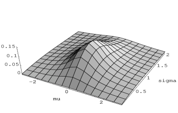
Figure 4: $\pi^{S}$ for the Normal problem, with $\mu_{0}=0,\sigma_{0}=1$.

The intrinsic priors, which have simpler forms and thinner tails, are derived next (the proof is omitted):

Lemma 3.4.

The arithmetic intrinsic prior is

$$\pi^{A}(\mu,\sigma)=\pi^{A}(\sigma)\,\pi^{A}(\mu\mid\sigma),\hskip 14.22636pt\pi^{A}(\sigma)=\frac{2}{\pi}\frac{\sigma_{0}}{\sigma^{2}+\sigma_{0}^{2}},\hskip 14.22636pt\pi^{A}(\mu\mid\sigma)=N(\mu\mid\mu_{0},\frac{\sigma^{2}+\sigma_{0}^{2}}{2}),$$

and the fractional intrinsic prior is

$$\pi^{F}(\mu,\sigma)=N^{+}(\sigma\mid 0,\frac{\sigma_{0}^{2}}{2})\ N(\mu\mid\mu_{0},\frac{\sigma_{0}^{2}}{2}),$$

where $N^{+}$ stands for the normal density truncated to the positive real line.

The intrinsic priors are proper; also, as with the sum-DB prior, $\mu_{0}$ and $\sigma_{0}$ are location and scale parameters for $\mu\mid\sigma$ and $\sigma$ respectively. Under the fractional intrinsic prior $\pi^{F}$, $\mu$ and $\sigma$ are independent a priori.

Values of $B_{12}$ for all three priors and different values of the sufficient statistic ($\bar{y}$, $S$) are given in Table 3 when $(\mu_{0},\sigma_{0})=(0,1)$. The Bayes factors corresponding to the different priors can be seen to be quite similar, specially, once again, $B_{12}^{S}$ and $B_{12}^{A}$.

For the three priors, we display in Figure 5 the marginal distributions of $\sigma$ and in Figure 6, the conditional distributions of $\mu$ given $\sigma$. It can clearly be seen that $\pi^{F}(\sigma)$ has thinner tails than $\pi_{2}^{A}$ and $\pi_{2}^{S}$ (recall, thicker tails seem to perform better for testing). Also, all conditional priors for $\mu$ are symmetric around their mode $\mu_{0}$, with $\pi^{S}(\mu\mid\sigma)$ having the heaviest tails.

	$\bar{y}=0$			$\bar{y}=1$			$\bar{y}=2$
	$B_{12}^{s}$	$B_{12}^{A}$	$B_{12}^{F}$	$B_{12}^{s}$	$B_{12}^{A}$	$B_{12}^{F}$	$B_{12}^{s}$	$B_{12}^{A}$	$B_{12}^{F}$
$S=0.5$	2.30	1.35	0.70	0.03	0.02	0.01	$3\cdot 10^{-8}$	$4\cdot 10^{-8}$	$6\cdot 10^{-8}$
$S=1$	18.67	18.55	11.72	0.21	0.19	0.18	$1\cdot 10^{-7}$	$2\cdot 10^{-7}$	$6\cdot 10^{-7}$
$S=2$	0.006	0.006	0.017	$5\cdot 10^{-5}$	$5\cdot 10^{-5}$	$21\cdot 10^{-5}$	$2\cdot 10^{-11}$	$2\cdot 10^{-11}$	$41\cdot 10^{-11}$

Table 3: For multidimensional parameter problem $(\mu_{0}=0,\sigma_{0}=1)$, values of $B_{12}$ for different values of ($\bar{y},S$) with $n=10$.

Figure 5: Marginal distributions of $\sigma$ when $(\mu_{0},\sigma_{0})=(0,1)$; $\pi_{2}^{S}(\sigma)$ (solid line), $\pi_{2}^{A}(\sigma)$ (dots), and $\pi_{2}^{F}(\sigma)$ (dashed line). The pair (mode,median) for these priors are (0.81,1.56) for $\pi^{D}$, (0,1) for $\pi^{A}$, and (0,0.48) for $\pi^{F}$.

Figure 6: Conditional distributions of $\mu$ given $\sigma=1$ (left) and $\sigma=3$ (right) when $(\mu_{0},\sigma_{0})=(0,1)$; $\pi^{S}$ (solid), $\pi^{A}$ (dots), and $\pi^{F}$ (dashed).

With respect to the evidence consistency of the Bayes factors, it is easy to show that when either $\bar{y}\rightarrow\infty$, $\bar{y}\rightarrow-\infty$ or $S\rightarrow\infty$ (the evidence against $M_{1}$ is very strong), then $B_{12}\rightarrow 0$, $\forall n$ and for the three priors considered. When the evidence in favor of $M_{1}$ is largest (that is, $(\bar{y},S)\rightarrow(\mu_{0},\sigma_{0})$) it can be seen (with a change of variables) that the Bayes factor in favor of $M_{1}$, grows to $B_{12}^{1}(n,\pi)$

$$B_{12}^{1}(n,\pi)=\int\beta^{-n}\exp\{-n\,\frac{1+\beta^{2}(\alpha^{2}-1)}{2\beta^{2}}\}\,\pi_{*}^{j}(\alpha,\beta),$$

a function only of $n$ and the prior ($j=A,F,S$) used. For the arithmetic intrinsic prior and fractional priors, the mixing densities $\pi_{*}^{j}$ are:

$$\pi_{*}^{A}(\alpha,\beta)=\frac{2\beta}{\pi^{3/2}(1+\beta^{2})^{3/2}}\exp\{-\frac{\alpha^{2}\beta^{2}}{1+\beta^{2}}\},\hskip 14.22636pt\pi_{*}^{F}(\alpha,\beta)=\frac{2\beta}{\pi}\exp\{-\beta^{2}(1+\alpha^{2})\},$$

and for the sum DB prior:

$$\pi_{*}^{S}(\alpha,\beta)=\frac{\beta^{2}}{\pi\kappa}\big{(}1+\beta^{4}+\beta^{2}\alpha^{2}(1+\beta^{2})\big{)}^{-1},\hskip 14.22636pt\kappa=\int s((1+s^{4})(1+s^{2}))^{-1/2}\,ds.$$

Figure 7 illustrates the rate at which $B_{12}^{1}(n,\pi)\rightarrow\infty$ as $n\rightarrow\infty$. It can be clearly seen that, as in the previous example, DB and intrinsic prior behave very similarly, being more sensitive to the evidence in favor $M_{1}$ than the fractional prior, subtantially so unless $n$ is very small.

Figure 7: Upper bounds $B_{12}^{1}(n,\pi)$ of Bayes factors as a function of $n$ for the priors $\pi^{S}$ (Solid line), $\pi^{M}$ (Dot-dashed line), $\pi^{F}$ (Dashed Line), and $\pi^{A}$ (Dots).

Finally we compare the behavior of the three priors in a real example taken from Montgomery (2001). The example refers to controlling the piston ring for an automotive engine production process. The process was considered to be in control if the mean and the standard deviation of the inside diameter (in millimeters) of the pistons were $\mu_{0}=74.001$ and $\sigma_{0}=0.0099$. At some specific time, the following sample was taken from the process:

$$74.035,74.010,74.012,74.015,74.026\,,$$

and it had to be checked whether the process was in control. Bayes factors are given in Table 4. $B_{12}^{F}$ provides about twice more support to $M_{1}$ than $B_{12}^{S}$ and $B_{12}^{A}$, which are very similar to each other.

$B_{12}^{S}$	$B_{12}^{A}$	$B_{12}^{F}$
0.004	0.005	0.011

Table 4: Bayes factors $B_{12}$ for Montgomery (2001) example.

3.4 Irregular models (Example 4)

There is an important class of models for which the parameter space is constrained by the data. These models do not have regular asymptotics and hence solutions based on asymptotic theory (like the Bayesian information criteria, BIC) do not apply. Moreover, these models are very challenging for the intrinsic approach; indeed, as discussed in Berger and Pericchi (2001), the fractional Bayes factor is completely unreasonable (and hence the fractional intrinsic prior is useless), and the arithmetic intrinsic prior (which was only derived for the one side problem) is “something of a conjecture” (authors’ verbatim). We take here the simplest such models, namely an exponential distribution with unknown location. Accordingly, assume that

$$f(y\mid\theta)=\exp\{-(y-\theta)\},\hskip 28.45274pty>\theta,$$

and that it is wanted to test $H_{1}:\theta=\theta_{0}$ vs. $H_{2}:\theta\neq\theta_{0}$. To the best of our knowledge, no objective priors have been proposed for this testing problem in the literature.

In these situations, the sum-symmetrized kulback-Leibler divergence $D^{S}[\theta,\theta_{0}]$ is $\infty$, so we have to use the minimum. It can be checked that $\bar{D}^{M}[\theta,\theta_{0}]=2|\theta-\theta_{0}|$, a well defined divergence. Also, $\pi^{N}(\theta)=1$ since $\theta$ is a location parameter. The Minimum DB prior is then given by

$$\pi^{M}(\theta)=\frac{1}{2}\big{(}1+2|\theta-\theta_{0}|\big{)}^{-3/2},\hskip 28.45274pt\theta\in{\cal R},$$

which is symmetric with respect to $\theta_{0}$ (as expected, since $\theta$ is a location parameter); also, $\pi^{M}$ has no moments. Figure 8 (left) shows $\pi^{M}(\theta)$ when $\theta_{0}=0$.

We next investigate the evidence consistency for any $n$. The sufficient statistic is $T=\min\{y_{1},\ldots,y_{n}\}$. It is trivially true that $B_{12}\rightarrow 0$, as $T\rightarrow-\infty$ for any (proper) prior (in fact, $B_{12}=0$ for $T<\theta_{0}$). The next lemma provides a sufficient condition on the prior to produce evidence consistency $\forall n$, as $T\rightarrow\infty$.

Lemma 3.5.

Let $\pi(\theta)$ be any proper prior (on $M_{2}$) and $B_{12}^{\pi}$ be the corresponding Bayes factor. If for some integer $k>0$

$$\int_{\theta_{0}}^{\infty}e^{k\theta}\,\pi(\theta)\,d\theta=\infty,$$ (21)

then $B_{12}^{\pi}\rightarrow 0$ as $T\rightarrow\infty$ $\forall n\geq k$.

Proof.

See Appendix.∎

It follows from the previous lemma that $\pi^{M}$ produces evidence consistent Bayes factors $\forall n\geq 1$. We next investigate the situation for increasing evidence in favor of $M_{1}$, that is, as $T\rightarrow\theta_{0}^{+}$. Let

Figure 8: Irregular example, two-side testing of $M_{1}:\theta=0$. Left: the DB prior $\pi^{M}$; Right: $B_{12}^{0}(n)$ as a function of $n$.

$$B_{12}^{0}(n)=\lim_{T\rightarrow\theta_{0}^{+}}\,B_{12}^{\pi^{D}}.$$

$B_{12}^{0}(n)$ is an upper bound of $B_{12}$ when the evidence in favor of $M_{1}$ is largest. It can be seen in Figure 8 (right) that $B_{12}^{0}(n)$ is nearly linear. Of course $B_{12}^{0}(n)\rightarrow\infty$ when $n\rightarrow\infty$.

As mentioned before, there does not seem to be any other proposals in the literature for the two-side testing problem. However, Berger and Pericchi (2001), do consider the ‘one side testing’ version, namely testing $M_{1}:\theta=\theta_{0}$ vs $M_{2}:\theta>\theta_{0}$; they conjecture that the arithmetic intrinsic prior for this problem is the proper density

$$\pi_{2}^{A}(\theta)=\big{(}-e^{\theta-\theta_{0}}\,\log(1-e^{\theta_{0}-\theta})-1\big{)},\hskip 14.22636pt\theta>\theta_{0},$$

which is a decreasing and unbounded function of $\theta$. Also, since We next compare the (minimum) DB prior for this problem with Berger and Pericchi proposal.

Although our original formulation appears to be in terms of two side testing (see (1)) in reality it suffices to define $\Theta$ appropriately to cover other testing situations. For instance, in our one-side testing, we take $\Theta=[\theta_{0},\infty)$. The (minimum) DB prior is

$$\pi^{M}(\theta)=\big{(}1+2(\theta-\theta_{0})\big{)}^{-3/2},\hskip 14.22636pt\theta>\theta_{0}.$$

It can be checked, that $\pi^{A}$ meets condition (21) for $k=1$ and hence $\pi^{A}$ produces evidence consistent Bayes factors $\forall n\geq 1$. The priors $\pi^{A}$ and $\pi^{M}$ are displayed in Figure 9. We find that also in this example $\pi^{M}$ has thicker tails.

In this one side testing scenario (in sharp contrast to the behavior in the two-side testing) the Bayes factor in favor of $M_{1}$ for every $n>0$ does grow to $\infty$ as the evidence in favor of $M_{1}$ grows. Indeed, the Bayes factor $B_{12}$ is

$$\Big{(}\int_{\theta_{0}}^{T}\,\exp\{n(\theta-\theta_{0})\}\,\pi(\theta)d\theta\Big{)}^{-1},$$

so that, $B_{12}\rightarrow\infty$ when $T\rightarrow\theta_{0}^{+}\ ,\forall n>0$, no matter what prior is used. Note that here $\theta_{0}$ is in the boundary of the parameter space.

Figure 9: Irregular, one side testing problem: $\pi^{D}$ (solid) and $\pi^{A}$ (dots) for the case $\theta_{0}=0$.

In Table 5, we produce the Bayes factors computed with $\pi^{A}$ and $\pi^{M}$ when $\theta_{0}=0$ for various values of $T=\min\{y_{1},\ldots,y_{n}\}$, and for $n=10$ and $n=20$. For small values of $T$ ($T<0.20$), when evidence supports $M_{1}$, $B_{12}^{M}$ is considerably larger than $B_{12}^{A}$, thus giving more support to $M_{1}$. For larger values of $T$ (that is, when data contradict $M_{1}$) both priors result in very similar Bayes factors.

	$T$
	0.02	0.05	0.10	0.20	0.50	1.00
	$n=10$
$B_{12}^{M}$	46.56	16.66	6.83	2.19	0.16	0.002
$B_{12}^{A}$	11.54	5.16	2.57	1.02	0.10	0.001
	$n=20$
$B_{12}^{M}$	41.96	12.65	3.75	0.55	0.002	$2\cdot 10^{-7}$
$B_{12}^{A}$	10.52	4.04	1.50	0.28	0.002	$2\cdot 10^{-7}$

Table 5: Irregular models, one side testing. Values of $B_{12}$ for different values of $T$, $n$ and for the two priors $\pi^{A},\pi^{M}$, when testing $\theta_{0}=0$.

3.5 Mixture models (Example 5)

Mixture models are among the most challenging scenarios for objective Bayesian methodology. These models have improper likelihoods, i.e., likelihoods for which no improper prior yields a finite marginal density (integrated likelihood). Recently, Pérez and Berger (2001), have used expected posterior priors (see Pérez and Berger, 2002) to derive objective estimation priors, but basically no general method seems to exist for deriving objective priors for testing with these models.

However, the divergence measures are well defined (although the integrals are now more involved) providing a reasonable DB prior to be used in model selection. We consider a simple illustration. Assume

$$f(y\mid\mu,p)=p\,N(y\mid 0,1)+(1-p)\,N(y\mid\mu,1),$$

and the testing of $H_{1}:\mu=0$, vs. $H_{2}:\mu\neq 0$, where $p<1$ is known (if $p=1$, both hypotheses define the same model). As Berger and Pericchi (2001) point out, there is no minimal training sample for this problem and hence the intrinsic Bayes factor cannot be defined. The fractional Bayes factor does not exist either. The only prior we know for this problem is the recommendation in Berger and Pericchi (2001) of using $\pi^{BP}(\mu)=Ca(\mu|0,1)$.

Although there is no formal $\pi^{N}(\mu)$ here, $\pi^{N}(\mu)=1$ is usually assumed (see for instance Pérez and Berger, 2002). It can be shown that $\underline{q}^{M}=\infty$, and hence, $\pi^{M}$ does not exist. Let

$$G(p,\mu,\mu^{*})=\int_{-\infty}^{\infty}\,\log\Big{[}1+\frac{1-p}{p}\,e^{y\mu-\mu^{2}/2}\Big{]}N(y\mid\mu^{*},1)\,dy.$$ (22)

Then

$$D^{S}[\mu,\mu_{0}]=n(1-p)\big{(}G(p,\mu,\mu)-\,G(p,\mu,0)\big{)}.$$

It can be shown that $\underline{q}^{S}<\infty$, and hence that the sum DB prior $\pi^{S}$ exists. The normalizing constant, however, can not be derived in closed form. Numerical procedures could be used to exactly derive the sum-DB prior. We use instead a Laplace approximation (see Tanner 1996) to (22) to get and approximate DB prior. Specifically

$$G(p,\mu,\mu^{*})\approx\log\Big{[}1+\frac{1-p}{p}\,e^{\mu^{*}\mu-\mu^{2}/2}\Big{]}=G^{L}(p,\mu,\mu^{*}).$$ (23)

Figure 10 shows $G(p,\mu,\mu^{*})-G(p,\mu,0)$ and its approximation $G^{L}(p,\mu,\mu^{*})-G^{L}(p,\mu,0)$ for $p=.5$ and $p=.75$. The approximation is very good as long as $p$ is not too extreme.

Figure 10: $G(p,\mu,\mu)-G(p,\mu,0)$ (solid) and its Laplace approximation $G^{L}(p,\mu,\mu)-G^{L}(p,\mu,0)$ (dots). Left: $p=0.50$. Right: $p=0.75$.

We can now use this approximation to derive the DB prior. Note that the natural effective sample size here is $n^{*}=n(1-p)$, so that the unitary sum-symmetrized divergence is

$$\bar{D}^{S}[\mu,\mu_{0}]=\frac{D^{S}(\mu,\mu_{0})}{n(1-p)}\approx\log\frac{1+\frac{1-p}{p}\ e^{\mu^{2}/2}}{1+\frac{1-p}{p}\ e^{-\mu^{2}/2}}=\bar{D}^{SL}[\mu,\mu_{0}].$$

This approximation is specially appealing because it also keeps essential properties of the divergence measures. In particular, $\bar{D}^{SL}(\mu,\mu_{0})\geq\bar{D}^{SL}(\mu_{0},\mu_{0})=0$, so that the approximate DB prior

$$\pi^{SL}(\mu)\propto\big{(}1+\bar{D}^{SL}(\mu,\mu_{0})\big{)}^{-q_{*}^{s}},$$

has a mode at zero. Since $\underline{q}^{s}=1/2$, we finally get

$$\pi^{SL}(\mu)\propto\big{(}1+\bar{D}^{LS}(\mu,\mu_{0})\big{)}^{-1}.$$

Figure 11: $\pi^{SL}$ (solid line), $Ca(0,1/1-p)$ (dashed line) and $\pi^{BP}(\mu)=Ca(\mu|0,1)$ (dots) for $p=0.50$ (left), $p=0.75$ (middle) and $p=0.25$ (right).

Interestingly, the prior $\pi^{SL}$ is close to a Cauchy density, which was Berger and Pericchi proposal, although the scale differs. Indeed a Taylor expansion of order 3, around $\mu=0$ gives

$$\bar{D}^{SL}(\mu,\mu_{0})\approx(1-p)\mu^{2},$$ (24)

so that, unless $p$ is very close to 1, $\pi^{SL}$ behaves around $0$ as a $Ca(\mu\mid 0,1/(1-p))$; the approximation is excellent when $p$ is close to 0.5. In the tails, on the other hand, we have that, as $|\mu|\rightarrow\infty$

$$\bar{D}^{SL}(\mu,\mu_{0})\approx\frac{\mu^{2}}{2},$$ (25)

independently of $p$. Hence, the tails of $\pi^{SL}$ are close to those of a $Ca(\mu\mid 0,2)$ density. Note that both approximations (24) and (25) coincide for $p=0.5$.

The scale of the $Ca(\mu\mid 0,1/(1-p))$ makes intuitive sense. Indeed, the larger $p$, the less observations providing information about $\mu$ we get, and the DB prior adjust to a less informative likelihood by inflating its scale. Figure 11 displays $\pi^{SL}$, its $Ca(\mu\mid 0,1/(1-p))$ approximation, and the proposal of Berger and Pericchi (2001) for different values of $p$. Notice that, for values of $p$ close to 0, $\pi^{SL}$ (and its approximation $Ca(0,1/1-p)$) approximately behaves as a $Ca(0,1)$, the Berger and Pericchi proposal (see Figure 11, right). This has an interesting interpretation since, as $p\rightarrow 0$ the testing problem in this example essentially coincides with that of testing $H_{1}:\mu=0$ vs. $H_{2}:\mu\neq 0$, when $\mu$ is the mean of a normal density, for which the $Ca(\mu\mid 0,1)$ is perhaps the most popular prior to be used as prior distribution for $\mu$ under $H_{2}$.

In this example, the DB prior (as well as Berger and Pericchi proposal) again produces evidence consistent Bayes factors for all $n$. Indeed, it can be shown that if one of the $y_{i}^{\prime}s$ tends to $\infty$ or $-\infty$, then the corresponding Bayes factor tends to 0 no matter what prior is used. On the other hand, as the evidence for $H_{1}$ increases, we get a finite upper bound on $B_{12}$ for every fixed sample size $n$:

$$B_{12}^{0}(n,p,\pi)=\lim_{y_{i}\rightarrow 0,\forall i}\,B_{12}.$$

In Figure 12 we show $B_{12}^{0}$ for $\pi=\pi^{SL}$ and $\pi=Ca(\mu\mid 0,1)$ as a function of $n$ for $p=0.5$. As in the previous examples, it is an immediate consequence that $B_{12}^{0}(n,p,\pi)\rightarrow\infty$ as $n\rightarrow\infty$ for both priors, but the support for $H_{1}$ is larger when $\pi^{SL}$ is used for every $n$.

Figure 12: $B_{12}^{0}$ for $\pi^{SL}$ (solid line) and $\pi^{BP}$ (dots) as a function of $n$, for $p=0.5$.

In Table 6 we show the Bayes factors $B_{12}^{SL}$, $B_{12}^{ap}$ and $B_{12}^{BP}$ computed respectively with the priors $\pi^{SL}$, its $Ca(\mu\mid 0,1/(1-p))$ approximation and the $Ca(\mu\mid 0,1)$ proposed by Berger and Pericchi. Since reduction by sufficient statistic is not possible, the Bayes factors are computed for simulated samples of size $n=20$, with mean $\mu\in\{0,0.5,1\}$, and $p\in\{0.25,.5,0.75\}$. $B_{12}^{SL}$ and its approximation $B_{12}^{ap}$ are very close, demonstrating that the approximation is very good for the considered range of $p$. $B_{12}^{SL}$ and $B_{12}^{BP}$ are also very similar.

	$p=0.25$			$p=0.5$			$p=0.75$
$\mu$	$B_{12}^{SL}$	$B_{12}^{ap}$	$B_{12}^{BP}$	$B_{12}^{SL}$	$B_{12}^{ap}$	$B_{12}^{BP}$	$B_{12}^{SL}$	$B_{12}^{ap}$	$B_{12}^{BP}$
0	5.49	4.97	4.39	2.56	2.56	2.01	2.37	2.90	1.87
0.5	1.82	1.65	1.49	0.36	0.36	0.33	1.69	2.06	1.42
1	0.07	0.06	0.06	0.04	0.04	0.04	0.01	0.01	0.01

Table 6: Bayes factors $B_{12}$ for simulated samples of size $n=20$ from the mixture model with various values of $p$ and $\mu$ and the priors $\pi^{SL}$ , its approximation $Ca(\mu\mid 0,1/(1-p))$ and $\pi^{BP}(\mu)=Ca(\mu\mid 0,1)$.

4 Nuisance parameters

In this section we deal with more realistic problems in which the distribution of the data is not fully specified under the null (simplest model), but depends on some nuisance parameter. Assume that $y_{i},\ i=1,\ldots,n$ are independent (not necessarily i.i.d.) and that $\mbox{\boldmath{$y$}}=(y_{1},\ldots,y_{n})\sim\{f(\mbox{\boldmath{$y$}}\mid\mbox{\boldmath{$\theta$}},\mbox{\boldmath{$\nu$}}),\ \mbox{\boldmath{$\theta$}}\in\Theta,\,\mbox{\boldmath{$\nu$}}\in\Upsilon\}$. We want to test $H_{1}:\mbox{\boldmath{$\theta$}}=\mbox{\boldmath{$\theta$}}_{0}$ vs. $H_{2}:\mbox{\boldmath{$\theta$}}\neq\mbox{\boldmath{$\theta$}}_{0}$. Equivalently we want to solve the model selection problem (2) where it is carefully acknowledged that $\nu$ can have a different meanings in each model.

However, from now on we assume, after suitable reparameterization if needed, that $\theta$ and $\nu$ are orthogonal (that is, that Fisher information matrix is block diagonal). It is then customary to assume that $\nu$ has the same meaning under both models (see Berger and Pericchi, 1996, for an asymptotic justification). This will be needed for the divergence measures to have intuitive meaning, and also to justify assessment of the same (possibly improper) prior for $\nu$ under both models thus considerably simplifying the assessment task. The suitability of orthogonal parameters in the presence of model uncertainty was first exploited by Jeffreys (1961) and it has been successfully used by many others (see for example Zellner and Siow, 1980, 1984, and Clyde, DeSimone and Parmigiani, 1996). For univariate $\theta$, Cox and Reid (1987) explicitly provide an orthogonal reparameterization.

Accordingly, we assume that the hypothesis testing problem above is equivalent to that of choosing between the competing models:

$$M_{1}:f_{1}(\mbox{\boldmath{$y$}}\mid\mbox{\boldmath{$\nu$}})=f(\mbox{\boldmath{$y$}}\mid\mbox{\boldmath{$\theta$}}_{0},\mbox{\boldmath{$\nu$}})\hskip 7.11317pt\mbox{vs.}\hskip 7.11317ptM_{2}:f_{2}(\mbox{\boldmath{$y$}}\mid\mbox{\boldmath{$\theta$}},\mbox{\boldmath{$\nu$}})=f(\mbox{\boldmath{$y$}}\mid\mbox{\boldmath{$\theta$}},\mbox{\boldmath{$\nu$}}),$$ (26)

where $\mbox{\boldmath{$\theta$}}_{0}\in\Theta$ is a specified value, and $\nu$ (the old parameter in Jeffrey’s terminology) is assumed to be common to both models, which only differ by the different value of the new parameter $\theta$ under $M_{2}$.

4.1 Divergence Measures

The basic measure of discrepancy between $\theta$ and $\mbox{\boldmath{$\theta$}}_{0}$ is again Kullback-Leibler directed divergence (5) where $\nu$ is taken to be the same in both models:

$$KL[(\mbox{\boldmath{$\theta$}}_{0},\mbox{\boldmath{$\nu$}}):(\mbox{\boldmath{$\theta$}},\mbox{\boldmath{$\nu$}})]=\int_{{\cal Y}}\,(\log f(\mbox{\boldmath{$y$}}\mid\mbox{\boldmath{$\theta$}},\mbox{\boldmath{$\nu$}})-\log f(\mbox{\boldmath{$y$}}\mid\mbox{\boldmath{$\theta$}}_{0},\mbox{\boldmath{$\nu$}}))\,f(\mbox{\boldmath{$y$}}\mid\mbox{\boldmath{$\theta$}},\mbox{\boldmath{$\nu$}})\,d\mbox{\boldmath{$y$}}.$$

Note that using the same $\nu$ only makes intuitive sense if $\nu$ has the same meaning under both models, and hence can be considered common. Actually, Pérez (2005) using geometrical arguments, shows that under orthogonality $KL[(\mbox{\boldmath{$\theta$}}_{0},\mbox{\boldmath{$\nu$}}):(\mbox{\boldmath{$\theta$}},\mbox{\boldmath{$\nu$}})]$ can be interpreted as a measure of divergence between $f_{1}$ and $f_{2}$ due solely to the parameter of interest $\theta$. This interpretation does not hold for other divergence measures, as the intrinsic loss divergence defined in Bernardo and Rueda (2002).

Similarly to Section 2 we symmetrize Kullback-Leibler directed divergence by adding or taking the minimum of them, resulting in the sum-divergence and min-divergence measures between $\theta$ and $\mbox{\boldmath{$\theta$}}_{0}$ for a given $\nu$

$$D^{S}[(\mbox{\boldmath{$\theta$}},\mbox{\boldmath{$\theta$}}_{0})\mid\mbox{\boldmath{$\nu$}}]=KL[(\mbox{\boldmath{$\theta$}},\mbox{\boldmath{$\nu$}}):(\mbox{\boldmath{$\theta$}}_{0},\mbox{\boldmath{$\nu$}})]+KL[(\mbox{\boldmath{$\theta$}}_{0},\mbox{\boldmath{$\nu$}}):(\mbox{\boldmath{$\theta$}},\mbox{\boldmath{$\nu$}})],$$ (27)

and

$$D^{M}[(\mbox{\boldmath{$\theta$}},\mbox{\boldmath{$\theta$}}_{0})\mid\mbox{\boldmath{$\nu$}}]=2\times\;\min\{KL[(\mbox{\boldmath{$\theta$}},\mbox{\boldmath{$\nu$}}):(\mbox{\boldmath{$\theta$}}_{0},\mbox{\boldmath{$\nu$}})],KL[(\mbox{\boldmath{$\theta$}}_{0},\mbox{\boldmath{$\nu$}}):(\mbox{\boldmath{$\theta$}},\mbox{\boldmath{$\nu$}})]\}.$$ (28)

$D^{M}$ is used by Pérez (2005) to define what he calls the “orthogonal intrinsic loss”.

In what follows, many of the definitions and properties apply to both $D^{S}$ and $D^{M}$, in which case we again generically use $D$ to denote any of them. Their basic properties were discussed in Section 2. As before, the building block of the DB prior is the unitary measure of divergence $\bar{D}=D/n^{*}$, where $n^{*}$ is the equivalent sample size for $\theta$.

4.2 DB priors in the presence of nuisance parameters

For testing $H_{1}:\mbox{\boldmath{$\theta$}}=\mbox{\boldmath{$\theta$}}_{0}$ vs. $H_{2}:\mbox{\boldmath{$\theta$}}\neq\mbox{\boldmath{$\theta$}}_{0}$, or equivalently choosing between models $M_{1}$ and $M_{2}$ in (26), we need priors $\pi_{1}(\mbox{\boldmath{$\nu$}})$ under $M_{1}$ and $\pi_{2}(\mbox{\boldmath{$\nu$}},\mbox{\boldmath{$\theta$}})$ under $M_{2}$.

In the spirit of Jeffreys (and many others after him) we take (under each of the models) the same objective (possibly improper) prior for the common parameter $\nu$ and a proper prior for the conditional distribution of the new parameter $\mbox{\boldmath{$\theta$}}\mid\mbox{\boldmath{$\nu$}}$ under $M_{2}$, which will be derived similarly to the DB priors in Section 2.2. Note that since $\nu$ occurs in the two models, if we take the same $\pi^{N}(\mbox{\boldmath{$\nu$}})$ in both, then the (common) arbitrary constants cancel when computing the Bayes factor; however $\theta$ which only occurs in $M_{2}$ has to have a proper prior. A common prior for the old parameter only makes sense when $\nu$ has the same meaning in both models (another reason to take $\theta$ and $\nu$ orthogonal). Moreover, it is well known that under orthogonality, the specific common prior for $\nu$ has little impact on the resulting Bayes factor (see Jeffreys 1961; Kass and Vaidyanathan 1992), thus supporting use of objective priors for common parameters.

Let $\pi^{N}(\mbox{\boldmath{$\nu$}})$ be an objective (usually either Jeffreys or reference) prior for model $f_{1}$ and $\pi^{N}(\mbox{\boldmath{$\theta$}},\mbox{\boldmath{$\nu$}})$ the corresponding one for model $f_{2}$ ($\theta$ is of interest if the reference prior is used). We define $\pi^{N}(\mbox{\boldmath{$\theta$}}\mid\mbox{\boldmath{$\nu$}})$ such that

$$\pi^{N}(\mbox{\boldmath{$\theta$}},\mbox{\boldmath{$\nu$}})=\pi^{N}(\mbox{\boldmath{$\theta$}}\mid\mbox{\boldmath{$\nu$}})\,\pi^{N}(\mbox{\boldmath{$\nu$}}).$$

To define the DB priors, let $D$ any of (27) or (28) (other appropriate divergence measures could also be explored). Then we define:

Definition 4.1.

(DB priors) Let $c(q,\mbox{\boldmath{$\nu$}})=\int\,\big{(}1+\bar{D}[(\mbox{\boldmath{$\theta$}},\mbox{\boldmath{$\theta$}}_{0})\mid\mbox{\boldmath{$\nu$}}]\big{)}^{-q}\,\pi^{N}(\mbox{\boldmath{$\theta$}}\mid\mbox{\boldmath{$\nu$}})\,d\mbox{\boldmath{$\theta$}}$, and

$$\underline{q}=\inf\{\,q\geq 0:\hskip 2.84544ptc(q,\mbox{\boldmath{$\nu$}})<\infty\},\hskip 2.84544pt\mbox{a.e.}\,\mbox{\boldmath{$\nu$}}\in\Upsilon,\hskip 17.07182ptq_{*}=\underline{q}+1/2$$

If $\underline{q}<\infty$, the D-divergence based prior under $M_{1}$ is $\pi^{D}_{1}(\mbox{\boldmath{$\nu$}})=\pi^{N}(\mbox{\boldmath{$\nu$}}),$ and under $M_{2}$ is $\pi_{2}^{D}(\mbox{\boldmath{$\theta$}},\mbox{\boldmath{$\nu$}})=\pi^{D}(\mbox{\boldmath{$\theta$}}\mid\mbox{\boldmath{$\nu$}})\ \pi^{N}(\mbox{\boldmath{$\nu$}})$, where the (proper) $\pi^{D}(\mbox{\boldmath{$\theta$}}\mid\mbox{\boldmath{$\nu$}})$ is

$$\pi^{D}(\mbox{\boldmath{$\theta$}}\mid\mbox{\boldmath{$\nu$}})=c(q_{*},\mbox{\boldmath{$\nu$}})^{-1}\,\big{(}1+\bar{D}[(\mbox{\boldmath{$\theta$}},\mbox{\boldmath{$\theta$}}_{0})\mid\mbox{\boldmath{$\nu$}}]\big{)}^{-q_{*}}\,\pi^{N}(\mbox{\boldmath{$\theta$}}\mid\mbox{\boldmath{$\nu$}})\ .$$

In this defintion we are implicitly using the reccomended non-increasing function $h_{q}(t)=(1+t)^{-q}$, but again other non-increasing functions on $t\in[0,\infty)$ could be explored.

Definition 4.2.

(Sum and Minimum DB priors) The sum DB prior $\pi^{S}$ and the minimum DB prior $\pi^{M}$ are the DB priors given in definition 4.1 with $D$ being respectively $D^{S}$ (see (27)) and $D^{M}$ (see (28)). When needed, we refer to their corresponding c’s and q’s as $c_{S},\underline{q}^{S},q_{*}^{S}$, and $c_{M},\underline{q}^{M},q_{*}^{M}$, respectively.

We next investigate whether the DB priors are invariant under reparameterizations. Suppose that $\mbox{\boldmath{$\xi$}}=\mbox{\boldmath{$\xi$}}(\mbox{\boldmath{$\theta$}})$ and $\mbox{\boldmath{$\eta$}}=\mbox{\boldmath{$\eta$}}(\mbox{\boldmath{$\nu$}})$ are, respectively one-to-one monotone mappings $\mbox{\boldmath{$\xi$}}:\Theta\rightarrow\Theta_{\xi}$, $\mbox{\boldmath{$\eta$}}:\Upsilon\rightarrow\Upsilon_{\eta}$. Clearly, the reparameterization $(\mbox{\boldmath{$\xi$}},\mbox{\boldmath{$\eta$}})$ preserves orthogonality.

The original problem (26) in this parameterization becomes:

$$M_{1}^{*}:f_{1}^{*}(\mbox{\boldmath{$y$}}\mid\mbox{\boldmath{$\eta$}})=f^{*}(\mbox{\boldmath{$y$}}\mid\mbox{\boldmath{$\xi$}}_{0},\mbox{\boldmath{$\eta$}})\hskip 7.11317pt\mbox{vs.}\hskip 7.11317ptM_{2}^{*}:f_{2}^{*}(\mbox{\boldmath{$y$}}\mid\mbox{\boldmath{$\xi$}},\mbox{\boldmath{$\eta$}})=f^{*}(\mbox{\boldmath{$y$}}\mid\mbox{\boldmath{$\xi$}},\mbox{\boldmath{$\eta$}}),$$ (29)

where $f^{*}(\mbox{\boldmath{$y$}}\mid\mbox{\boldmath{$\xi$}}(\mbox{\boldmath{$\theta$}}),\mbox{\boldmath{$\eta$}}(\mbox{\boldmath{$\nu$}}))=f(\mbox{\boldmath{$y$}}\mid\mbox{\boldmath{$\theta$}},\mbox{\boldmath{$\nu$}})$ and $\mbox{\boldmath{$\xi$}}_{0}=\mbox{\boldmath{$\xi$}}(\mbox{\boldmath{$\theta$}}_{0})$. We next show that if $\pi^{N}(\mbox{\boldmath{$\nu$}})$ and $\pi^{N}(\mbox{\boldmath{$\theta$}},\mbox{\boldmath{$\nu$}})$ are invariant under these reparameterizations, so are the DB priors. (See Datta and Ghosh, 1995 for a detailed analysis about the invariance of several non informative priors in the presence of nuisance parameters.)

Theorem 1.

(Invariance under one-to-one transformations.) Let $\pi^{D}_{\nu}(\mbox{\boldmath{$\nu$}})$ and $\pi^{D}_{\eta}(\mbox{\boldmath{$\eta$}})$ be either the sum or the minimum DB priors under $M_{1}$ for the original (26), and reparameterized (29) problems, respectively, and similar notation for $\pi_{\theta,\nu}^{D}(\mbox{\boldmath{$\theta$}},\mbox{\boldmath{$\nu$}})$ and $\pi_{\xi,\eta}^{D}(\mbox{\boldmath{$\xi$}},\mbox{\boldmath{$\eta$}})$, under $M_{2}$. If $\pi_{\nu}^{N}(\mbox{\boldmath{$\nu$}})=\kappa\,\pi_{\eta}^{N}(\mbox{\boldmath{$\eta$}}(\mbox{\boldmath{$\nu$}}))\,|{\cal J}_{\eta}(\mbox{\boldmath{$\nu$}})|$, where $\kappa$ is a constant, and $\pi_{\theta,\nu}^{N}(\mbox{\boldmath{$\theta$}},\mbox{\boldmath{$\nu$}})\propto\pi_{\xi,\eta}^{N}(\mbox{\boldmath{$\xi$}}(\mbox{\boldmath{$\theta$}}),\mbox{\boldmath{$\eta$}}(\mbox{\boldmath{$\nu$}}))\,|{\cal J}_{\xi,\eta}(\mbox{\boldmath{$\theta$}},\mbox{\boldmath{$\nu$}})|$, then

$$\pi^{D}_{\nu}(\mbox{\boldmath{$\nu$}})=\kappa\,\pi_{\eta}^{D}(\mbox{\boldmath{$\eta$}}(\mbox{\boldmath{$\nu$}}))\,|{\cal J}_{\eta}(\mbox{\boldmath{$\nu$}})|,\hskip 14.22636pt\pi_{\theta,\nu}^{D}(\mbox{\boldmath{$\theta$}},\mbox{\boldmath{$\nu$}})=\kappa\,\pi_{\xi,\eta}^{D}(\mbox{\boldmath{$\xi$}}(\mbox{\boldmath{$\theta$}}),\mbox{\boldmath{$\eta$}}(\mbox{\boldmath{$\nu$}}))\,|{\cal J}_{\xi,\eta}(\mbox{\boldmath{$\theta$}},\mbox{\boldmath{$\nu$}})|.$$

Proof.

See Appendix. ∎

As a consequence, DB Bayes factors are not affected by reparameterizations of the type considered. These are the most natural and interesting reparameterizations of the problem (and indeed other reparameterizations seem questionable). Also, the DB priors are compatible with reduction by sufficiency in the same spirit as in Proposition 2.

4.3 Examples

We next demonstrate the behavior of DB priors and corresponding Bayes factors in a couple of examples. The first is testing the mean of a gamma model, a difficult problem in general. The second discusses linear models.

4.3.1 Gamma model (Example 6)

Let $\mbox{\boldmath{$y$}}=(y_{1},\ldots,y_{n})$ be an iid sample from a Gamma model with mean $\mu$, and shape parameter $\alpha$, that is, from

$$f(y\mid\alpha,\mu)=\big{(}\frac{\alpha}{\mu}\big{)}^{\alpha}\Gamma(\alpha)^{-1}\,y^{\alpha-1}\,e^{-y\alpha/\mu}.$$

It is desired to test $H_{1}:\mu=\mu_{0}$ vs. $H_{2}:\mu\neq\mu_{0}$. It is easy to show that $\mu$ is orthogonal to $\alpha$.

The objective (reference) priors are $\pi^{N}(\alpha)=(\psi^{(1)}(\alpha)-1/\alpha)^{1/2}$ and $\pi^{N}(\mu,\alpha)=\mu^{-1}(\psi^{(1)}(\alpha)-1/\alpha)^{1/2}$, where $\psi^{(1)}$ represents the digamma function. Hence $\pi_{2}^{N}(\mu\mid\alpha)=\mu^{-1}$.

The DB priors are $\pi^{D}(\alpha)=\pi^{N}(\alpha)$, under both hypotheses and for $D$ either the sum or min divergence. Under $H_{2}$, the conditional sum-DB prior for $\mu$ is

$$\pi^{S}(\mu\mid\alpha)=c_{s}^{-1}(\alpha)\big{[}1+\alpha\ \frac{(\mu-\mu_{0})^{2}}{\mu\mu_{0}}\big{]}^{-1/2}\,\frac{1}{\mu}$$

where $c_{s}(\alpha)$ is the proportionality constant

$$c_{s}(\alpha)=\int_{0}^{\infty}\,\big{(}1+\alpha\frac{(t-1)^{2}}{t}\big{)}^{-1/2}\,\frac{1}{t}\,dt.$$

The conditional min-DB prior is

$$\pi^{M}(\mu\mid\alpha)=c_{m}(\alpha)^{-1}\,\big{(}1+\bar{D}^{M}[(\mu,\mu_{0})\mid\alpha]\big{)}^{-3/2}\frac{1}{\mu}$$

where

$$\bar{D}^{M}[(\mu,\mu_{0})\mid\alpha] = \Big{\{}\begin{array}[]{ccc}2\,\alpha(\log\frac{\mu}{\mu_{0}}-1+\frac{\mu_{0}}{\mu})&\mbox{if}&\mu>\mu_{0}\\ 2\,\alpha(\log\frac{\mu_{0}}{\mu}-1+\frac{\mu}{\mu_{0}})&\mbox{if}&\mu\leq\mu_{0},\end{array}$$

and

$$c_{m}(\alpha)=2\,\int_{0}^{\infty}\,\big{(}1+2\alpha(t-1+e^{-t})\big{)}^{-3/2}\,dt.$$

In Table 7 we show the corresponding Bayes factors $B^{S}_{12}$ and $B^{M}_{12}$ for $n=10$; the null value is $\mu_{0}=10$, and we have considered several combinations of $(\hat{\mu},\hat{\sigma})$, the maximum likelihood estimates of the mean and standard deviation. When $\hat{\mu}=12$ (casting doubt on the null), both Bayes factors are very similar, and increasing with $\hat{\sigma}$, an intuitive behavior. When the data shows the most support for the null, that is, when $\hat{\mu}=10$, the Bayes factors differ, with the sum-DB prior giving the most support to the null.

	$\hat{\mu}=10$		$\hat{\mu}=11$		$\hat{\mu}=12$
	$B_{12}^{S}$	$B_{12}^{M}$	$B_{12}^{S}$	$B_{12}^{M}$	$B_{12}^{S}$	$B_{12}^{M}$
$\hat{\sigma}=0.5$	12.94	2.83	0.005	0.004	1$\cdot 10^{-5}$	3$\cdot 10^{-5}$
$\hat{\sigma}=1$	11.27	2.92	0.353	0.150	0.003	0.003
$\hat{\sigma}=2$	9.49	3.06	3.102	1.136	0.22	0.12

Table 7: Values of $B_{12}$ for gamma mean testing with $\mu_{0}=10$; we use $n=10$, and different values of $(\hat{\mu},\hat{\sigma})$ .

In contrast with DB priors, it is not possible to derive relatively simple expressions for the intrinsic priors. Hence, in this example, we compare the DB Bayes factors with the intrinsic arithmetic Bayes factor $IB_{12}^{A}$ (see Berger and Pericchi 1996). Although $IB_{12}^{A}$ does not exactly correspond to a Bayes factor derived from a specific prior, it does asymptotically correspond to a Bayes factor derived with the intrinsic arithmetic prior. Since $IB_{12}^{A}$ is not defined with reduction by sufficiency, the comparison are carried out for (specific) simulated samples with the given parameters. In Table 8 we show the arithmetic intrinsic and DB Bayes factors for testing $H_{1}:\mu=10$, with $n=10$ and samples generated from Gamma distributions with $\mu\in\{10,11,12\}$ and $\sigma\in\{0.5,1.0,2.0\}$. The resulting MLE s $(\hat{\mu},\hat{\sigma})$ in lexicographical order are: {(10.02,0.52), (9.98,0.99), (9.98,1.97), (11.01,0.48), (11.00,0.99), (10.98,1.99), (11.99,0.51), (11.98,0.99), (12.01,1.99)}. When $H_{2}$ is true ($\mu=11$ or $\mu=12$), the three measures are rather close. Similar values are also obtained when the ‘null’ model $H_{1}$ is true and $\sigma=2$. In all these cases, the three measures provide support to the true model. Nevertheless, when $H_{1}$ is true and the variance is small, the DB Bayes factors are very sensible (with $B_{12}^{S}$ giving the largest support to the null) but the $IB_{12}^{A}$ is not, giving support to $H_{2}$. This behavior of $IB_{12}^{A}$ is likely due to the well known instability of $IB_{12}^{A}$ when the sample size is small (worsened in this case because the variance is small).

	$\mu=10$			$\mu=11$			$\mu=12$
	$B_{12}^{S}$	$B_{12}^{M}$	$IB_{12}^{A}$	$B_{12}^{S}$	$B_{12}^{M}$	$IB_{12}^{A}$	$B_{12}^{S}$	$B_{12}^{M}$	$IB_{12}^{A}$
$\sigma=0.5$	13.17	2.93	0.08	0.004	0.003	0.001	1.4$\cdot 10^{-5}$	3.7$\cdot 10^{-5}$	0.1$\cdot 10^{-5}$
$\sigma=1$	11.15	2.88	0.55	0.33	0.14	0.07	0.003	0.003	0.001
$\sigma=2$	9.57	3.08	3.71	3.07	1.12	1.23	0.22	0.12	0.07

Table 8: For Gamma model problem, and test $H_{1}:\mu=10$ vs. $H_{2}:\mu\neq 10$. In each cell, values of $B_{12}$ and arithmetic intrinsic Bayes factor $IB_{12}^{A}$, associated with a sample of size $n=10$, from a Gamma model with mean $\mu$ and standard deviation $\sigma$.

4.3.2 Variable selection in linear models (Example 7).

We briefly show next the motivating example for this paper; specifically we show how the DB prior reproduces Jeffreys-Zellner-Siow prior for variable selection in linear models. More elaborated examples of testing in linear models can be found in Bayarri and García-Donato (2007). Derivations of DB priors for random effects are given in García-Donato and Sun (2007).

Consider the full rank General Linear Model $\{N_{n}(\mbox{\boldmath{$y$}}\mid\mbox{\boldmath{$X$}}_{1}\mbox{\boldmath{$\beta$}}_{1}+\mbox{\boldmath{$X$}}_{e}\mbox{\boldmath{$\beta$}}_{e},\sigma^{2}\mbox{\boldmath{$I$}}_{n})\}$ and the problem of testing $H_{1}:\mbox{\boldmath{$\beta$}}_{e}=\mbox{\boldmath{$0$}}$. After the usual orthogonal reparameterization (see e.g. Zellner and Siow 1984) and taking $n^{*}=n$ and $\pi^{N}(\mbox{\boldmath{$\beta$}}_{1},\mbox{\boldmath{$\beta$}}_{e},\sigma)=\sigma^{-1}$, the DB priors are

$$\pi_{1}^{D}(\mbox{\boldmath{$\beta$}}_{1},\sigma)=\sigma^{-1},\hskip 14.22636pt\pi_{2}^{D}(\mbox{\boldmath{$\beta$}}_{1},\mbox{\boldmath{$\beta$}}_{e},\sigma)=\sigma^{-1}Ca_{k_{e}}(\mbox{\boldmath{$\beta$}}_{e}\mid\mbox{\boldmath{$0$}},n^{*}\sigma^{2}(\mbox{\boldmath{$V$}}^{t}\mbox{\boldmath{$V$}})^{-1}),$$

where $k_{e}$ is the dimension of $\mbox{\boldmath{$\beta$}}_{e}$ and

$$\mbox{\boldmath{$V$}}=(\mbox{\boldmath{$I$}}_{n}-\mbox{\boldmath{$P$}}_{1})\mbox{\boldmath{$X$}}_{e},\hskip 14.22636pt\mbox{\boldmath{$P$}}_{1}=\mbox{\boldmath{$X$}}_{1}(\mbox{\boldmath{$X$}}_{1}^{t}\mbox{\boldmath{$X$}}_{1})^{-1}\mbox{\boldmath{$X$}}_{1}^{t}.$$

Note that the exact matching of JZS and DB priors only occur if the effective sample size is $n^{*}=n$. This ‘coincidence’ was the original motivation for the specific choice $\underline{q}+1/2$ in the definition of DB priors (see García-Donato, 2003 for details). However, $n^{*}$ might well depend on the design matrix (or covariates). For example, in the linear model $\mbox{\boldmath{$Y$}}=\mbox{\boldmath{$X$}}\theta+\mbox{\boldmath{$\epsilon$}}$, with $\mbox{\boldmath{$X$}}:n\times 1$ and $\theta$ scalar, it is intuitively clear that if $\mbox{\boldmath{$X$}}=(1,\ldots,1)^{t}$ then $n^{*}$ should be $n$, but if $\mbox{\boldmath{$X$}}=(1,\varepsilon,\ldots,\varepsilon)^{t}$ with $\varepsilon$ very small, then $n^{*}$ should be $1$. The effective sample size defined in Berger et al. (2007) satisfies this requirement but other definitions might not. Extended investigation of this issue is beyond the scope of this paper and will be pursued elsewhere.

Since comparison among existing objective Bayesian testing procedures for the Linear model have extensively been given in the literature, including Bayes factors derived with JZS priors, we skip them here (see for example Berger, Ghosh and Mukhopadhyay, 2003; Liang et al., 2007; Bayarri and García-Donato, 2007).

5 Approximations and computation

In this Section, we derive simple approximations to DB priors and show their connections with already existing proposal. We also exploit the connection between DB Bayes factors and a corrected Bayes factor computed with usual (possibly improper) non-informative priors to propose easy MCMC computation of DB Bayes factors.

5.1 Approximated DB priors

It is well known (see Kullback 1968; Schervish 1995) that the Kullback-Leibler divergence measures can be approximated up to second order using the expected Fisher information, so that:

$$D^{S}[(\mbox{\boldmath{$\theta$}},\mbox{\boldmath{$\theta$}}_{0})\mid\mbox{\boldmath{$\nu$}}]\approx(\mbox{\boldmath{$\theta$}}-\mbox{\boldmath{$\theta$}}_{0})^{t}\,J_{\theta}(\mbox{\boldmath{$\theta$}}_{0},\mbox{\boldmath{$\nu$}})\,(\mbox{\boldmath{$\theta$}}-\mbox{\boldmath{$\theta$}}_{0})\approx D^{M}[(\mbox{\boldmath{$\theta$}},\mbox{\boldmath{$\theta$}}_{0})\mid\mbox{\boldmath{$\nu$}}],$$

where $J_{\theta}(\mbox{\boldmath{$\theta$}}_{0},\mbox{\boldmath{$\nu$}})$ is the block in Fisher information matrix corresponding to $\theta$, evaluated at $(\mbox{\boldmath{$\theta$}}_{0},\mbox{\boldmath{$\nu$}})$. Hence, for the problem (26) (recall that $\theta$ and $\nu$ are orthogonal), the DB priors $\pi^{D}$ (either $\pi^{S}$ or $\pi^{M}$) can be approximated by $\pi^{D}_{1}(\mbox{\boldmath{$\nu$}})=\pi^{N}(\mbox{\boldmath{$\nu$}})$ and

$$\pi^{D}(\mbox{\boldmath{$\theta$}}\mid\mbox{\boldmath{$\nu$}})=c(q_{*},\mbox{\boldmath{$\nu$}})^{-1}\,h_{q_{*}}\Big{(}(\mbox{\boldmath{$\theta$}}-\mbox{\boldmath{$\theta$}}_{0})^{t}\,\frac{J_{\theta}(\mbox{\boldmath{$\theta$}}_{0},\mbox{\boldmath{$\nu$}})}{n^{*}}\,(\mbox{\boldmath{$\theta$}}-\mbox{\boldmath{$\theta$}}_{0})\Big{)}\,\pi^{N}(\mbox{\boldmath{$\theta$}}\mid\mbox{\boldmath{$\nu$}}),$$ (31)

where now $q_{*}=\underline{q}+1/2$, and $\underline{q}$ is the infimum of $q$ values for which the conditional defined in (31) (in terms of Fisher information) is proper.

The cases when $\pi^{N}(\mbox{\boldmath{$\theta$}}\mid\mbox{\boldmath{$\nu$}})$ does not depend on $\theta$ (so $\theta$ behaves asymptotically as a location parameter) are specially interesting. It is easy to then show that $\underline{q}=k/2$, where $k$ is the dimension of $\theta$ and hence

$$\pi^{D}(\mbox{\boldmath{$\theta$}}\mid\mbox{\boldmath{$\nu$}})\approx Ca_{k}(\mbox{\boldmath{$\theta$}}\mid\mbox{\boldmath{$\theta$}}_{0},n^{*}\,J^{-1}_{\theta}(\mbox{\boldmath{$\theta$}}_{0},\mbox{\boldmath{$\nu$}}))\,,$$ (32)

The conditional prior (32) has been interpreted by many authors (see for instance Kass and Wasserman 1995) as the generalization of Jeffreys’ ideas to multivariate problems.

Moreover, if $h_{q}(t)=e^{-qt}$ is used instead, then $\pi^{D}$ would essentially be the normal unit information priors, as defined by Kass and Wasserman (1995) and further studied by Raftery (1998). Note that we have shown that this proposals can be interpreted as approximated DB priors only when $\theta$ is asymptotically a location parameter.

5.2 Computation of Bayes factor

Interestingly enough, and similarly to other objective Bayesian proposals (like the intrinsic and fractional Bayes factors), it can be shown that Bayes factors computed with DB priors, $B_{21}^{D}$, can be expressed as an (invalid) Bayes factor computed with non-informative (usually improper) priors, $B_{21}^{N}$, multiplied by a correction factor. This expression also allows for easy computation of DB Bayes factors when $B_{21}^{N}$ is easy to compute.

Lemma 5.1.

For problem (26) (with $\theta$ and $\nu$ orthogonal), let $B_{12}^{N}$ denote the Bayes factor computed using $\pi_{1}^{N}(\mbox{\boldmath{$\nu$}})$ and $\pi_{2}^{N}(\mbox{\boldmath{$\theta$}},\mbox{\boldmath{$\nu$}})$, then for both the sum and min DB-priors

$$B_{21}^{D}=B_{21}^{N}\,\times E^{\pi^{N}(\theta,\nu\mid y)}\,\Big{(}c(q_{*},\mbox{\boldmath{$\nu$}})^{-1}\,h_{q_{*}}(\bar{D}[(\mbox{\boldmath{$\theta$}},\mbox{\boldmath{$\theta$}}_{0})\mid\mbox{\boldmath{$\nu$}}])\Big{)}.$$ (33)

Proof.

See Appendix. ∎

Computation of $B_{21}^{N}$ is often simpler than computation of proper Bayes factors. Then a sample (usually MCMC) from the posterior distribution $\pi^{N}(\mbox{\boldmath{$\theta$}},\mbox{\boldmath{$\nu$}}\mid\mbox{\boldmath{$y$}})$ can be used to evaluate the expectation in (33), thus considerably simplifying computation of $B_{12}^{S}$ or $B_{12}^{M}$. This is actually how we computed the Bayes factors for Example 6 in Section 4.3.1.

Moreover, if $n$ is large (relative to the dimension of $\mbox{\boldmath{$\phi$}}=(\mbox{\boldmath{$\theta$}},\mbox{\boldmath{$\nu$}})$, assumed fixed) we can approximate (33) using asymptotic expressions to posterior distribution along with the approximated DB priors given in (31).

We illustrate the approach in a simple setting. First we assume that the asymptotic posterior distribution is given by (see conditions in e.g. Berger 1985),

$$\pi^{N}(\mbox{\boldmath{$\theta$}},\mbox{\boldmath{$\nu$}}\mid\mbox{\boldmath{$y$}})\approx N(\hat{\mbox{\boldmath{$\phi$}}},\mbox{\boldmath{$J$}}^{-1}(\hat{\mbox{\boldmath{$\phi$}}})),$$

where $\hat{\mbox{\boldmath{$\phi$}}}=(\hat{\mbox{\boldmath{$\theta$}}},\hat{\mbox{\boldmath{$\nu$}}})$ is the (assumed to exist) maximum likelihood estimate of $(\mbox{\boldmath{$\theta$}},\mbox{\boldmath{$\nu$}})$ and $\mbox{\boldmath{$J$}}=\mbox{\boldmath{$J$}}_{\theta}\oplus\mbox{\boldmath{$J$}}_{\nu}$ is the (block diagonal) expected Fisher information matrix of $f(\mbox{\boldmath{$y$}}\mid\mbox{\boldmath{$\theta$}},\mbox{\boldmath{$\nu$}})$.

Next we assume that $\pi^{N}(\mbox{\boldmath{$\theta$}}\mid\mbox{\boldmath{$\nu$}})$ does not depend on $\theta$, so the approximating (conditional) DB prior is the Cauchy prior in (32). As a notational device, it will be convenient to then write $\pi^{N}(\mbox{\boldmath{$\theta$}}\mid\mbox{\boldmath{$\nu$}})$ as $\pi^{N}(\mbox{\boldmath{$\theta$}}_{0}\mid\mbox{\boldmath{$\nu$}})$. Expressing the Cauchy density (32) in the usual way as a scale mixture of a Normal and an inverse gamma, and using the asymptotic posterior, the DB Bayes factors, as given in (33), can be approximated by

$$B_{21}^{D}\approx B_{21}^{N}\,\int\int\frac{1}{\pi^{N}(\mbox{\boldmath{$\theta$}}_{0}\mid\mbox{\boldmath{$\phi$}})}N_{k}(\hat{\mbox{\boldmath{$\theta$}}}\mid\mbox{\boldmath{$\theta$}}_{0},\Sigma(\mbox{\boldmath{$\nu$}},t))\,N_{p}(\mbox{\boldmath{$\nu$}}\mid\hat{\mbox{\boldmath{$\nu$}}},\mbox{\boldmath{$J$}}_{\nu}(\hat{\mbox{\boldmath{$\phi$}}}))\,d\mbox{\boldmath{$\nu$}}\,IGa(t\mid\frac{1}{2},\frac{1}{2})\,dt,$$

where $p$ is the dimension of $\nu$ and $\Sigma(\mbox{\boldmath{$\nu$}},t)=t\,n\,\mbox{\boldmath{$J$}}_{\theta}^{-1}(\mbox{\boldmath{$\theta$}}_{0},\mbox{\boldmath{$\nu$}})+\mbox{\boldmath{$J$}}_{\theta}^{-1}(\hat{\mbox{\boldmath{$\phi$}}})$. A similar asymptotic approximation to $B_{12}^{N}$, finally gives the desired asymptotic approximation to the DB Bayes factor:

$$B^{D}_{21} \approx \frac{p(\mbox{\boldmath{$y$}}\mid\hat{\mbox{\boldmath{$\phi$}}})}{p(\mbox{\boldmath{$y$}}\mid\mbox{\boldmath{$\theta$}}_{0},\hat{\mbox{\boldmath{$\nu$}}})}(2\pi)^{k/2}\frac{1}{det\mbox{\boldmath{$J$}}_{\theta}(\hat{\mbox{\boldmath{$\phi$}}})^{1/2}}\,$$

$$\times \int\int\frac{\pi^{N}(\hat{\mbox{\boldmath{$\theta$}}}\mid\hat{\mbox{\boldmath{$\nu$}}})}{\pi^{N}(\mbox{\boldmath{$\theta$}}_{0}\mid\mbox{\boldmath{$\nu$}})}N_{k}(\hat{\mbox{\boldmath{$\theta$}}}\mid\mbox{\boldmath{$\theta$}}_{0},\Sigma(\mbox{\boldmath{$\nu$}},t))\,N_{p}(\mbox{\boldmath{$\nu$}}\mid\hat{\mbox{\boldmath{$\nu$}}},\mbox{\boldmath{$J$}}_{\nu}(\hat{\mbox{\boldmath{$\phi$}}}))IGa(t\mid\frac{1}{2},\frac{1}{2})\,d\mbox{\boldmath{$\nu$}}\,dt,$$

which is very easy to evaluate by simple Monte Carlo. Note that arbitrary constants in the possibly improper $\pi^{N}(\mbox{\boldmath{$\theta$}}\mid\mbox{\boldmath{$\nu$}})$ cancel out in the expression above.

6 Summary and conclusions

Extending pioneering work by Jeffreys (1961), we propose a new class of priors for objective Bayes hypothesis testing based on divergence measures, which we call ‘Divergence Based’ (DB) priors. For divergence measures, we propose use of symmetrized versions (sum and the minimum) of Kullback Liebler divergences. The resulting DB priors are usually easy to compute and have a number of desirable properties as invariance under reparameterizations, evidence consistency and compatibility with sufficient statistics. We explore DB priors in a series of estudy examples, in which they show to be intuitively sound and to produce sensible Bayes factors. This is so even for irregular models and improper likelihoods, which are extremely challenging scenarios for other objective Bayes testing methodologies. We recommend use of the sum-DB prior when it exists because it is considerably easier to compute than the min-DB prior and seems to exhibit a nicer behavior.

The DB priors seem to behave similarly to the arithmetic intrinsic prior (when defined). Also, in normal scenarios, they exactly reproduce the proposals of Jeffreys (1961) and Zellner and Siow (1980, 1984), so that they can be considered an extension of these classical proposals to non-normal situations. Approximations to DB priors are also shown to be connected with other proposals as the unit information priors. Finally, we also provide asymptotic approximations to DB Bayes factors for large sample size.

The definition of DB priors are based on particular choices of both 1) an ‘objective prior’ $\pi^{N}$ for estimation problems and 2) an equivalent sample size $n^{*}$. Of course, there is no general agreement in the literature about a single definition for any of these concepts (and there might never be). We think that any sensible proposals would produce nice results, but this in an issue that needs to be further investigated. We recommend, when possible, use of the reference prior (Berger and Bernardo, 1992) and of the equivalent sample size in Berger et al. (2007).

Other apparently arbitrary choices that we made were those of $h_{q}$ and of $q_{*}$, however they were based on some compelling arguments

• Choice of $h_{q}(t)=(1+t)^{-q}$ was specifically chosen to reproduce in the normal case Jeffreys-Zellner-Siow priors, but there are other reasons for it. A compelling reason is that it is a simple function resulting in Bayes factors with nice properties; another simple function to use could be the exponential, but this results in normal priors that are not evidence consistent. Also, $h_{q}$ results in priors with very heavy tails, which is important so as not to ‘knock-out’ the likelihood when data is not well explained by the null model. However, we do not rule out that other choices of functions $h(t)$ which are decreasing for $t\in[0,\infty)$, with maximum at zero, and producing proper DB-type priors could work better in specific scenarios.

• Choice of $q^{*}=\underline{q}+1/2$. In principle, any $\underline{q}+\delta$ could be used. As a matter of fact, we do not expect that the specific choice of $\delta$ matters much as long as $\delta\in(0,1)$ (needed to produce priors with heavy tails and no moments), but this again needs further investigation. We recommend use of $\delta=1/2$ because it is the value reproducing Jeffreys proposal.

References

Bayarri, M.J. and García-Donato, G. (2007), “Extending Conventional priors for Testing General Hypotheses in Linear Models,” Biometrika, 94, 135-152.

Berger, J.O. (1985), Statistical Decision Theory and Bayesian Analysis (2nd ed.), New York: Springer-Verlag.

Berger, J. O. and Bernardo, J. M. (1992), “On the development of the reference prior method.”. In Bayesian Statistics 4 (eds J. M. Bernardo, J. O. Berger, A. P. Dawid and A. F. M. Smith), pp. 35-60. Oxford: Oxford University Press.

Berger, J.O. and Delampady, M. (1987), “Testing precise hypotheses,” Statistical Science, 3, 317-352.

Berger, J.O. and Mortera, J. (1999), “Default Bayes Factors for Nonnested Hypothesis Testing,” Journal of the American Statistical Association, 94, 542-554.

Berger, J.O., Ghosh, J.K. and Mukhopadhyay, N. (2003), “Approximations to the Bayes factor in model selection problems and consistency issues,” Journal of Statistical Planning and Inference, 112, 241-58.

Berger, J. O. and Pericchi, L. R. (1996), “The intrinsic Bayes factor for model selection and prediction,” Journal of the American Statistical Association, 91, 109-22.

Berger, J. O., and Pericchi, R. L. (2001), “Objective Bayesian methods for model selection: introduction and comparison (with discussion)”. In Model Selection (ed P. Lahiri), pp. 135-207. Institute of Mathematical Statistics Lecture Notes-Monograph Series, volume 38. Beachwood Ohio.

Berger, J. O., Pericchi, L. R. and Varshavsky, J. A. (1998), “Bayes factors and marginal distributions in invariant situations,” Sankhya A, 60, 307-21.

Berger, J.O. and Sellke, T. (1987), “Testing a point null hypothesis: the irreconcilability of P-values and evidence,” Journal of the American Statistical Association, 82, 112-122.

Berger, J. et al. (2007). “Extensions and generalizations of BIC”, ISDS Working paper, in preparation.

Bernardo, J.M. and Rueda, R. (2002), “Bayesian hypothesis testing: A reference approach,” International Statistical Review, 70, 351-372.

Bernardo, J.M. (2005), “Intrinsic credible regions: An objective Bayesian approach to interval estimation,” Test, 14, 317-384.

Clyde, M. (1999), “Bayesian Model Averaging and Model Search Strategies (with discussion)”. In Bayesian Statistics 6 (eds J.M. Bernardo, A.P. Dawid, J.O. Berger, and A.F.M. Smith), pp. 157-185. Oxford: Oxford University Press.

Clyde, M., DeSimone, H. and Parmigiani, G. (1996), “Prediction via Orthogonalized Model Mixing,” Journal of the American Statistical Association, 91, 1197-1208.

Conover, W. J. (1971), Practical nonparametric statistics, New York: John Wiley and Sons.

Cox, D. R. and Reid, N. (1987), “Parameter orthogonality and approximate conditional inference,” Journal of the Royal Statistical Society B, 49, 1-39.

Datta, G.S. and Ghosh, M. (1995), “On the invariance of noninformative priors”, Annals of Statistics, 24, 141-159.

De Santis, F. and Spezzaferri, F. (1999), “Methods for Default and Robust Bayesian Model Comparison: The Fractional Bayes Factor Approach,” International Statistics Review, 67, 267-286.

García-Donato, G. (2003), Factores Bayes Factores Bayes Convencionales: Algunos Aspectos Relevantes, Unpublished PhD Thesis, Department of Statistics, University of Valencia.

García-Donato, G. and Sun, D. (2007), “Objective Priors for Model Selection in One-Way Random Effects Models,” The Canadian journal of Statistics, in press.

Hoeting, J.A, Madigan, D., Raftery, A.E. and Volinsky, C.T. (1999), “Bayesian Model Averaging: A Tutorial,” Statistical Science, 14, 382-417.

Ibrahim, J. and Laud, P. (1994), “A Predictive Approach to the Analysis of Designed Experiments,” Journla od the American Statistical Association, 89, 309-319

Jeffreys, H. (1961). Theory of Probability, 3rd edn. London: Oxford University Press.

Kass, R. E. and Raftery, A. E. (1995), “Bayes factors,” Journal of the American Statistical Association, 90, 773-95.

Kass, R. E. and Vaidyanathan, S. (1992), “Approximate Bayes factors and orthogonal parameters, with application to testing equality of two binomial proportions,” Journal of the Royal Statistical Society B, 54, 129-44.

Kass, R. E. and Wasserman, L. (1995), “A reference Bayesian test for nested hypotheses and its relationship to the Schwarz criterion,” Journal of the American Statistical Association, 90, 928-34.

Kullback, S. (1968), Information Theory and Statistics, New York: Dover Publications, Inc.

Laud, P.W. and Ibrahim, J. (1995), “Predictive Model Selection,” Journal of the Royal Statistical Society B, bf 57, 247-262.

Liang, F., Paulo, R., Molina, G., Clyde, M., and Berger, J. O. (2007), “Mixtures of g -priors for Bayesian Variable Selection,” Journal of the American Statistical Society, in press.

Montgomery, D. (2001), Introduction to Statistical Quality Control, 4th edn. John Wiley and Sons, Inc.

Moreno, E., Bertolino, F. and Racugno, W. (1998), “An intrinsic limiting procedure for model selection and hypotheses testing,” Journal of the American Statistical Association, 93, 1451-60.

O’Hagan, A. (1995), “Fractional Bayes factors for model comparison (with discussion),” Journal of the Royal Statistical Society, B, 57, 99-138.

Pauler, D. (1998), “The Schwarz Criterion and Related Methods for Normal Linear Models,” Biometrika, 85, 13-27.

Pauler, D.K., Wakefield, J.C. and Kass, R.E. (1999), “Bayes factors and approximations for variance component models,” Journal of the American Statistical Association, 94, 1242-1253.

Pérez, J.M. and Berger, J. (2001), “Analysis of mixture models using expected posterior priors, with application to classification of gamma ray bursts.” In Bayesian Methods, with applications to science, policy and official statistics, (eds E. George and P. Nanopoulos), pp. 401-410. Official Publications of the European Communities, Luxembourg.

Pérez, J. M. and Berger, J. O. (2002), “Expected posterior prior distributions for model selection,” Biometrika, 89, 491-512.

Pérez, S. (2005), Métodos Bayesianos objetivos de comparación de medias, Unpublished PhD Thesis, Department of Statistics, University of Valencia.

Raftery, A.E. (1998), “Bayes factor and BIC: comment on Weakliem,” Technical Report 347, Department of Statistics, University of Washington.

Schervisch, M.J. (1995), Theory of Statistics. New York: Springer-Verlag.

Tanner, M.A. (1996), Tools for Statistical Inference. Methods for the exploration of Posterior Distributions and Likelihood Functions. 3rd edn. New York: Springer Verlag.

Zellner, A. and Siow, A. (1980), “Posterior odds ratio for selected regression hypotheses”. In Bayesian Statistics 1 (eds J. M. Bernardo, M. H. DeGroot, D. V. Lindley and A. F. M. Smith), pp. 585-603. Valencia: University Press.

Zellner, A. and Siow, A. (1984). Basic Issues in Econometrics. Chicago: University of Chicago Press.

Appendix. Proofs.

Proof of Proposition 1. Let $\bar{D}^{*}[\mbox{\boldmath{$\xi$}},\mbox{\boldmath{$\xi$}}_{0}]$ be the unitary measure of divergence between $f_{1}^{*}(\mbox{\boldmath{$y$}})$ and $f_{2}^{*}(\mbox{\boldmath{$y$}}\mid\mbox{\boldmath{$\xi$}})$ in (14). It is well known that $KL$ remains the same under one-to-one reparameterizations, and clearly $\bar{D}^{*}[\mbox{\boldmath{$\xi$}}(\mbox{\boldmath{$\theta$}}),\mbox{\boldmath{$\xi$}}(\mbox{\boldmath{$\theta$}}_{0})]=\bar{D}[\mbox{\boldmath{$\theta$}},\mbox{\boldmath{$\theta$}}_{0}]$. Now, by definition of DB priors, and using the relation between $\pi^{N}_{\theta}$ and $\pi^{N}_{\xi}$, it follows that

$$\pi^{D}_{\theta}(\mbox{\boldmath{$\theta$}}) = c(q_{*})\,h_{q_{*}}(\bar{D}[\mbox{\boldmath{$\theta$}},\mbox{\boldmath{$\theta$}}_{0}])\,\pi^{N}_{\theta}(\mbox{\boldmath{$\theta$}})=c(q_{*})\,h_{q_{*}}(\bar{D}^{*}[\mbox{\boldmath{$\xi$}}(\mbox{\boldmath{$\theta$}}),\mbox{\boldmath{$\xi$}}(\mbox{\boldmath{$\theta$}}_{0})])\pi^{N}_{\xi}(\mbox{\boldmath{$\xi$}}(\mbox{\boldmath{$\theta$}}))|{\cal J}_{\xi}(\mbox{\boldmath{$\theta$}})|$$

$$= \pi^{D}_{\xi}(\mbox{\boldmath{$\xi$}}(\mbox{\boldmath{$\theta$}}))\,|{\cal J}_{\xi}(\mbox{\boldmath{$\theta$}})|.$$

Proof of Proposition 2. Let $D^{*}[\mbox{\boldmath{$\theta$}},\mbox{\boldmath{$\theta$}}_{0}]$ be the symmetric divergence between $f_{1}^{*}(\mbox{\boldmath{$t$}})$ and $f_{2}^{*}(\mbox{\boldmath{$t$}}\mid\mbox{\boldmath{$\theta$}})$ in (15), and hence $D^{*}[\mbox{\boldmath{$\theta$}},\mbox{\boldmath{$\theta$}}_{0}]=D[\mbox{\boldmath{$\theta$}},\mbox{\boldmath{$\theta$}}_{0}]$. The result now follows from the assumption that neither $\pi^{N}$ nor $n^{*}$ change when the problem is formulated in terms of sufficient statistics.

Proof of Lemma 3.3. First we show that (20) implies that $B_{12}^{\pi}\rightarrow 0$ as $\bar{y}\rightarrow 0$. Assume $\int_{0}^{1}\,\mu^{-k}\pi(\mu)=\infty$. Then

$$\lim_{\bar{y}\rightarrow 0}\,m_{2}(\mbox{\boldmath{$y$}})=\lim_{\bar{y}\rightarrow 0}\int_{0}^{\infty}\mu^{-n}e^{-n\bar{y}/\mu}\,\pi(\mu)d\mu\geq\int_{0}^{1}\,\mu^{-k}\pi(\mu)d\mu=\infty,$$

and the result follows. To show the converse, note that, since $\pi(\mu)$ is proper,

$$\lim_{\bar{y}\rightarrow 0}\int_{1}^{\infty}\mu^{-n}e^{-n\bar{y}/\mu}\,\pi(\mu)d\mu<\infty.$$ (34)

Now, by contradiction suppose that for $n\geq k$, $\int_{0}^{1}\,\mu^{-k}\pi(\mu)d\mu<\infty$, so in particular $\int_{0}^{1}\,\mu^{-n}\pi(\mu)d\mu<\infty$, and hence the limit ing function $g(\mu)=\mu^{-n}\pi(\mu)$ is integrable; now, the Dominated Convergence Theorem gives

$$\lim_{\bar{y}\rightarrow 0}\int_{0}^{1}\mu^{-n}e^{-n\bar{y}/\mu}\,\pi(\mu)=\int_{0}^{1}\mu^{-n}\pi(\mu)d\mu<\infty,$$

which jointly with (34) contradicts the assumption of $B_{12}^{\pi}\rightarrow 0$ as $\bar{y}\rightarrow 0$, proving the result.

Proof of Lemma 3.5. It can easily be seen that, as $T\rightarrow\infty$

$$B_{21}^{\pi}\rightarrow e^{-n\theta_{0}}\,\int_{-\infty}^{\infty}\,e^{n\theta}\pi(\theta)d\theta,$$

Now, $\forall n\geq k$, it follows that

$$\int_{-\infty}^{\infty}\,e^{n\theta}\pi(\theta)d\theta\geq\int_{-\infty}^{\infty}\,e^{k\theta}\pi(\theta)d\theta\geq\int_{\theta_{0}}^{\infty}\,e^{k\theta}\pi(\theta)d\theta,$$

proving the lemma.

Proof of Theorem 1. By definition, the DB priors for the reparameterized problem are $\pi^{D}_{\nu}(\mbox{\boldmath{$\nu$}})=\pi^{N}_{\nu}(\mbox{\boldmath{$\nu$}})$ and (recall $h_{q}(t)=(1+t)^{-q}$)

$$\pi^{D}_{\xi,\eta}(\mbox{\boldmath{$\xi$}},\mbox{\boldmath{$\eta$}})=c^{*}(q_{*},\mbox{\boldmath{$\eta$}})^{-1}h_{q^{*}}(\bar{D}^{*}[(\mbox{\boldmath{$\xi$}},\mbox{\boldmath{$\xi$}}_{0})\mid\mbox{\boldmath{$\eta$}}])\,\pi^{N}_{\xi\mid\eta}(\mbox{\boldmath{$\xi$}}\mid\mbox{\boldmath{$\eta$}})\pi^{N}_{\eta}(\mbox{\boldmath{$\eta$}}),$$

where $\bar{D}^{*}[(\mbox{\boldmath{$\xi$}},\mbox{\boldmath{$\xi$}}_{0})\mid\mbox{\boldmath{$\eta$}}]$ is the corresponding unitary measure of divergence between the competing models $f_{1}^{*}$ and $f_{2}^{*}$ in (29) and

$$c^{*}(q_{*},\mbox{\boldmath{$\eta$}})=\int\,h_{q^{*}}(\bar{D}^{*}[(\mbox{\boldmath{$\xi$}},\mbox{\boldmath{$\xi$}}_{0})\mid\mbox{\boldmath{$\eta$}}])\,\pi^{N}_{\xi\mid\eta}(\mbox{\boldmath{$\xi$}}\mid\mbox{\boldmath{$\eta$}})d\mbox{\boldmath{$\xi$}}.$$

It can be easily shown that $\bar{D}^{*}[(\mbox{\boldmath{$\xi$}},\mbox{\boldmath{$\xi$}}_{0})\mid\mbox{\boldmath{$\eta$}}]=\bar{D}[(\mbox{\boldmath{$\theta$}},\mbox{\boldmath{$\theta$}}_{0})\mid\mbox{\boldmath{$\nu$}}]$. Also, under the assumptions of the theorem, $\pi_{\theta,\nu}^{N}(\mbox{\boldmath{$\theta$}},\mbox{\boldmath{$\nu$}})=\kappa_{2}\,\pi_{\xi,\eta}^{N}(\mbox{\boldmath{$\xi$}}(\mbox{\boldmath{$\theta$}}),\mbox{\boldmath{$\eta$}}(\mbox{\boldmath{$\nu$}}))\,|{\cal J}_{\xi,\eta}(\mbox{\boldmath{$\theta$}},\mbox{\boldmath{$\nu$}})|$, where $\kappa_{2}$ is a constant. Then

$$\pi^{N}_{\theta\mid\nu}(\mbox{\boldmath{$\theta$}},\mbox{\boldmath{$\nu$}})=\frac{\kappa_{2}}{\kappa}\,\pi^{N}_{\xi\mid\eta}(\mbox{\boldmath{$\xi$}}(\mbox{\boldmath{$\theta$}})\mid\mbox{\boldmath{$\eta$}}(\mbox{\boldmath{$\nu$}}))\,|{\cal J}_{\xi}(\mbox{\boldmath{$\theta$}})|,$$

and hence

$$c(q_{*},\mbox{\boldmath{$\nu$}})=\frac{\kappa_{2}}{\kappa}\,c^{*}(q_{*},\mbox{\boldmath{$\eta$}}(\mbox{\boldmath{$\nu$}})),$$

and the result follows.

Proof of Lemma 5.1. For $i=1,2$, let $m_{i}^{D}(\mbox{\boldmath{$y$}})$ and $m_{i}^{N}(\mbox{\boldmath{$y$}})$ denote the prior predictive marginals obtained with $\pi_{i}^{D}$ and $\pi_{i}^{N}$, respectively. By definition of DB priors, $m_{i}^{N}(\mbox{\boldmath{$y$}})=m_{i}^{D}(\mbox{\boldmath{$y$}})$, and hence

$$B_{21}^{D}=\frac{m_{2}^{D}(\mbox{\boldmath{$y$}})}{m_{1}^{D}(\mbox{\boldmath{$y$}})}=\frac{m_{2}^{N}(\mbox{\boldmath{$y$}})}{m_{1}^{N}(\mbox{\boldmath{$y$}})}\,\frac{m_{2}^{D}(\mbox{\boldmath{$y$}})}{m_{2}^{N}(\mbox{\boldmath{$y$}})}=B_{21}^{D}\,\frac{m_{2}^{D}(\mbox{\boldmath{$y$}})}{m_{2}^{N}(\mbox{\boldmath{$y$}})}.$$

Finally

$$m_{2}^{D}(\mbox{\boldmath{$y$}}) = \int f(\mbox{\boldmath{$y$}}\mid\mbox{\boldmath{$\theta$}},\mbox{\boldmath{$\nu$}})\,\pi^{D}(\mbox{\boldmath{$\theta$}},\mbox{\boldmath{$\nu$}})d\mbox{\boldmath{$\theta$}}d\mbox{\boldmath{$\nu$}}$$

$$= \int f(\mbox{\boldmath{$y$}}\mid\mbox{\boldmath{$\theta$}},\mbox{\boldmath{$\nu$}})\,c(q_{*},\mbox{\boldmath{$\nu$}})^{-1}h_{q_{*}}(\bar{D}[(\mbox{\boldmath{$\theta$}},\mbox{\boldmath{$\theta$}}_{0})\mid\mbox{\boldmath{$\nu$}}])\pi^{N}(\mbox{\boldmath{$\theta$}},\mbox{\boldmath{$\nu$}})d\mbox{\boldmath{$\theta$}}d\mbox{\boldmath{$\nu$}}$$

$$= m_{2}^{N}(\mbox{\boldmath{$y$}})\,\int c(q_{*},\mbox{\boldmath{$\nu$}})^{-1}h_{q_{*}}(\bar{D}[(\mbox{\boldmath{$\theta$}},\mbox{\boldmath{$\theta$}}_{0})\mid\mbox{\boldmath{$\nu$}}])\pi^{N}(\mbox{\boldmath{$\theta$}},\mbox{\boldmath{$\nu$}}\mid\mbox{\boldmath{$y$}})d\mbox{\boldmath{$\theta$}}d\mbox{\boldmath{$\nu$}},$$

and the result holds.