Computational aspects and applications of a new transform for solving the complex exponentials approximation problem

Abstract

Many real life problems can be reduced to the solution of a complex exponentials approximation problem which is usually ill posed. Recently a new transform for solving this problem, formulated as a specific moments problem in the plane, has been proposed in a theoretical framework. In this work some computational issues are addressed to make this new tool useful in practice. An algorithm is developed and used to solve a Nuclear Magnetic Resonance spectrometry problem, two time series interpolation and extrapolation problems and a shape from moments problem.

Key words: complex moments problem; Pade’ approximants; logarithmic potentials; random determinants; pencils of matrices AMS classification: 62M15, 30Exx

Introduction

Many signal processing problems (see e.g. [23]) can be formulated as a complex exponential interpolation problem (CEIP): given the complex numbers $s_{k},\;k=0,1,2,\dots 2p-1,$ to find complex numbers $\{c_{j},\xi_{j}\},j=1,\dots,p$ such that

$$s_{k}=\sum_{j=1}^{p}c_{j}\xi_{j}^{k},\;\;k=0,1,\dots,2p-1.$$ (1)

or, equivalently [15], to find poles $\xi_{j}$ and corresponding residues $r_{j}=c_{j}/\xi_{j}$ of the rational function $s(z)$ whose first $2p$ Taylor coefficients at $z=0$ are $s_{k},\;k=0,1,2,\dots 2p-1.$ The problem can be restated as a generalized eigenvalue problem as follows. Let us consider Hankel matrices $U_{0}({\underline{s}})$ and $U_{1}({\underline{s}})$ given by

$$U_{0}({\underline{s}})=\left[\begin{array}[]{llll}s_{0}&s_{1}&\dots&s_{p-1}\\ s_{1}&s_{2}&\dots&s_{p}\\ .&.&\dots&.\\ s_{p-1}&s_{p}&\dots&s_{2p-2}\end{array}\right]$$

$$U_{1}({\underline{s}})=\left[\begin{array}[]{llll}s_{1}&s_{2}&\dots&s_{p}\\ s_{2}&s_{3}&\dots&s_{p+1}\\ .&.&\dots&.\\ s_{p}&s_{p+1}&\dots&s_{2p-1}\end{array}\right]$$

where ${\underline{s}}=[s_{0},\dots,s_{2p-1}].$ Because of (1), the following factorizations hold

$$U_{0}({\underline{s}})=VCV^{T},\;\;U_{1}({\underline{s}})=VCZV^{T}$$

where $V$ is the Vandermonde matrix based on $(\xi_{1},\dots,\xi_{p})$,

$$C=diag\{c_{1},\dots,c_{p}\}\mbox{ and }Z=diag\{\xi_{1},\dots,\xi_{p}\}.$$

Therefore $(\xi_{j},\;j=1,\dots,p)$ are the generalized eigenvalues of the pencil $P=[U_{1}({\underline{s}}),U_{0}({\underline{s}})]$ and $(c_{j},\;j=1,\dots,p)$ are related to the generalized eigenvector ${\underline{u}}_{j}=V^{-T}{\underline{e}}_{j}$ of $P$ by $c_{j}={\underline{u}}_{j}^{T}[s_{0},\dots,s_{p-1}]^{T}$, where ${\underline{e}}_{j}$ is the $j-$th column of the identity matrix $I_{p}$ of order $p$. A further equivalent formulation is based on the complex measure

$$S(z)=\sum_{j=1}^{p}c_{j}\delta(z-\xi_{j}),\;\;z,\xi_{j}\in D,$$

where $D$ is a compact subset of $I\!\!\!\!{C}$ and $\delta$ is the Dirac distribution. It turns out that for $k=0,1,2,\dots$

$$s_{k}=\int_{D}z^{k}S(z)dz=\int\!\!\int_{D}(x+iy)^{k}S(x+iy)dxdy.$$

Therefore $s_{k}$ is the $k$-th harmonic moment of the measure $S$ and the complex exponential interpolation problem is equivalent to a specific moment problem in the plane consisting in retrieving the distribution $S$ from $s_{k},\;k=0,1,2,\dots 2p-1$. Conditions for existence and unicity of the solution are $detU_{0}({\underline{s}})\neq 0,detU_{1}({\underline{s}})\neq 0$ (see e.g. [15, Th.7.2c]).

More realistically, by denoting in bold all random quantities, let us consider the discrete stochastic process defined by

$${\bf a}_{k}=s_{k}+\mbox{\boldmath$\nu$}_{k},\;k=0,1,2,\dots,n-1$$ (2)

where $n\geq 2p$ and $\mbox{\boldmath$\nu$}_{k}$ is a complex Gaussian zero-mean white noise discrete process with known variance $\sigma^{2}$. We want therefore to solve the complex exponential approximation problem (CEAP) consisting in estimating $p$ and $\{c_{j},\xi_{j}\},j=1,\dots,p,$ from a realization $a_{k},\;k=0,1,2,\dots,n-1$ of ${\bf a}_{k}$. This is equivalent, when $p$ is known, to solve a Pade’ approximation problem i.e. to compute the $[p,p-1]$ Pade’ approximant of the formal power series $f(z)=\sum_{k}a_{k}z^{-k}$, or to solving a generalized eigenvalue problem for nonsquare pencils [17, 7] or a specific noisy moments problem in the plane. Even if $p$ were known the problem would be quite difficult and usually ill-posed. A wide literature exists on the subject. We can summarize some well known facts as follows (see e.g. [19, 14, 10]). The problem is optimally conditioned when $\xi_{j}$ are equispaced on the unit circle. In this case in fact model (1) reduces to the Fourier model which is an orthogonal one. Clusters of $\xi_{j}$ are more difficult to estimate than well separated ones. Complex exponentials with relatively small $|c_{j}|$ are more difficult to estimate than those with relatively large weight.

Recently a new approach for solving the complex exponential approximation problem in a stochastic framework was proposed [1], which exploits the relation with generalized eigenvalue problems and with moments problems outlined above but without assuming to know $p$. It makes use of tools from the theory of logarithmic potential with external fields [22] and the theory of random polynomials [5, 11] and provides an estimate of $p$ and point and interval estimates of $\{c_{j},\xi_{j}\}.$

In this work some computational and numerical issues are addressed to make this new tool useful in practice. An algorithm is developed and tested on well known difficult problems.

The paper is organized as follows. In Section 1 the method introduced in [1] is shortly summarized. In Section 2 the proposed algorithm is discussed. In Section 3 the algorithm is used to solve a Nuclear Magnetic Resonance spectrometry problem, a time series interpolation and extrapolation problem and a shape from moments problem providing some comparisons with existing methods.

1 The new transform

Starting from ${\bf a}_{k},\;k=0,1,2,\dots,n-1$, assuming $n$ even, let us consider the stochastic CEIP (i.e. a CEIP for each realization of $\{{\bf a}_{k}\}$)

$${\bf a}_{k}=\sum_{j=1}^{n/2}{\bf c}_{j}\mbox{\boldmath$\xi$}_{j}^{k},\;\;k=0,1,\dots,n-1..$$ (3)

and the associated random measure

$${\bf S}_{n}(z,\sigma)=\sum_{j=1}^{n/2}{\bf c}_{j}\delta(z-\mbox{\boldmath$\xi$}_{j}).$$ (4)

Let us also define the random Hankel $\frac{n}{2}\times\frac{n}{2}$ matrices $U_{0}({\bf{\underline{a}}}),\;\;U_{1}({\bf{\underline{a}}})$, where ${\bf{\underline{a}}}=[{\bf a}_{0},\dots,{\bf a}_{n-1}]$. The generalized eigenvalues $\mbox{\boldmath$\xi$}_{j},\;j=1,\dots,n/2$ of the random pencil ${\bf P}=[U_{1}({\bf{\underline{a}}}),U_{0}({\bf{\underline{a}}})]$ satisfy the equation

$${\bf p}_{n/2}(z)=det[U_{1}({\bf{\underline{a}}})-zU_{0}({\bf{\underline{a}}})]=0$$

where ${\bf p}_{n/2}(z)$ is a random polynomial. We can then consider the expected value of the (random) normalized counting measure on the zeros $\mbox{\boldmath$\xi$}_{j},\;j=1,\dots,n/2$ of this polynomial (condensed density, [11, 5]):

$$h_{n}(z)=\frac{2}{n}E\left[\sum_{j=1}^{n/2}\delta(z-\mbox{\boldmath$\xi$}_{j})\right].$$

In [2] it was proved that, when ${\underline{s}}=\underline{0}$, in the limit for $n\rightarrow\infty$ the condensed density is a distribution supported on the unit circle and it can be proved ([1]) that in the limit for $\sigma\rightarrow\infty$ the generalized eigenvalues $\mbox{\boldmath$\xi$}_{j}$ tend to concentrate on the unit circle and, in the limit for $\sigma\rightarrow 0$, they concentrate around the true $\xi_{j},j=1,\dots,p$. It is therefore evident that in order to solve CEAP, the first issue to address is the identifiability one. If the Signal-to Noise ratio (SNR) is not large enough with respect to the signal structure as discussed in the introduction, there is no hope to solve CEAP. The first step of the method introduced in [1] provides a tool for assessing if CEAP is solvable based on the properties of the condensed density of the generalized eigenvalues $h_{n}(z)$. More precisely we give the following:

Definition 1

The measure $S(z)$ is identifiable from ${\bf a}_{k},k=0,\dots,n-1$ if $\exists\;\;r_{k}>0,k=1,\dots,p$ such that

• $h_{n}(z)\mbox{ is unimodal in }N_{k}=\{z\;\|\;\;|z-\xi_{k}|\leq r_{k}\}$

• $\bigcap_{k=1}^{p}N_{k}=\emptyset$

The following result, proved in [1], gives the relation between ${\bf S}_{n}(z,\sigma)$, and the unknown measure $S(z)$

Theorem 1

If $S(z)$ is identifiable from ${\underline{a}}$ then

$$\int_{N_{h}(r_{h})}E[{\bf S}_{n}(z,\sigma)]dz=c_{h}+o(\sigma),\;\;h=1,\dots,p$$

and

$$\int_{A}E[{\bf S}_{n}(z,\sigma)]dz=o(\sigma),\;\;\forall A\subset D-\bigcup_{j}N_{j}(r_{j}).$$

As in the limit for $\sigma\rightarrow 0$, the condensed density tends continuously to a distribution supported on the true $\xi_{j},j=1,\dots,p$, it does exist $\sigma$ small enough to make $S(z)$ identifiable from ${\bf{\underline{a}}}$ and in this case we can use the random measure ${\bf S}_{n}(z,\sigma)$ to estimate $S(z)$ by using Theorem 1. To perform this program we need two steps. The first one consists in either to check the identifiability of the measure $S(z)$ from ${\bf{\underline{a}}}$ or to properly design the experiment (i.e. to choose $n$ and $\sigma$) in order to get identifiability. The second step consists in building an estimator of ${\bf S}_{n}(z,\sigma)$.

About the first step we notice that of course the function $h_{n}(z)$ cannot be computed because we do not know ${\underline{s}}$ i.e. the mean of ${\bf{\underline{a}}}$. However, assuming to know ${\underline{s}}$, we can use $h_{n}(z)$ to state whether $S(z)$ is identifiable from the data. Unfortunately even in the Gaussian assumption the analytic computation of $h_{n}(z)$ is hard. However it can be approximated ([1]) by

$$\tilde{h}_{n}(z)=\frac{1}{2\pi n}\Delta\sum_{\mu_{j}(z)>0}\log(\mu_{j}(z))$$

where $\Delta$ is the Laplacian operator acting on $z$ and $\mu_{j}(z)$ are the eigenvalues of

$$(U_{1}({\underline{s}})-zU_{0}({\underline{s}}))\overline{(U_{1}({\underline{s}})-zU_{0}({\underline{s}}))}+\frac{n\sigma^{2}}{2}A(z,\overline{z})$$ (5)

where ${\underline{s}}=[s_{0},\dots,s_{n-1}]$,

$$A(z,\overline{z})=\left[\begin{array}[]{lllll}1+|z|^{2}&\;\;-z&\;0&\dots&0\\ -\overline{z}&1+|z|^{2}&\;\;-z&\;\;0&\dots\\ .&.&.&.&.\\ 0&\dots&0&-\overline{z}&1+|z|^{2}\end{array}\right]\in I\!\!\!\!{C}^{\frac{n}{2}\times\frac{n}{2}}$$

and overline denotes conjugation.

Remark. From equation (5) it follows that $n$ should not be as large as possible to get the best estimates of $S(z)$. In fact too many data will convey too much noise which could mask the signal $s_{k}$.

We have therefore a tool either to check identifiability or to design properly the experiment. In most real problems we have some prior information about the unknown measure $S(z)$. We can then compute $\tilde{h}_{n}(z)$ for several candidate measures compatible with our prior information and choose values $n$ and $\sigma$ that make the candidate measures identifiable.

We now move to the second step of the procedure consisting in estimating the random measure ${\bf S}_{n}(z,\sigma)$ and extracting from it the required information. If we have $R$ samples from the data discrete stochastic process ${\bf{\underline{a}}}$ we can estimate $E[{\bf S}_{n}(z,\sigma)]$ by solving CEIP for each sample ${\underline{a}}^{(r)},\;r=1,\dots,R,$ i.e. finding $(c_{j}^{(r)},\xi_{j}^{(r)}),j=1,\dots,n/2,$ such that $a^{(r)}_{k}=\sum_{j=1}^{n/2}c_{j}^{(r)}(\xi_{j}^{(r)})^{k},\;\;k=0,1,\dots,n-1$ and then taking the sample mean

$$\frac{1}{R}\sum_{r=1}^{R}\sum_{j=1}^{n/2}c_{j}^{(r)}\delta(z-\xi_{j}^{(r)}).$$

If only one sample is available we can use the following method proposed in [1]. We notice first that in order to cope with the Dirac distribution appearing in the definition of ${\bf S}_{n}(z,\sigma)$, it is convenient to use an alternative expression given by (see [2])

$${\bf S}_{n}(z,\sigma)=\frac{1}{4\pi}\Delta\sum_{j=1}^{n/2}{\bf c}_{j}\log(|z-\mbox{\boldmath$\xi$}_{j}|^{2}).$$

Then we build independent replications of the data process (pseudosamples) by defining

$${\bf a}_{k}^{(r)}={\bf a}_{k}+\mbox{\boldmath$\nu$}_{k}^{(r)},\;\;k=0,\dots,n-1;\;\;\;r=1,\dots,R$$

where $\{\mbox{\boldmath$\nu$}_{k}^{(r)}\}$ are i.i.d. zero mean complex Gaussian variables with variance $\sigma^{\prime 2}$ and therefore ${\bf a}_{k}^{(r)}$ have variance $\tilde{\sigma}^{2}=\sigma^{2}+\sigma^{\prime 2}$. We then define the estimator, conditioned to ${\bf{\underline{a}}}$

$${\bf S}_{n,R}^{c}(z,\tilde{\sigma})=\frac{1}{2\pi R}\Delta\left(\sum_{r=1}^{R}\sum_{j=1}^{n/2}{\bf c}_{j}^{(r)}\log(|z-\mbox{\boldmath$\xi$}_{j}^{(r)}|)\right)$$ (6)

where $({\bf c}_{j}^{(r)},\mbox{\boldmath$\xi$}_{j}^{(r)}),j=1,\dots,n/2$ are the solution of CEIP for the pseudodata ${\bf a}_{k}^{(r)},\;\;k=0,\dots,n-1$ which are computable by a MonteCarlo procedure given ${\underline{a}}$. In [1] the following theorem is proved

Theorem 2

Let $M(z)$ and $M_{c}(z)$ be the mean squared error of ${\bf S}_{n}(z,\sigma)$ and ${\bf S}_{n,R}^{c}(z,\tilde{\sigma})$ respectively. In the limit for $\sigma\rightarrow 0$, it exists $\sigma^{\prime}$ and $R(\sigma^{\prime})$ such that $\forall R\geq R(\sigma^{\prime})$, $M_{c}(z)<M(z)\;\;\forall z$.

In order to estimate $(c_{j},\xi_{j}),\;j=1,\dots,p,$ we make use of Theorem 1. In fact, if $S(z)$ is identifiable, there exist disjoint sets $N_{k},k=1,\dots,p$ such that $\left|\int_{N_{k}}E[{\bf S}_{n}(z,\sigma)]dz\right|\gg\sigma$, and each of them should include one and only one $\xi_{k}$. Therefore looking at the sets $A$ such that $\left|\int_{A}{\bf S}_{n,R}(z,\tilde{\sigma}))dz\right|\gg\sigma$ it is possible to identify $\hat{p}$ disjoint sets $\hat{N}_{k}$ which possibly include the true $\xi_{k}$. This can be done by computing a discrete transform by evaluating ${\bf S}_{n,R}^{c}(z,\tilde{\sigma})$ on a suitable lattice $L=\{(x_{i},y_{i}),i=1,\dots,N\}$ by taking a discretization of the Laplacian operator, giving rise to a matrix $\mathsf{P}(\tilde{\sigma})\in\Re_{+}^{(N\times N)}$ - the $\mathsf{P}$-transform of the vector ${\underline{a}}$ - such that ${\mathsf{P}(i,j,\tilde{\sigma})}={\bf S}_{n,R}^{c}(x_{i}+iy_{j})$. The $\hat{p}$ relative maxima of the absolute value of the $\mathsf{P}$-transform are then computed as well as disjoint neighbors $\hat{N}_{k}$ centered on them. Estimates $(\hat{c}_{k},\hat{\xi}_{k})$ of $(c_{k},\xi_{k})$ are obtained by averaging the $(c^{(r)}_{j},\xi^{(r)}_{j})$ which belong to each $\hat{N}_{k}$. The name ”transform” is justified by observing that to the vector ${\underline{a}}$ we associate the matrix $\mathsf{P}$ (direct transform), and to the matrix $\mathsf{P}$ we associate the vector whose components are

$$\hat{a}_{k}=\sum_{j=1}^{\hat{p}}\hat{c}_{j}\hat{\xi}_{j}^{k}\rightarrow a_{k},\mbox{ when }\sigma\rightarrow 0$$

(inverse transform).

2 The algorithm

The method for estimating the unknown parameters $p$, $\{(c_{j},\xi_{j}),,j=1,\dots,p\}$ outlined in the previous section is quite expensive and delicate from the numerical point of view. In this section we discuss the main issues to be addressed to implement the basic method and suggest a new approach which mimics the basic one giving rise to a fast and reliable algorithm.

The computation of the $\mathsf{P}$-transform is the most critical part of the whole procedure. There are many algorithms to compute $(\hat{c}_{j},\hat{\xi}_{j})$ based on different approaches (see e.g. [12, 3] for short reviews) which are useful in different applied contexts. If computational burden is the principal issue and the geometric structure of the unknown measure $S(z)$ is simple, extremely fast algorithms based on the generalized orthogonality of Pade’ polynomials can be used to compute $(\hat{c}_{j},\hat{\xi}_{j})$ ([15, pg.631-632],[6]). If clusters of poles can be expected it is better to solve the generalized eigenvalue problem e.g. as discussed in [19] and [12] where several advanced methods are presented or [14], where the Hankel structure of the pencil $P=[U_{1}({\underline{a}}),U_{0}({\underline{a}})]$ is taken into account to speed up the computation and QR factorization and QZ iteration are used as well as a suitable diagonal scaling of the pencil $P$, for achieving numerical stability. An even more expensive method is described in [24] where a total least squares approach is used taking into account the Hankel structure and the noise affecting the elements of $P$. A classical approach is given by Prony’s method [20] which splits the problem in three parts by solving two linear least squares problems with Toeplitz and Vandermonde structure respectively and a polynomial rooting problem. Fast codes for all these sub-steps do exist [13, sect.4.6,4.7] as well as total least squares [27] and structured total least squares algorithms [17].

A further complication is due to the fact that for computing the $\mathsf{P}$-transform $R$ generalized eigenvalue problems have to be solved. An effective compromise between accuracy and speed of computation is given by the following procedure:

• compute $(c_{j}^{(0)},\xi_{j}^{(0)}),\;j=1,\dots,n/2,$ by solving the generalized eigenvalue problem for the pencil $P$ by one of the accurate methods quoted above. If the method described in [14] is used the computational cost of this step is $O((\frac{n}{2})^{3})$

• select the generalized eigenvalues $\xi_{j}^{(0)},\;j=1,\dots,\tilde{p}$ corresponding to the $\tilde{p}$ largest values $|c_{j}^{(0)}|$ where $\tilde{p}$ is an upper bound of $p,\;\;\tilde{p}\leq\frac{n}{2}$

• for each pseudosample ${\underline{a}}^{(r)}$ compute the coefficients of the polynomial

  $$p(z)=\det[U_{1}({\underline{a}}^{(r)})-zU_{0}({\underline{a}}^{(r)})]$$

  by the first step of Prony’s method. This requires $O((\frac{n}{2})^{2})$ flops because of the Hankel structure of $U_{0}({\underline{a}}^{(r)})$

• to compute $\xi_{j}^{(r)},\;j=1,\dots\tilde{p}$, apply a fast iteration such as e.g. Laguerre method [30] to the polynomial $p(z)$, taking as initial values $\xi_{j}^{(0)},\;j=1,\dots,\tilde{p}$. Usually it converges in few iterations, therefore it costs $O(\frac{n}{2}\tilde{p})$ flops or less if the Horner scheme to compute the polynomial derivatives is implemented through the fast Fourier transform [25].

• to compute $c_{j}^{(r)},\;j=1,\dots\tilde{p}$, apply the third step of Prony’s method, forming the Vandermonde matrix of $\xi_{j}^{(r)},\;j=1,\dots\tilde{p}$ and solving a least squares problem e.g. by LSQR method [21], which is a good compromise between accuracy and computational speed. Usually a few iterations are sufficient, therefore it costs $O(\frac{n}{2}\tilde{p})$ flops.

• The last step for computing the $\mathsf{P}$-transform consists in evaluating the summation in (6) and then computing a discrete Laplacian. This can be the most expensive part of the procedure because the summation must be computed for each $z_{i}=(x_{i},y_{i}),\;i=1,\dots,N$ of the lattice $L$. Therefore we need $O(R\tilde{p}N^{2})$ flops. However we notice that we only need an estimate of the local maxima of the absolute value of the $\mathsf{P}$-transform. These are likely to be close to the centroids of poles clusters and their value is a monotonic increasing function of the corresponding $|c_{j}^{(r)}|$. A fast way to estimate them consists then in applying a clustering method, such e.g. k-means, to the $R\tilde{p}$ vectors of $I\!\!R^{3}$

  $$[\Re{\xi_{j}^{(r)}},\Im{\xi_{j}^{(r)}},|c_{j}^{(r)}|],r=1,\dots,R,\;j=1,\dots,\tilde{p}$$

  looking for $\tilde{p}$ clusters. The clustering algorithm can be initialized by

  $$[\Re{\xi_{j}^{(0)}},\Im{\xi_{j}^{(0)}},|c_{j}^{(0)}|],\;j=1,\dots,\tilde{p}$$

  computed in the first two steps. We then compute

  $$S_{n,R}^{c}(z,\tilde{\sigma})=\frac{1}{2\pi R}\Delta\left(\sum_{r=1}^{R}\sum_{j=1}^{\tilde{p}}c_{j}^{(r)}\log(|z-\xi_{j}^{(r)}|)\right)$$ (7)

  for $z\in N_{k},\;\;k=1,\dots,\tilde{p}$ where $N_{k}$ is a small regular mesh of points with size $\delta$, centered on the centroid of the $k-$th cluster. Finally, after theorem 1, we select the $\hat{p}\leq\tilde{p}$ clusters such that

  $$\left|\sum_{z_{h}\in N_{k}}S_{n,R}^{c}(z_{h},\tilde{\sigma})\delta^{2}\right|>K\sigma$$

  where $K>1$. Estimates $(\hat{c}_{j},\hat{\xi}_{j}),\;j=1,\dots,\hat{p}$ of $(c_{j},\xi_{j}),\;j=1,\dots,p$ are then obtained by averaging the $(c_{j}^{(r)},\xi_{j}^{(r)})$ which belong to the selected clusters. The computational cost of the clustering algorithm and the computation of $S_{n,R}^{c}(z,\tilde{\sigma})$ is $O(R(\tilde{p})^{2})$ flops.

Summing up we can solve the CEAP problem in $O((\frac{n}{2})^{3})+O(R(\frac{n}{2})^{2})$ flops. In most applications $R<n$ is enough to get good results, therefore $O(n^{3})$ flops is a reasonable upper bound for solving the problem in most cases (fast method). In a few particularly difficult problems the computation of $\xi_{j}^{(r)},\;j=1,\dots\tilde{p},r=1,\dots,R$ is better performed by the same accurate methods used for $r=0$. In these cases the computational burden becomes $O(n^{4})$ (slow method).

3 Numerical experiments

In order to appreciate the behavior of the proposed algorithm in practice, four examples on real and synthetic data are presented. The first one copes with the classic problem of quantification of Nuclear Magnetic Resonance spectra (see e.g. [28, 29]) which is usually solved by ad hoc methods requiring visual inspection by the operator. The second example is an interpolation-extrapolation problem on a synthetic time series used in the 2004 Competition on Artificial Time Series, organized in the framework of the European Neural Network Society [8]. Comparisons with the results obtained by participants are provided. The third example is an interpolation problem of a real acoustic signal with a missing fragment. The aim here is to reconstruct the missing part in order to make the reconstructed signal to sound as the original. The last example is a shape from moments reconstruction problem. It turns out that the identification of a polygonal region in the plane from its complex moments can be formulated as a specific CEIP [9, 14]. Synthetic data sets are generated and the results are compared with those obtained in [12] when the number of the polygon vertices is known. Moreover the case when the number of vertices is unknown is also addressed.

We notice that several hyperparameters have to be chosen e.g. the upper bound $\tilde{p}$ of $p$, the number $R$ of pseudosamples, the variance $\sigma^{\prime 2}$ of $\{\mbox{\boldmath$\nu$}_{k}^{(r)}\}$ and the constant $K$. Moreover one of the most critical hyperparameter is the number $n$ of data points, as noted in the Remark in section 2. Usually we can only cut some data in order to reduce the noise. In order to select good hyperparameters a performance criterion is chosen and the method is applied for several values of the hyperparameters in suitable intervals. Then those that give the best value of the performance criterion are used to compute the final results. The performance criterion is problem dependent. However a standard residual analysis provides usually a good basis to build up a good criterion. In the following the number of residuals whose absolute value is larger than $\sigma$ is used as performance criterion.

3.1 NMR spectroscopy

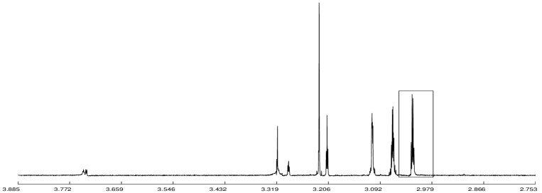
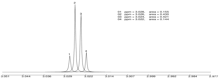
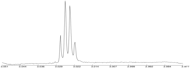
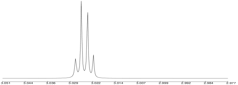
Figure 1: Quantification of NMR spectra. Top: the NMR Fourier spectrum and the ROI. Middle-top: the estimated Lorentian lines in the ROI and their areas. Middle-bottom: the Fourier spectrum in the ROI. Bottom: the sum of the estimated Lorentian lines.

In the top part of fig.1 a ${}^{1}H$ Magnetic Resonance absorption spectrum from a diluted aqueous solution of the tripeptide Glutathione in its reduced form (GSH) is shown. It is computed by taking the discrete Fourier transform (DFT) of a Free Induction Decay (FID) signal of $4096$ data points. In ideal conditions the physical model for the FID is a linear combination with positive weights of complex exponentials. The absorption spectrum is the real part of the Fourier transform of the FID. It turns out that it is given by a linear combination of Lorentian functions. The spectroscopist is interested in estimating the parameters characterizing these Lorentian lines, namely their modes, widths and relative areas which are simply related respectively to the argument of the complex exponentials modeling the FID, to their absolute value and to weights associated to them. In a real experimental setup the ideal conditions are no longer true. Standard methods, implemented on most spectrometers, fit each peak of the absorption spectrum with a Lorentian function. If the peaks are close, a very ill conditioned non linear problem has to be solved which can heavily depend on the interactive choices of the spectroscopist to initialize the procedure. A better alternative is provided by time-domain methods (see e.g.[28, 29]) which exploit the fact that the FID can be modeled by complex exponentials. The problem can still be very ill conditioned. However, if the SNR is large enough, reasonable estimates of the quantities of interest can be obtained by solving the CEAP problem for the FID by the proposed method, which provides a global stable solution and no longer requires critic interaction with the spectroscopist.

The analysis is performed in the interval of the spectrum marked by the rectangle in the top part of fig.1. A quadruplet whose areas are in the ratios $1:3:3:1$ is the theoretical reference. The frequencies are measured in parts per million (ppm). The standard interactive procedure provides an estimate of the areas of the four peaks such that their ratios are $1.02:3.21:3.15:1$. In order to apply the proposed method the FID is first filtered by a pass-band Fourier filter [4, 3]. In the middle-bottom part of the same figure, the absorption spectrum of the filtered FID is shown. When the main peaks of the spectrum are clustered and the clusters are well separated, it is in fact possible to split the analysis by filtering out from the FID all the frequencies but those belonging to a given interval [18]. The filtered FID is given by only $300$ data points and the proposed method was applied to solve the CEAP for it. The results are shown on the middle-top part of fig.1. Four estimated Lorentian lines marked $1-4$ are plotted and their areas are reported in the legend as well their modes in ppm. The ratios of the areas are $1.07:2.98:2.92:1$ which compare favorably with those estimated interactively. On the bottom part of the figure the weighted sum of the four Lorentian lines is plotted. The agreement with the zoomed absorption spectrum on the middle-bottom part is quite good.

3.2 Time series interpolation and extrapolation

In order to apply the proposed method to solve extrapolation problems it is enough to solve a CEAP for the measured data and then evaluate the model on the extrapolation abscissas. To solve an interpolation problem we notice that, in the noiseless case, we can consider the segments of data before and after the missed segment as produced by the same model (1) for a set of indices $k$ displaced by a fixed quantity $q$. It is easy to show that the generalized eigenvalues and eigenvectors are invariant for such a displacement. Therefore we can solve two separate CEAPs for the observed segments, and apply the proposed method to the pooled generalized eigenvalues and eigenvectors. We need only to modify the Vandermonde matrix for computing $c_{j}^{(r)}$ in the last step to take into account the gap in the observations. Assuming that each segment has $n$ observations we have ${\underline{c}}^{(r)}=V^{\dagger}{\underline{a}},$ where

$$V=\left[\begin{array}[]{llll}1&1&\dots&1\\ \xi_{1}^{(r)}&\xi_{2}^{(r)}&\dots&\xi_{\tilde{p}}^{(r)}\\ .&.&\dots&.\\ .&.&\dots&.\\ (\xi_{1}^{(r)})^{n-1}&(\xi_{2}^{(r)})^{n-1}&\dots&(\xi_{\tilde{p}}^{(r)})^{n-1}\\ (\xi_{1}^{(r)})^{n+q-1}&(\xi_{2}^{(r)})^{n+q-1}&\dots&(\xi_{\tilde{p}}^{(r)})^{n+q-1}\\ .&.&\dots&.\\ .&.&\dots&.\\ (\xi_{1}^{(r)})^{2n+q-1}&(\xi_{2}^{(r)})^{2n+q-1}&\dots&(\xi_{\tilde{p}}^{(r)})^{2n+q-1}\end{array}\right]$$

The interpolated values are then obtained by

$${\underline{a}}_{int}=V\hat{{\underline{c}}},\;\;\;V=\left[\begin{array}[]{llll}\hat{\xi}_{1}^{n}&\hat{\xi}_{2}^{n}&\dots&\hat{\xi}_{\hat{p}}^{n}\\ .&.&\dots&.\\ .&.&\dots&.\\ \hat{\xi}_{1}^{n+q-1}&\hat{\xi}_{2}^{n+q-1}&\dots&\hat{\xi}_{\hat{p}}^{n+q-1}\end{array}\right].$$

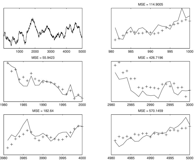
Figure 2: Top left: time series with five missing intervals. True values on each interval (-); interpolated values (+). Total MSE on the first four intervals = 195. Total MSE on the five intervals = 270.

The first example in this class of problems copes with a time series of $5000$ samples with $100$ missing values at times $981-1000,1981-2000,2981-3000,3981-4000,4981-5000$. Therefore we want to solve four interpolation and one extrapolation problems. As the data are synthetic the truth is known and the results obtained by $17$ methods are reported in [8] where the mean squared error (MSE) for the interpolation problems and the interpolation + extrapolation problems are reported. It can be argued that the MSE is not the best discrepancy measure for this data set because a fit with a smoothing cubic spline gives results better than all of the $17$ quoted methods for the interpolation + extrapolation problems and better than $15$ of them for the extrapolation problem. Therefore we want to see how much the proposed method is able to improve on the solution provided by the cubic spline. We then apply the method to the residual obtained by subtracting the smoothing spline from the data. In fig.2 top left the full time series with missing data is plotted. The other plots show the true values and the reconstructed ones on each missed data interval. The $MSE_{100}=270$ and $MSE_{80}=195$ have to be compared with $MSE_{100}=408$ and $MSE_{80}=222$ which are the best results obtained in [8] by two different methods among the $17$ considered.

The second example is illustrated in fig. 3. An audio signal, corresponding to a ringing bell, made up of $50000$ samples at $11025$ Hz is considered. The first $10000$ samples are plotted in the top left part of the figure. A fragment of $1000$ samples are put to zero as shown in the top right part of the figure. The method is applied to interpolate the missing fragment. Two data sets made up of $300$ samples each before and after the missing data are considered as shown in the middle left part of the figure. The results are shown in the middle right part of the figure where $50$ missed data are plotted superimposed to the interpolated values. Even if the fit is not impressive most of the main spectral characteristics of the signal are well reproduced as shown in the bottom part of the figure where the Fourier spectrum of the original complete signal is plotted on the left, and the Fourier spectrum of the complete signal with the missing fragment replaced by the interpolated values is shown on the right. The sound produced by the reconstructed signal is almost undistinguishable from the original one.

	$\sigma$	$RMSE\cite[cite]{[\@@bibref{}{elad}{}{}]}$	$RMSE$
Star shape	1e-3	5.74e-2	3.68e-2
	1e-4	1.74e-2	1.02e-2
	1e-5	1.71e-3	1.05e-3
C shape	1e-3	4.46e-3	4.30e-3
	1e-4	4.51e-4	4.27e-4
	1e-5	4.59e-5	4.28e-5

Table 1: For the star shaped polygon and the C shaped polygon, the RMSE averaged over all the vertices obtained in [12] when $p$ is known and equal to the true value for $\sigma=1e^{-3},1e^{-4},1e^{-5}$ is reported in the third column. In the fourth column the corresponding RMSE obtained by the proposed procedure is reported.

3.3 Shape from moments problems

In [9, 14] it was shown that the $p$ vertices $\xi_{1},\dots,\xi_{p}$ of a non degenerate polygon $\mathcal{P}$ and its complex moments $\mu_{k},k=0,1,\dots,2p-1$ are related by

$$k(k-1)\mu_{k}=k(k-1)\int_{\mathcal{P}}z^{k}dx\;dy=\sum_{j=1}^{p}c_{j}\xi^{j},\;\;\mu_{0}=\mu_{1}=0$$

where

$$c_{j}=\frac{i}{2}\left(\frac{\overline{\xi}_{j-1}-\overline{\xi}_{j}}{\xi_{j-1}-\xi_{j}}-\frac{\overline{\xi}_{j}-\overline{\xi}_{j+1}}{\xi_{j}-\xi_{j+1}}\right)$$

assuming that the vertices are arranged in counterclockwise direction in the order of increasing index and extending the indexing of the $\xi_{j}$ cyclically so that $\xi_{0}=\xi_{p}$, $\xi_{1}=\xi_{p+1}$. Therefore to identify the polygon (i.e. its vertices) from its complex moments is equivalent to solve a CEIP for the data $s_{k}=k(k-1)\mu_{k}$. In [12] several methods for solving this specific problem were compared on two different polygons for $\sigma=10^{-3},10^{-4},10^{-5}$ by a simulation experiment involving $N=100$ independent replications and $n=101$ noisy moments. For comparison, in Table 1 the results obtained by the proposed method and the best among those reported in [12, Tables IV, VIII, bold figures] are reported. The root mean squared error (RMSE) averaged over all parameters $\xi_{j}$ is computed by

$$RMSE=\frac{1}{p}\sum_{k=1}^{p}\sqrt{\frac{1}{N}\sum_{j=1}^{N}|\xi^{(j)}_{k}-\hat{\xi}^{(j)}_{k}|^{2}}.$$

As the best results were obtained in [12] by using GPOF method ([16]) but in one case, also in the proposed procedure the solution of the generalized eigenvalue problem (step 1) was obtained by GPOF with the same setup used in [12]. Therefore $\tilde{p}=p$ is assumed to be known, as in [12], and the $\mathsf{P}$-transform was not computed because all the $p$ estimated clusters were retained. Moreover this was the only example where GPOF was used also for computing $\xi_{j}^{(r)},\;j=1,\dots\tilde{p},r=1,\dots,R$ (slow method). An improvement can be noticed in all cases. In the first column of fig. 4 the estimated $\xi_{j}$ for $\sigma=10^{-4}$ and for the considered polygons are plotted. We notice that in some vertices, the $\xi_{j}$ are so concentrated that they coincide with one point at the used resolution. Next we use the full fast proposed procedure assuming not to know $p$ and putting $\tilde{p}=n/2$. The RMSE averaged over all parameters $\xi_{j}$ and the mean and standard deviation of $\hat{p}$ are reported in Table 2. In the second column of fig. 4 the estimated $\xi_{j}$ for $\sigma=10^{-4}$ and for the considered polygons are plotted.

	$\sigma$	$RMSE$	$p$ mean	$p$ s.d.
Star shape	1e-3	1.07e-1	8	3
	1e-4	7.62e-2	10	3
	1e-5	2.98e-2	11	4
C shape	1e-3	4.13e-2	9	1
	1e-4	2.94e-2	9	2
	1e-5	2.72e-2	9	2

Table 2: For the star shaped polygon and the C shaped polygon, the RMSE averaged over all the vertices obtained in the case of $p$ unknown for $\sigma=1e^{-3},1e^{-4},1e^{-5}$ is reported in the third column. In the fourth and fifth columns the estimated mean and s.d. of $p$ are reported.

4 Conclusion

A new approach for solving a classic inverse ill-posed problem is discussed from the computational point of view. The approach is a perturbative one, therefore it exploits the information generated by solving several closed problems by any standard method which best suits the user’s needs such e.g. numerical quality and/or computational speed. The final results are obtained by an ”averaging” step, hence they are quite stable with respect to noise and, provided that some hyperparameters are properly selected, sensitivity is also preserved, allowing to retrieve features of the signal which are masked by the noise. Several numerical examples are presented which confirm these practical abilities often improving on the results given by known methods.

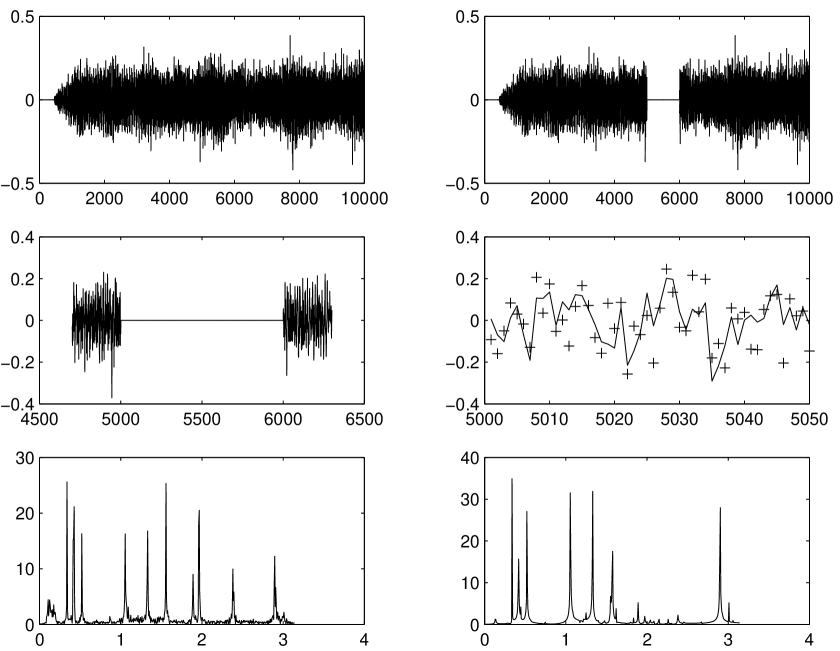
Figure 3: Top left: a segment of an audio signal; top right: the part missed is shown; middle left: the data used to interpolate; middle right: a fraction of the interpolated data (+) are superimposed to the unknown ones (-); bottom left: Fourier spectrum of the missed part; bottom right: Fourier spectrum of the reconstructed data.

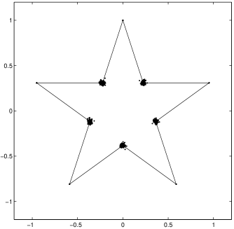
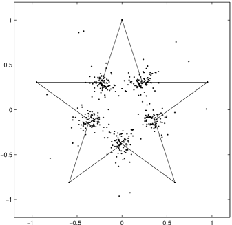
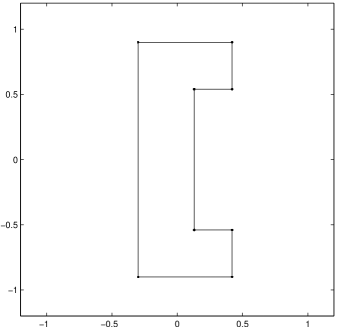
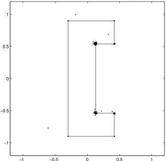
Figure 4: Estimates of the vertices of the star shaped and C shaped polygons obtained by the proposed method on $N=100$ replications with $\sigma=1.e^{-4}$. Left: the true number of vertices is known. Right: the true number of vertices is unknown.

References

- [1] Barone, P. (2008). A new transform for solving the noisy complex exponentials approximation problem, arXiv:0801.1758.
- [2] Barone, P. (2005). On the distribution of poles of Pade’ approximants to the Z-transform of complex Gaussian white noise, J. Approx. Theory 132 224-240.
- [3] Barone, P., March, R. (2001). A novel class of Padé based method in spectral analysis. J. Comput. Methods Sci. Eng. 1 185-211.
- [4] Belkic Dz., Dando P.A., Main J., Taylor H.S. (2000). Three novel high-resolution nonlinear methods for fast signal processing, J.Chem. Phys. 113 (16) 6542–6556
- [5] Bharucha-Reid A.T., Sambandham M. (1986). Random Polynomials. Academic Press, New York.
- [6] Brezinski C., Redivo-Zaglia M. (1991). Extrapolation methods: theory and practice. North Holland, Amsterdam.
- [7] Boutry, G., Elad, M. Golub, G., Milanfar, P. (2005). The generalized eigenvalue problem for nonsquare pencils using a minimal perturbation approach. SIAM J. Sci. Comp.,27,2 582-601.
- [8] Lendasse, A., Oja, E., Simula, O., Verleysen, M. (2004). Time Series Prediction Competition: The CATS Benchmark IJCNN’2004 proceedings International Joint Conference on Neural Networks Budapest (Hungary), 25-29 July 2004, IEEE, 1615-1620.
- [9] Davis, P.J. (1964). Triangle formulas in the complex plane. Math. Comput., 18 569-577.
- [10] Donoho, D.L. (1992). Superresolution via sparsity constraints. SIAM J. Math. Anal., 23,5 1309-1331.
- [11] Hammersley, J.M. (1956). The zeros of a random polynomial. Proc. Berkely Symp. Math. Stat. Probability, 3rd, 2 89-111.
- [12] Elad, M., Milanfar, P., Golub, G. (2004). Shape from Moments - An Estimation Theory Perspective, IEEE Trans. on Signal Processing, 52 1814-1829.
- [13] Golub G.H., Van Loan C.F. (1996). Matrix computations, The Johns Hopkins University Press, Baltimore.
- [14] Golub, G.H., Milanfar, P., Varah, J. (2004). A stable numerical method for inverting shapes from moments. SIAM J. Sci. Comp.,21,4 1222–1243.
- [15] Henrici, P.(1977). Applied and computational complex analysis, vol.I, John Wiley, New York.
- [16] Hua, Y., Sarkar, T.K. (1991). Matrix pencil method for estimating parameters of damped/undamped sinusoids in noise, IEEE TASSP,39 892-900.
- [17] Lemmerling, P., Van Huffel, S. (2002). Structured total least squares: analysis, algorithms and applications. In Van Huffel, S., Lemmerling, P.(Eds.) Total least squares and errors-in-variables modelling. Kluver, Dordrecht, 79–91.
- [18] Neuhauser, D. (1990). Bound state eigenfunctions from wave packets: time-energy resolution, J.Chem. Phys.,93 2611–2616.
- [19] Osborne M.R., Smyth G.K. (1995). A Modified Prony Algorithm for Exponential Function Fitting, SIAM J. Sci. Comput. 16 119-138.
- [20] Prony, R. (1795). Essai expérimental et analytique sur les lois de la dilatabilité de fluides élastiques et sur celles de la force expansive de la vapeur de l’eau et de la vapeur de l’alkool, à différentes températures, Journal de l’École Polytechnique Floréal et Plairial, III, vol.1, n.22, 24-76.
- [21] Paige, C.C. and Saunders, M.A. (1982). LSQR: An Algorithm for Sparse Linear Equations And Sparse Least Squares. ACM Trans. Math. Soft. 8 43-71.
- [22] Saff, E.B., Totik, V. (1997). Logarithmic potentials with external fields, Springer, Berlin
- [23] Scharf, L.L. (1991). Statistical signal processing, Addison-Wesley, Reading.
- [24] Schuermans M., Lemmerling P., De Lathauwer L., Van Huffel S. (2006). The use of total least squares data fitting in the shape-from-moments problem. Signal Processing 86 1109-1115.
- [25] Sitton, G.A.; Burrus, C.S.; Fox, J.W.; Treitel, S. (2003). Factoring very-high-degree polynomials,Signal Processing Magazine IEEE 20 27- 42.
- [26] Stewart, G.W. (2001). Matrix algorithms, vol.2, SIAM, Philadelphia.
- [27] Van Huffel S., Vanderwalle J. (1991). The total least squares problem: computational aspects and analysis, SIAM, Philadelphia.
- [28] Viti, V., Petrucci, C. and Barone, P. (1997). Prony methods in NMR spectroscopy, International Journal of Imaging Systems and Technology 8 565–571.
- [29] Viti, V., Ragona, R., Guidoni, G., Barone, P., Furman, E., Degani, H. (1997). Hormonal -induced modulation in the phosphate metabolites of breast cancer: analysis of in vivo 31P MRS signals with a modified Prony method, Magnetic Resonance in Medicine 38 285–295.
- [30] Wilkinson J.H. (1965). The Algebraic Eigenvalue Problem, Clarendon Press, Oxford.