The lengths distribution of laminar phases
for type-I intermittency in the presence of noise

Abstract

We consider a type of intermittent behavior that occurs as the result of the interplay between dynamical mechanisms giving rise to type-I intermittency and random dynamics. We analytically deduce the laws for the distribution of the laminar phases, with the law for the mean length of the laminar phases versus the critical parameter deduced earlier [PRE 62 (2000) 6304] being the corollary fact of the developed theory. We find a very good agreement between the theoretical predictions and the data obtained by means of both the experimental study and numerical calculations. We discuss also how this mechanism is expected to take place in other relevant physical circumstances.

Introduction

Intermittency is known to be an ubiquitous phenomenon in nonlinear science. Its arousal and main statistical properties have been studied and characterized already since long time ago, and different types of intermittency have been classified as types I–III Bergé et al. (1988); Dubois et al. (1983), on–off intermittency Platt et al. (1993); Heagy et al. (1994); Boccaletti and Valladares (2000); Hramov and Koronovskii (2005), eyelet intermittency Pikovsky et al. (1997); Lee et al. (1998); Boccaletti et al. (2002) and ring intermittency Hramov et al. (2006a).

From the other side, increasing interest has been put recently in the study of the constructive role of noise and fluctuations in nonlinear dynamical systems. In particular, it was discovered that random fluctuations can actually induce some degree of order in a large variety of nonlinear systems Pikovsky and Kurths (1997); Mangioni et al. (1997); Zaikin et al. (2000), and such phenomena were widely observed in relevant physical, chemical and biological circumstances  Neiman and Russell (2002); Zhou et al. (2002, 2003); Boccaletti et al. (2002).

There are no doubts that different types of intermittent behavior may take place in the presence of noise and fluctuations in a wide spectrum of systems, including cases of practical interest for applications in radio engineering, medical, physiological and other applied sciences. It is plausible that such an interaction would originate new types of dynamics. Therefore, the intermittent behavior in the presence of noise has been studied by means of Fokker-Plank equation Hirsch et al. (1982a) and adopting renormalization group analysis Hirsch et al. (1982b), but the characteristic relations were obtained only in the subcritical region, where the intermittent behavior is observed both in the presence of noise and without noise. Recently Kye and Kim (2000), the theoretical consideration of the intermittent behavior in the presence of noise has been considered in the supercritical region (where intermittency is absent in the absence of noise), with the analytical form of the dependence of the mean length of the laminar phases versus the critical parameter being deduced under the assumption of the fixed reinjection probability taken in the form of a $\delta$-function. Moreover, the found analytical law has been verified by means of the experimental observation of the characteristic relations of intermittency in the presence of noise Cho et al. (2002); Kye et al. (2003). At the same time, the other important statistical characteristic of the intermittent behavior, namely, the distribution of the laminar phase lengths, has not been obtained hitherto for the supercritical parameter region.

In this paper we report for the first time the form of the distribution of the lengths of the laminar phases deduced analytically for the type-I intermittency in the presence of noise for the region of the supercritical parameter values. The already known dependence of the mean length of the laminar phases on the criticality parameter Kye and Kim (2000); Cho et al. (2002) follows as a corollary of the carried out research. Moreover, we prove that this dependence obtained in Kye and Kim (2000) under the assumption of the fixed reinjection probability taken in the form of delta-function does not depend practically on the relaminarization properties, and, correspondingly, the obtained expression of the mean length of the laminar phases on the criticality parameter remains correct for different forms of the reinjection probability. The obtained analytical distribution of the laminar phase length is verified by means of both numerical calculations of the model system dynamics and experimental observations.

The structure of the paper is the following. In Sec. I we describe the theory of the type-I intermittency with noise and give the theoretical predictions for the distributions of the laminar phase length. In Sec. II we describe the dynamical systems used to illustrate our conclusions. We show numerically that our theoretical predictions are observed in the different nonlinear systems, including coupled chaotic oscillators near the boundary of the phase synchronization in the case of small detuning of the natural frequencies. Finally, in Sec. III we give the description of the experimental setup for the measurement of the characteristics of the type-I intermittency in the presence of noise. The final conclusions are given in Sec. IV.

I The theory of the type-I intermittency in the presence of noise

The standard model that is used to study the type-I intermittency Bergé et al. (1988) is the one-parameter quadratic map

$$x_{n+1}=f(x_{n})=x_{n}+x_{n}^{2}+\epsilon$$ (1)

where $\epsilon$ is a control parameter. The value of $\epsilon_{c}=0$ corresponds to the saddle-node (tangential) bifurcation when the stable and unstable points touch each other in $x=0$ and disappear.

Below the critical parameter value (i.e., for $\epsilon<\epsilon_{c}$), the stable fixed point is observed, while above $\epsilon_{c}$ a narrow corridor between the function $f(x)$ and the bisector $x_{n+1}=x_{n}$ exists, such that the point representing the state of the map (1) moves along it (Fig. 1). This movement corresponds to the laminar phase, its mean length $T$ being inversely proportional to the square root of $(\epsilon-\epsilon_{c})$, i.e.

$$T\sim(\epsilon-\epsilon_{c})^{-1/2}.$$ (2)

To develop the theory of type-I intermittency in the presence of noise, we consider the same quadratic map (1) with the addition of a stochastic term $\xi_{n}$

$$x_{n+1}=x_{n}+x_{n}^{2}+\epsilon+\xi_{n},$$ (3)

where $\xi_{n}$ is supposed to be a delta-correlated white noise [${\langle\xi_{n}\rangle=0}$, ${\langle\xi_{n}\xi_{m}\rangle=D\delta(n-m)}$].

The influence of the stochastic term $\xi_{n}$ on the behavior of the system is governed by the value of parameter $D$. For positive values of the control parameter $\epsilon$ ($\epsilon>0$), the point corresponding to the behavior of system (3) moves in the iteration diagram along the narrow corridor, its motion being perturbed by the stochastic force. As far as the intensity of the noise is not large, the characteristics of classical type-I intermittency are observed.

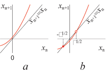
Figure 1: (Color online) The iteration diagram for map (1) (a) $\epsilon>0$ and (b) $\epsilon<0$. The stable and unstable fixed points of (1) are shown by $\bullet$ and $\circ$, respectively

A different scenario occurs for control parameters $\epsilon$ assuming negative values ($\epsilon=-\varepsilon$, where $\varepsilon=|\epsilon|>0$). In this case, the point corresponding to the behavior of system (3) is localized for a long time in the region ${x<x_{c}=\varepsilon^{1/2}}$ and its dynamics is also perturbed by the stochastic force. As soon as the system state point arrives at the boundary $x_{c}=\varepsilon^{1/2}$ due to the influence of noise, a turbulent phase arises, though such kind of events is very rare.

In this case, the behavior of the map (3) differs radically from the dynamics of the system (1), since the turbulent phases are not observed for $\epsilon<0$ if there is no noise. Therefore, such a region of negative values of the $\epsilon$-parameter is the main subject of interest for the type-I intermittency in the presence of noise.

Having supposed that: (i) the value of $\epsilon$ is negative and rather small and (ii) the value of $x$ changes per one iteration insufficiently, we can consider ${(x_{n+1}-x_{n})}$ as the time derivative $\dot{x}$ and undergo from the system with discrete time (3) to the flow system, in the same way as in the case of the classical theory of the type-I intermittency.

Since the stochastic term is present in (3) we have to examine the stochastic differential equation

$$dX=(X^{2}-\varepsilon)\,dt+dW$$ (4)

(where $X(t)$ is a stochastic process, $W(t)$ a one-dimensional Winner process, $\varepsilon=|\epsilon|$) instead of the ordinary differential equation ${dx/dt=x^{2}+\epsilon}$ considered in the classical theory of type I intermittency.

The stochastic differential equation (4) is equivalent to the Fokker-Plank equation

$$\frac{\partial\rho_{X}(x,t)}{\partial t}=-\frac{\partial}{\partial x}((x^{2}-\varepsilon)\rho_{X}(x,t))+\frac{D}{2}\frac{\partial^{2}\rho_{X}(x,t)}{\partial x^{2}}$$ (5)

for the probability density $\rho_{X}(x,t)$ of the stochastic process $X(t)$. Contrarily to what done in Ref.  Kye and Kim (2000) (where the backward Fokker-Plank equation was used), we here consider the forward one that allows us to obtain the explicit form of the distribution of the laminar phase lengths. The chosen initial condition is ${\rho_{X}(x,0)=\delta(x)}$, where $\delta(\cdot)$ is a delta-function. Such choice of the initial form of the probability density $\rho_{X}(x,0)$ corresponds to the beginning of the laminar phase, when the point representing the state of the system (3) is in the place with coordinate $x=0$ at time $t=0$. In other words, we suppose that the reinjection probability is a $\delta$-function

$$P_{in}(x)=\delta(x)$$ (6)

and after the relaminarization process the system is always returned to the state $x=0$. Although the reinjection probability $P_{in}(x)$ is well-known to be important factor and should be taken into account when the statistical properties of the intermittent behavior are studied Kim et al. (1994, 1998), in the considered problem the form of the reinjection probability practically does not influence on the distribution of the laminar phase lengths (and the dependence of the mean laminar phase length on the criticality parameter, respectively), as it will be shown below.

To reduce the number of the control parameters the normalization $z=x/\sqrt{\varepsilon}$, $\tau=t{\sqrt{\varepsilon}}$ may be used, after which Eq. (5) may be rewritten in the form

$$\frac{\partial\rho_{Z}(z,\tau)}{\partial\tau}=-\frac{\partial}{\partial z}((z^{2}-1)\rho_{Z}(z,\tau))+\frac{D^{*}}{2}\frac{\partial^{2}\rho_{Z}(z,\tau)}{\partial z^{2}},$$ (7)

where $D^{*}=D\varepsilon^{-3/2}$, $\rho_{Z}(z,\tau)=\rho_{X}(z{\varepsilon}^{1/2},\tau{\varepsilon}^{-1/2})$.

Since the coordinate of the system state is localized for a long time in the region $z<z_{c}=1$, we suppose that the probability density may be written in the form ${\rho_{Z}(z,\tau)=A(\tau)g(z)}$, ${\forall z\leq 1}$, where $A(\tau)>0$ decreases very slowly as time increases, i.e. $dA/d\tau\approx 0$. The function $g(z)$ should also satisfy the conditions

$$g(z)>0~{}~{}\forall z<1\quad\mathrm{and}\quad\displaystyle\int\limits_{-\infty}^{1}g(z)\,dz<\infty.$$ (8)

Under the mentioned assumption, we consider the ordinary differential equation

$$D^{*}g^{\prime\prime}(z)-2((z^{2}-1)g(z))^{\prime}=0$$ (9)

instead of (7) for the region $z<1$.

This equation is equivalent to

$$D^{*}g^{\prime}(z)-2(z^{2}-1)g(z)+C_{1}=0,$$ (10)

where $C_{1}$ is constant. To solve this equation we use the integrating factor

$$M(z)=\exp\left(-\frac{2}{D^{*}}\left(\frac{z^{3}}{3}-z\right)\right).$$ (11)

The solution of (10) may be found in the form

$$g(z)=\frac{\displaystyle C_{1}\int_{0}^{z}\exp\left(\frac{2}{D^{*}}\left(s-\frac{s^{3}}{3}\right)\right)\,ds+C_{2}}{\displaystyle D^{*}\exp\left(\frac{2}{D^{*}}\left(z-\frac{z^{3}}{3}\right)\right)}.$$ (12)

Since the obtained $g(z)$ satisfies the conditions (8) only if $C_{1}\equiv 0$, the probability density $\rho_{Z}(z,\tau)$ in the region $z<1$ is

$$\rho_{Z}(z,\tau)\simeq A(\tau)\exp\left(-\frac{2}{D^{*}}\left(z-\frac{z^{3}}{3}\right)\right).$$ (13)

The decrease of $A(\tau)$ should be determined by the probability distribution taken in the boundary point $z=1$, i.e., $dA(\tau)/d\tau\sim-\rho_{Z}(1,\tau)$. This assumption may be rewritten as

$$\frac{dA(\tau)}{d\tau}=-kA(\tau)\exp\left(-\frac{4}{3D^{*}}\right),$$ (14)

where $k$ is a proportionality coefficient. Evidently, the decrease of $A(\tau)$ is described by the exponential law

$$A(\tau)=A(0)\exp(-k\eta\tau),\quad\eta=\exp{(-4/(3D^{*}))}.$$ (15)

Having returned to the initial variables $x$ and $t$ we obtain the following expression for the probability density $\rho_{X}(x,t)$

$$\rho_{X}(x,t)\simeq A(t)\exp\left(-\frac{2}{D}\left(\varepsilon x-\frac{x^{3}}{3}\right)\right),$$ (16)

where

$$A(t)=A(0)\exp\left(-\frac{t}{T}\right),$$ (17)

and

$$T=\frac{1}{k\sqrt{\varepsilon}}\exp\left(\frac{4\varepsilon^{3/2}}{3D}\right),$$ (18)

with $A(t)$ being considered as a normalizing factor, i.e.,

$$A(0)\int\limits_{-\infty}^{\sqrt{\varepsilon}}\exp\left(-\frac{2}{D}\left(\varepsilon x-\frac{x^{3}}{3}\right)\right)\,dx=1.$$ (19)

To confirm the assumptions made above and the obtained equations, we have compared the evolution of the probability density $\rho_{X}(x,t)$ given by (16) with the result of the direct numerical calculation of the Fokker-Plank equation (5) with the values of control parameters $\varepsilon=10^{-2}$, $D=2.5\times 10^{-4}$.

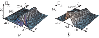
Figure 2: (Color online) The evolution of the probability density $\rho_{X}(x,t)$ obtained by means of the direct numerical integration of Fokker-Plank equation (5), ${\varepsilon=10^{-2}}$, ${D=2.5\times 10^{-4}}$. (a) The initial fragment of the density evolution involving the transient (${0\leq t<t_{tr}}$, $t_{tr}\approx 30$). (b) The long-time evolution of $\rho_{X}(x,t)$, with the transient being omitted, $t\geq 50$

The evolution of the probability density $\rho_{X}(x,t)$ obtined by the numerical calculation of (5) is shown in Fig. 2. One can see that after the very short transient ${0\leq t\leq t_{tr}}$ the probability density $\rho_{X}(x,t)$ arrives the state being close to stationary (Fig. 2 a). After that the value of $\rho_{X}(x,t)$ decreases very slowly (according to the exponential law) with time increasing, with the form of the dependence of the probability density on $x$-coordinate being invariable (Fig. 2 b).

Fig. 3 also shows the profiles of the probability density $\rho_{X}(x,t^{*})$ taken in the different moments of time. It is evident, that after a very short transient (curve 1, $t_{1}^{*}=10$), the density $\rho_{X}(x,t)$ practically does not change when time increases.

Two different profiles $\rho_{X}(x,t^{*})$ corresponding to the time moments $t^{*}_{2}=3\times 10^{1}$ and $t^{*}_{3}=2\times 10^{4}$ (curves 2 and 3, respectively) are very close to each other despite of the very large time interval $\Delta t={t^{*}_{3}-t^{*}_{2}}$ between them. Moreover, they are in very good agreement with the approximated solution $A(0)g(x)$ described by Eq. (16) and shown in Fig. 3 by means of squares. As time goes on, the amplitude of the probability density decreases according to the exponential law, but very slowly (see Fig. 3, curves 4 and 5, $t^{*}_{4}=2.5\times 10^{5}$ and $t^{*}_{5}=10^{6}$, respectively), although the probability density form remains the same for all times.

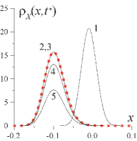
Figure 3: (Color online) The profiles of the probability density $\rho_{X}(x,t^{*})$ taken in the different moments of time $t^{*}$ obtained from the direct numerical calculation of Fokker-Plank equation (5).

Therefore, taking into account the results of the direct numerical calculations of Fokker-Plank equation (5) and the comparison with the obtained approximated solution (16), we come to the conclusion that our assumptions are correct and can be used for the further analysis.

The evolution of the probability density $\rho_{X}(x,t)$ may be considered separately on two time intervals ${0\leq t<t_{tr}}$ and ${t_{tr}\leq t<+\infty}$, respectively. The first time interval corresponds to the transient when the probability density $\rho_{X}(x,t)$ evolves to the form (16) being close to stationary. Only when ${0\leq t<t_{tr}}$ the form of the reinjection probability $P_{in}(x)$ may influence on the evolution of the probability density $\rho_{X}(x,t)$. For $t\geq t_{tr}$ (when the transient is elapsed), the evolution of the probability density is defined completely by Eq. (16) and it does not depend entirely on the reinjection probability $P_{in}(x)$. Since the transient is very short in comparison with the exponential decrease of the probability density $\rho_{X}(x,t)$ we can neglect them and use only the second time interval ${t_{tr}\leq t<+\infty}$ to obtain the statistical characteristics of the type-I intermittent behavior in the presence of noise. It is clear, that in this case the obtained results do not depend on the relaminarization process and the reinjection probability $P_{in}(x)$.

The distribution $p(t)$ of the laminar phase lengths $t$ may be defined from the relationship between $\rho_{X}(x,t)$ and $p(t)$

$$p(t)=-\int\limits_{-\infty}^{\sqrt{\varepsilon}}\frac{\partial\rho_{X}(x,t)}{\partial t}\,dx.$$ (20)

Using relations (16), (17) and (19) one can obtain, that the laminar phase distribution is governed by the exponential law

$$p(t)=T^{-1}\exp\left(-{t/T}\right),$$ (21)

where $T$ defined by Eq. (18) is the mean length of the laminar phases. The obtained expression (18) for the mean length $T$ of the laminar phases is consistent with the formal solution $T\sim\varepsilon^{-1/2}f(\sigma^{2}\varepsilon^{-3/2})$ derived in the previous considerations Hirsch et al. (1982a, b); Crutchfield et al. (1982) and coincides with the formula of $T$ given in Kye and Kim (2000). If the criticality parameter $\varepsilon$ is large enough, the approximate equation ${\ln T\sim D^{-1}\varepsilon^{3/2}}$ may be used (see Kye and Kim (2000) for detail). Based on the consideration carried out above we state that Eqs. (18) and (21) do not depend practically on the relaminarization process properties and may be used for the arbitrary reinjection probability $P_{in}(x)$.

II Sample system dynamics

To verify the obtained theoretical predictions, we consider numerically two different dynamical systems showing type-I intermittency, with a stochastic force being added. As such test systems we have selected (i) the quadratic map and (ii) driven Van der Pol oscillator.

II.1 Quadratic map with stochastic force

We start considering the interplay between type-I intermittency and noise using the quadratic map

$$x_{n+1}=x_{n}^{2}+\lambda+\epsilon+D\xi_{n},\mod 1,$$ (22)

where the “$\mathrm{mod~{}}1$” operation is used to provide the return of the system in the vicinity of the point $x=0$; $\lambda=0.25$, and the probability density of the stochastic variable $\xi$ is distributed uniformly on the interval $\xi\in[-1,1]$. The map (22) may be brought to (3) with the help of a linear variable transformation. If the intensity of noise $D$ is equal to zero the saddle-node bifurcation is observed for $\epsilon=0$. The type-I intermittent behavior is observed for $\epsilon>0$, whereas the stable fixed point takes place for $\epsilon<0$. Having added the stochastic force $D=10^{-7}$ in (22) we can expect that the intermittent behavior may be also observed in the area of the negative values of the criticality parameter $\epsilon$.

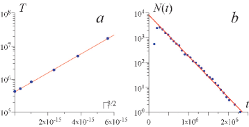
Figure 4: (Color online) (a) The dependence of the mean length $T$ of the laminar phases on the criticality parameter $\varepsilon=|\epsilon|$ ($\epsilon<0$) for (22). The points obtained by the iteration of (22) are shown by symbols ($\bullet$). The theoretical law ${\ln T\sim\varepsilon^{3/2}}$ is shown by the solid line. (b) The distribution of the laminar phase lengths for map (22), the criticality parameter value has been selected as $\varepsilon=10^{-11}$. The theoretical exponential law (21) is shown by the solid line

The dependence of the mean laminar phase length $T$ on the criticality parameter below the point $\epsilon_{c}=0$ is shown in Fig. 4. To compare it with the obtained theoretical prediction ${\ln T\sim D^{-1}\varepsilon^{3/2}}$ the abscissa in Fig. 4, a has been selected in the $\varepsilon^{3/2}$-scale ($\varepsilon=|\epsilon|$, $\epsilon<0$), whereas the ordinate axis is shown in the logarithmic scale. One can see the excellent agreement between theoretical law (18) and data of numerical calculation.

The distribution of the laminar phase lengths is also in very good accordance with the exponential law (21) predicted by the theory of the type-I intermittency with noise (see Fig. 4, b). Note the presence of the small region of the short laminar phase lengths in Fig. 4, b where the deviation from the prescribed exponential law (21) is observed. This region corresponds to the transient ${0\leq t<t_{tr}}$ when the probability density $\rho_{X}(x,t)$ evolves to the form (16) being close to stationary as it was discussed in Sec. I. The existence of this transient time interval does not influence practically on the characteristics (18) and (21) of the intermittent behavior in the presence of noise in the full agreement with the conclusions made above.

So, the intermittent behavior observed in the quadratic map with the stochastic force agrees well with the theoretical predictions obtained in Sec. I. Since the theory of type-I intermittency has been developed on the basis of the model (3) being very close to map (22), it is mandatory to examine another system to ensure that our theoretical conclusions are correct and applicable for a wide spectrum of nonlinear systems.

II.2 Van der Pol oscillator driven by the external harmonic signal in the presence of noise

We consider as a second model the system given by a van der Pol oscillator

$${\ddot{x}-(\lambda-x^{2})\dot{x}+x=A\sin(\omega_{e}t)+D\xi(t)}$$ (23)

driven by an external harmonic signal with the amplitude $A$ and frequency $\omega_{e}$, with an added stochastic term $D\xi(t)$. The values of the control parameters are selected to be $\lambda=0.1$, $\omega_{e}=0.98$. For these control parameters and for $D=0$, the dynamics of the driven van der Pol oscillator becomes synchronized when $A=A_{c}=0.0238$. The probability density of the random variable $\xi(t)$ is

$$p(\xi)=\frac{1}{\sqrt{2\pi}\sigma}\exp\left(-\frac{\xi^{2}}{2\sigma^{2}}\right),$$ (24)

where $\sigma^{2}=1$. To integrate Eq. (23) the one-step Euler method has been used with time step $h=5\times 10^{-4}$, the value of the noise intensity has been fixed as $D=1$.

It is well-known that under certain conditions (i.e., for the periodically forced weakly nonlinear isochronous oscillator), the complex amplitude method may be used to find the solution describing the behavior of oscillator (23) without noise in the form ${x(t)=\mathrm{Re}\,a(t)e^{i\omega t}}$. For the complex amplitude $a(t)$ one obtains the averaged (truncated) equation ${\dot{a}=-i\nu a+a-|a|^{2}a-ik}$, where ${\nu}$ is the frequency mismatch, and $k$ is the (re-normalized) amplitude of the external force. For the small $\nu$ and large $k$, the stable fixed point on the plane of the complex amplitude ${a^{*}=\mathrm{const}}$ corresponds to the synchronous regime, with the synchronization destruction corresponding to the saddle-node bifurcation associated with the global bifurcation of the limit cycle birth Pikovsky et al. (2000); Hramov et al. (2007a). Therefore, below the boundary of the synchronization regime (for small values of the frequency mistuning), the dynamics of the phase difference

$$\Delta\varphi(t)=\varphi(t)-\omega_{e}t$$ (25)

(where $\varphi(t)$ is the phase of the driven oscillator) demonstrates time intervals of phase synchronized motion (laminar phases) persistently and intermittently interrupted by phase slips (turbulent phases) during which the value of $|\Delta\varphi(t)|$ jumps up by $2\pi$. The mean length $T$ of the laminar (synchronous) phases depends on the criticality parameter ${\epsilon=(A_{c}-A)}$ according to the power law (2) corresponding to the type-I intermittency.

If the stochastic term $D\xi(t)$ is added ($D\neq 0$) the manifestation of the regularities of type-I intermittency with noise described above is revealed in the parameter range ${A>A_{c}}$ (see Fig. 5, a). For the negative values of the criticality parameter $\epsilon$ the law ${\ln T\sim D^{-1}\varepsilon^{3/2}}$ is expected to be observed. To make this law evident, the abscissa in Fig. 5, a has been selected in the $\varepsilon^{3/2}$-scale ($\varepsilon=|\epsilon|$) and the ordinate axis $T$ is shown in the logarithmic scale. One can see again the excellent agreement between the numerically calculated data and theoretical prediction (18).

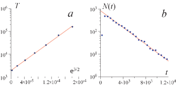
Figure 5: (Color online) (a) The dependencies of the mean length $T$ of the laminar phases on the criticality parameter ${\epsilon=(A_{c}-A)}$ for the driven van der Pol oscillator with the stochastic force (23). The points obtained by the numerical integration of (23) are shown by symbols $\bullet$. The theoretical law ${\ln T\sim\varepsilon^{3/2}}$ is shown by the solid line. (b) The distribution of the laminar phase lengths for the driven van der Pol oscillator, with the amplitude of the external signal $A=0.0245$ being taken above the critical point $A_{c}=0.0238$ ($\epsilon=-7\times 10^{-4}$). The ordinate axis is presented in the logarithmic scale. The theoretical exponential law (21) is shown by the solid line

The distribution of the lengths of the laminar phases $N(t)$ obtained for $A>A_{c}$ also confirms the theoretical results given above. Indeed, the distribution $N(t)$ shown in Fig. 5, b is in the very good accordance with the theoretically predicted exponential law (21), with the small region of the short laminar phase lengths deviating from the exponential law being revealed as well as for the discrete map (22) that corresponds to the short transient taking place after the relaminarization. Again, as for the discrete map considered in Sec. II.1, the existence of this transient time interval does not distort the characteristics of the intermittent behavior observed in the presence of noise.

III Experimental observation of the characteristics of type-I intermittency in the presence of noise

In parallel with the numerical analysis of the type-I intermittent behavior with noise we have also studied experimentally the dynamics of the periodic oscillator driven by the the external harmonic signal in the presence of noise to confirm the theoretical and numerical results given in Sec. I and II. In the experiment we have used the simple electronic oscillator where all parameters (including noise amplitude) may be controlled precisely.

The experimental setup is shown in Fig. 7. The basis element of the scheme we use the generator with the linear feedback and nonlinear converter (NC) Rulkov (1996). The diagram of the nonlinear converter is shown in Fig. 7. The characteristics of nonlinear converter were controlled with resistor $R_{6}$ (see Fig. 7). Since the generator demonstrates both chaotic and periodic oscillations, the control parameters of it have been selected in such a way for the generated signal to be periodic. The frequency of the autonomous periodic oscillations was $8.805$ kHz. As a source of driving harmonic signal the MOTECH-FG503 functional generator (FG) has been used. The behavior of the oscillator driven by the external harmonic signal in the presence of noise was analyzed by means of the Agilent E4402B spectrum analyzer and L-Card L-783 analog–digital converter (ADC) PCI-card with 12-bit resolution.

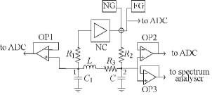
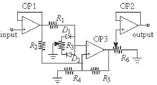
Figure 6: The schematic diagram of the experimental setup. The control parameters have been selected as the following: $R_{1}=10$ Ohm, $R_{2}=630$ Ohm, $R_{3}=56$ Ohm, $L=3.3$ mH, $C=150$ nF, $C_{1}=330$ nF. The operational amplifiers OP1 and OP2 are both of the TL082 type and the operational amplifier OP3 is of the TDA2030 type

Figure 7: The schematic diagram of the nonlinear converter. The control parameters have been selected as the following: $R_{1}=2.7$ kOhm, $R_{2}=7.5$ kOhm, $R_{3}=100$ Ohm, $R_{4}=7.5$ kOhm, $R_{5}=12$ kOhm, $R_{6}=4.7$ kOhm. The diodes $D_{1}$ and $D_{2}$ are of the 1N4148 type. The operational amplifiers OP1 and OP2 are both of the TL082 type and the operational amplifier OP3 is of the LF356N type

The noise generator (NG) shown in Fig. 8, a provides the noise signal being close to Gaussian one Sze (1981). The distribution of noise $p(V)$ is shown in Fig. 8, b. The intensity of noise may be controlled easily by means of the variation of the potentiometer $R_{4}$.

As well as for Van der Pol oscillator driven by the external harmonic signal in the presence of noise (see Sec. II.2) below the boundary of the synchronization regime (for small values of the frequency mistuning) the dynamics of the difference

$$\Delta\varphi(t)=\varphi(t)-\varphi_{e}(t)$$ (26)

between the phase of the driven oscillator $\varphi(t)$ and the phase of the external harmonic signal $\varphi_{e}(t)$ should demonstrate time intervals of phase synchronized motion (laminar phases) persistently and intermittently interrupted by phase slips (turbulent phases) during which the value of $|\Delta\varphi(t)|$ jumps up by $2\pi$. The distribution of the laminar phase length is expected to obey to the exponential law (21) predicted by the theory of the type-I intermittency with noise.

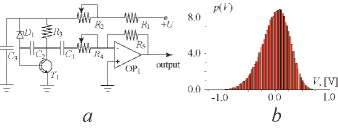
Figure 8: (Color online) (a) The schematic diagram of the noise generator. The control parameters have been selected as the following: $R_{1}=72$ Ohm, $R_{2}=1$ kOhm, $R_{3}=1$ kOhm, $R_{4}=10$ kOhm, $R_{5}=10$ kOhm, $C_{1}=1$ $\mu$F, $C_{2}=0.1$ $\mu$F, $C_{3}=470$ $\mu$F, $U=15$ V. The diode $D_{1}$ is of the BZX79-C11 type. The operational amplifier OP1 is of the TL082 type, the transistor $T_{1}$ is of the BC546B type. (b) The distribution $p(V)$ of noise

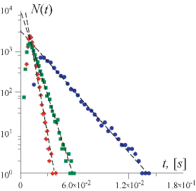
Figure 9: (Color online) The distributions of the laminar phase lengths for the driven periodic oscillator in the presence of noise obtained experimentally. The amplitude $V_{m}$ of the external signal and the noise dispersion $\sigma$ have been selected the following: ($\blacklozenge$) ${V_{m}=170}$ mV, ${\sigma=475.17}$ mV; ($\blacksquare$) ${V_{m}=170}$ mV, ${\sigma=298.11}$ mV; ($\bullet$) ${V_{m}=150}$ mV, ${\sigma=141.72}$ mV. The ordinate axis is presented in the logarithmic scale. The approximations corresponding to the theoretical exponential law (21) are shown by the dashed lines

Since the dependence of the mean laminar phase length on the criticality parameter has already been studied experimentally Cho et al. (2002) in our experiment we focus on the consideration of distribution of the laminar phase lengths. These distributions $N(t)$ obtained experimentally for the different values of the amplitude $V_{m}$ of the external harmonic signal and noise intensity $D$ are shown in Fig. 9. The frequency of the external harmonic signal has been fixed as $f=8.75$ kHz, the values of the amplitude $V$ of the external signal have been selected in such a way for the driven oscillator to be synchronized if the intensity of noise is equal to zero, i.e., $V_{m}>V_{c}$, where $V_{c}=145$ mV is the amplitude of the external signal corresponding to the synchronization threshold. In the presence of noise the phase slips are revealed and the intermittent behavior is observed. One can see that the distributions of the lengths of the laminar phases $N(t)$ are in the very good accordance with the theoretically predicted exponential law (21). The small regions of the short laminar phase lengths where the deviation from the prescribed exponential law (21) is observed also take place as well as in the case of the numerical simulations of the model systems considered in Sec. II. Therefore, we come to conclusion that the experimental observations confirm the obtained theoretical results concerning the type-I intermittent behavior in the presence of noise.

IV Conclusions

In conclusion, we have reported a type of intermittency behavior caused by the cooperation between the deterministic mechanisms and random dynamics. Having examined three sample systems both numerically and experimentally we can conclude that (i) noise induces new features in the intermittent behavior of a system demonstrating type-I intermittency, with new dynamical properties being observed above the former value of the criticality parameter; (ii) the results of numerical simulations and experimental observations are in excellent agreement with the developed theory; (iii) the statistical characteristics of the perturbations of type-I intermittency as well as the relaminarization process properties and the reinjection probability do not seem to play a major role. Though the characterization of the intermittent process has been explicitly derived here for model systems, we expect that the very same mechanism can be observed in many other relevant circumstances where the level of natural noise is sufficient, e.g. in the physiological Hramov et al. (2006b, 2007b) or physical systems Boccaletti et al. (2002).

References

- Bergé et al. (1988) P. Bergé, Y. Pomeau, and C. Vidal, L’Ordre Dans Le Chaos (Hermann, Paris, 1988).
- Dubois et al. (1983) M. Dubois, M.A. Rubio, and P. Bergé, Phys. Rev. Lett. 51, 1446 (1983).
- Platt et al. (1993) N. Platt, E. A. Spiegel, and C. Tresser, Phys. Rev. Lett. 70, 279 (1993).
- Heagy et al. (1994) J. F. Heagy, N. Platt, and S. M. Hammel, Phys. Rev. E 49, 1140 (1994).
- Boccaletti and Valladares (2000) S. Boccaletti and D. L. Valladares, Phys. Rev. E 62, 7497 (2000).
- Hramov and Koronovskii (2005) A. E. Hramov and A. A. Koronovskii, Europhysics Lett. 70, 169 (2005).
- Pikovsky et al. (1997) A. S. Pikovsky, G. V. Osipov, M. G. Rosenblum, M. Zaks, and J. Kurths, Phys. Rev. Lett. 79, 47 (1997).
- Boccaletti et al. (2002) S. Boccaletti, E. Allaria, R. Meucci, and F. T. Arecchi, Phys. Rev. Lett. 89, 194101 (2002).
- Lee et al. (1998) K. J. Lee, Y. Kwak, and T. K. Lim, Phys. Rev. Lett. 81, 321 (1998).
- Hramov et al. (2006a) A. E. Hramov, A. A. Koronovskii, M. K. Kurovskaya, and S. Boccaletti, Phys. Rev. Lett. 97, 114101 (2006a).
- Pikovsky and Kurths (1997) A. S. Pikovsky and J. Kurths, Phys. Rev. Lett. 78, 775 (1997).
- Mangioni et al. (1997) S. Mangioni, R. Deza, H.S. Wio, and R. Toral, Phys. Rev. Lett. 79, 2389 (1997).
- Zaikin et al. (2000) A. A. Zaikin, J. Kurths, and L. Schimansky-Geier, Phys. Rev. Lett. 85, 227 (2000).
- Neiman and Russell (2002) A.B. Neiman and D. F. Russell, Phys. Rev. Lett. 88, 138103 (2002).
- Zhou et al. (2002) C. T. Zhou, J. Kurths, I. Z. Kiss, and J. L. Hudson, Phys. Rev. Lett. 89, 014101 (2002).
- Zhou et al. (2003) C. S. Zhou, J. Kurths, E. Allaria, S. Boccaletti, R. Meucci, and F. T. Arecchi, Phys. Rev. E 67, 015205(R) (2003).
- Hirsch et al. (1982a) J. E. Hirsch, B. A. Huberman, and D. J. Scalapino, Phys. Rev. A 25, 519 (1982a).
- Hirsch et al. (1982b) J. E. Hirsch, M. Nauenberg, and D. J. Scalapino, Phys. Lett. A 87, 391 (1982b).
- Kye and Kim (2000) W.-H. Kye and C.-M. Kim, Phys. Rev. E 62, 6304 (2000).
- Cho et al. (2002) J.-H. Cho, M.-S. Ko, Y.-J. Park, and C.-M. Kim, Phys. Rev. E 65, 036222 (2002).
- Kye et al. (2003) W.-H. Kye, S. Rim, C.-M. Kim, J.-H. Lee, J.-W. Ryu, B.-S. Yeom, and Y.-J. Park, Phys. Rev. E 68, 036203 (2003).
- Kim et al. (1994) C.-M. Kim, O. J. Kwon, E.-K. Lee, and H. Lee, Phys. Rev. Lett. 73, 525 (1994).
- Kim et al. (1998) C.-M. Kim, G.-S. Yim, J.-W. Ryu, and Y.-J. Park, Phys. Rev. Lett. 80, 5317 (1998).
- Crutchfield et al. (1982) J. P. Crutchfield, J. D. Farmer, and B. A. Huberman, Physics Reports 92, 45 (1982).
- Pikovsky et al. (2000) A. S. Pikovsky, M. G. Rosenblum, and J. Kurths, Int. J. Bifurcation and Chaos 10, 2291 (2000).
- Hramov et al. (2007a) A. E. Hramov, A. A. Koronovskii, and M. K. Kurovskaya, Phys. Rev. E 75, 036205 (2007a).
- Rulkov (1996) N. F. Rulkov, Chaos 6, 262 (1996).
- Sze (1981) H. Sze, Physics of Semiconductor Devices (Wiley (New York), 1981).
- Hramov et al. (2006b) A. E. Hramov, A. A. Koronovskii, V. I. Ponomarenko, and M. D. Prokhorov, Phys. Rev. E 73, 026208 (2006b).
- Hramov et al. (2007b) A. E. Hramov, A. A. Koronovskii, V. I. Ponomarenko, and M. D. Prokhorov, Phys. Rev. E 75 (2007b).