Higher-Dimensional Linking Integrals

Abstract.

We derive an integral formula for the linking number of two submanifolds of the n-sphere $S^{n}$, of the product $S^{n}\times\mathbb{R}^{m}$, and of other manifolds which appear as “nice” hypersurfaces in Euclidean space. The formulas are geometrically meaningful in that they are invariant under the action of the special orthogonal group on the ambient space.

1. Introduction

In [G], Carl Friedrich Gauß defined an integral whose purpose was to compute the linking number of two closed curves in Euclidean 3-space. Gauß’s linking integral follows from at least two elementary arguments: one involves thinking of the curves as wires, running a current through one and applying Ampère’s Law, while the other is a straightforward degree-of-map argument (see [E]). The latter extends easily to all Euclidean spaces (as we will see in Section 2), but cannot be directly adapted to spheres. As such, when Dennis DeTurck and Herman Gluck set out to derive integral formulas for the linking number of closed curves in the 3-sphere and in hyperbolic 3-space [DG1], they adapted the first argument, developing steady-state versions of electrodynamics in those spaces.

The integrals defined by Gauß in the case of $\mathbb{R}^{3}$ and by DeTurck and Gluck in the case of $S^{3}$ and $H^{3}$ apply to the simplest of the eight 3-dimensional model geometries and motivate the search for a linking integral in the next simplest geometry, $S^{2}\times\mathbb{R}$. An explicit formula for this case is given in Section 4, but the techniques developed to obtain this formula apply to a much broader class of manifolds, which we call “visible hypersurfaces”.

Call a smooth hypersurface $M^{n}\subset\mathbb{R}^{n+1}$ visible from the point $p$ if each ray from $p$ either misses $M^{n}$ completely, or else meets it just once transversally. We will always arrange things so that $p$ is the origin in $\mathbb{R}^{n+1}$, and simply call our hypersurfaces visible. The principal examples are $S^{n}\subset\mathbb{R}^{n+1}$ and $S^{n}\times\mathbb{R}^{m}\subset\mathbb{R}^{n+m+1}$. Every closed manifold is homotopically equivalent to a visible hypersurface in some Euclidean space. Our main theorem gives explicit linking integrals in all visible hypersurfaces:

Theorem 1.1.

Let $K^{k}$ and $L^{\ell}$ be disjoint, closed, oriented, null-homologous submanifolds of a visible hypersurface $M^{n}\subset\mathbb{R}^{n+1}$ such that $k+\ell=n-1$. Then their linking number is given by

(1) $$Lk(K,L)=\frac{1}{\mathrm{vol}\,S^{n}}\int_{K\times L}\frac{\Omega_{k,\ell}(\alpha)}{|x|^{k+1}|y|^{\ell+1}\sin^{n}\alpha}\,[x,dx,y,dy]$$

where

$$\Omega_{k,\ell}(\alpha)=\int_{\theta=\alpha}^{\pi}\sin^{k}(\theta-\alpha)\sin^{\ell}\theta\,d\theta.$$

Here $\alpha(x,y)$ is the angle between $x\in K$ and $y\in L$, thought of as vectors in $\mathbb{R}^{n+1}$, and the notation $[x,dx,y,dy]$ is as defined in Section 3.

In $\mathbb{R}^{3}$, or equivalently $S^{3}$, the linking number of $K$ with $L$ is defined to be the oriented intersection number of $K$ with a chain $\overline{L}$ bounded by $L$. Extend this definition to higher dimensions by defining the linking number of two submanifolds $K^{k}$ and $L^{\ell}$ to be the oriented intersection number $K\cdot\overline{L}$ of $K$ with a chain $\overline{L}$ bounded by $L$. This intersection number only makes sense when $k$ and $\ell$ are as in Theorem 1.1.

Remark 1.2.

The integrand in (1) is $SO(n+1)$-invariant, meaning that it will be the same for $K$ and $L$ in $M^{n}\subset\mathbb{R}^{n+1}$ as it is for $h(K)$ and $h(L)$ in $h(M)$ for all $h\in SO(n+1)$, whether or not $M^{n}$ is invariant under $h$.

As an immediate corollary to Theorem 1.1, we get an integral formula for the linking number of submanifolds of $S^{n}$ which agrees with the formulas obtained independently and by quite different methods by Kuperberg [K] and DeTurck and Gluck [DG2]:

Theorem 1.3.

Let $K^{k}$ and $L^{\ell}$ be disjoint, closed, oriented submanifolds of the round $n$-sphere $S^{n}$ with $k+\ell=n-1$. Then

$$Lk(K,L)=\frac{1}{\mathrm{vol}\,S^{n}}\int_{K\times L}\frac{\Omega_{k,\ell}(\alpha)}{\sin^{n}\alpha}\,[x,dx,y,dy]$$

where

$$\Omega_{k,\ell}(\alpha)=\int_{\theta=\alpha}^{\pi}\sin^{k}(\theta-\alpha)\sin^{\ell}\theta\,d\theta.$$

Here $\alpha(x,y)$ is the distance in $S^{n}$ from $x\in K$ to $y\in L$.

Remark 1.4.

The integrand in Theorem 1.3 is invariant under orientation-preserving isometries of $S^{n}$.

To prove Theorem 1.1, we first adapt the degree-of-map proof of the Gauß linking integral to get an integral formula for the linking number of closed submanifolds of $\mathbb{R}^{N}$ for all $N$. Then, for submanifolds $K$ and $L$ of the visible hypersurface $M^{n}\subset\mathbb{R}^{n+1}$, we associate to $K$ a family of closed singular submanifolds $CK_{R}\subset\mathbb{R}^{n+1}$ of one higher dimension for $R\in(1,\infty)$. We apply the integral formula in $\mathbb{R}^{n+1}$ to the pair $(CK_{R},L)$ and, after taking an appropriate limit, deduce the integral in Theorem 1.1.

Acknowledgments

We owe a considerable debt of gratitude to Dennis DeTurck and Herman Gluck for introducing us to linking integrals and for many helpful and illuminating conversations.

2. A linking integral for $\mathbb{R}^{N}$

To obtain a linking integral formula for $\mathbb{R}^{N}$, we directly adapt the degree-of-map proof of the Gauß linking integral.

Let $K^{k},L^{\ell}\subset\mathbb{R}^{N}$ be disjoint, closed, oriented submanifolds such that $k+\ell=N-1$. Let $x:\mathbb{R}^{k}\to K\subset\mathbb{R}^{N}$ and $y:\mathbb{R}^{\ell}\to L\subset\mathbb{R}^{N}$ be oriented local coordinates for $K$ and $L$, where ${\bf s}=(s_{1},\ldots,s_{k})$ and ${\bf t}=(t_{1},\ldots,t_{\ell})$ give the coordinates on $\mathbb{R}^{k}$ and $\mathbb{R}^{\ell}$, respectively. Then, up to sign, we can express $Lk(K,L)$ as the degree of a map:

Lemma 2.1.

If $K$ and $L$ are as above and $f:K\times L\to S^{N-1}$ is given by

$$f(x,y)=\frac{x-y}{|x-y|},$$

then the degree of the map $f$ is equal to $(-1)^{N}$ times the linking number of $K$ and $L$. In other words, if $\omega$ is a volume form on $S^{N-1}$, then

$$Lk(K,L)=\frac{(-1)^{N}}{\mathrm{vol}\,S^{N-1}}\int_{K\times L}f^{*}\omega.$$

The idea of the proof of Lemma 2.1 is the following: if we change $K$ by a homology in the complement of $L$ (or vice versa), the degree of $f$ remains unchanged. Hence, we can replace $K$ and $L$ by pairwise meridional round $k$- and $\ell$-spheres (with multiplicity). In this special case, it is a straightforward exercise to check that the degree of $f$ is $(-1)^{N}$ times the linking number.

With Lemma 2.1 in hand, we turn to finding a linking integral for submanifolds of $\mathbb{R}^{N}$. In the following theorem and throughout the rest of this paper we will use the notation $(v_{1},\ldots,v_{N})$ to denote the $N\times N$ matrix with rows given by the vectors $v_{1},\ldots,v_{N}\in\mathbb{R}^{N}$.

Theorem 2.2.

With $K$ and $L$ as above,

(2) $$Lk(K,L)=\frac{(-1)^{k+1}}{\mathrm{vol}\,S^{N-1}}\int_{K\times L}\frac{1}{|x-y|^{N}}\,[x-y,dx,dy],$$

where

$$[x-y,dx,dy]=\det\left(x-y,\frac{\partial x}{\partial s_{1}},\cdots,\frac{\partial x}{\partial s_{k}},\frac{\partial y}{\partial t_{1}},\cdots,\frac{\partial y}{\partial t_{\ell}}\right)d{\bf s}\,d{\bf t}.$$

Remark 2.3.

Theorem 2.2 is a direct generalization of the original Gauß linking integral,

$$Lk(K,L)=\frac{1}{4\pi}\int_{K\times L}\frac{x-y}{|x-y|^{3}}\cdot\left(\frac{dx}{ds}\times\frac{dy}{dt}\right)ds\,dt,$$

since $\frac{1}{|x-y|^{3}}[x-y,dx,dy]$ is equal to the triple product in the above integrand.

Proof.

By Lemma 2.1, it suffices to show that

(3) $$f^{*}\omega=\frac{(-1)^{\ell}}{|x-y|^{N}}\,[x-y,dx,dy]$$

where $\omega$ is the volume form on $S^{N-1}$.

For $S^{N-1}$ embedded in $\mathbb{R}^{N}$ in the usual way, we can give an explicit formula for the volume form $\omega$ on $S^{N-1}$: if $p\in S^{N-1}$ and $V_{1},\ldots,V_{N-1}\in T_{p}S^{N-1}$, then $\omega_{p}(V_{1},\ldots,V_{N-1})$ is equal to the volume of the parallelpiped spanned by the vectors $p,V_{1},\ldots,V_{N-1}$ in $\mathbb{R}^{N}$:

$$\omega_{p}(V_{1},\ldots,V_{N-1})=\det(p,V_{1},\ldots,V_{N-1}).$$

Therefore,

(4) $$f^{*}\omega\left(\frac{\partial}{\partial s_{1}},\ldots,\frac{\partial}{\partial s_{k}},\frac{\partial}{\partial t_{1}},\ldots,\frac{\partial}{\partial t_{\ell}}\right)=\det\left(f(x,y),\frac{\partial f}{\partial s_{1}},\ldots,\frac{\partial f}{\partial s_{k}},\frac{\partial f}{\partial t_{1}},\ldots,\frac{\partial f}{\partial t_{\ell}}\right).$$

Note that, if $f(x,y)=(f_{1}(x,y),\dots,f_{N}(x,y))$, then

(5) $$\frac{\partial f_{i}}{\partial s_{\eta}}=\frac{\partial}{\partial s_{\eta}}\left(\frac{x_{i}-y_{i}}{|x-y|}\right)=\frac{\frac{\partial x_{i}}{\partial s_{\eta}}}{|x-y|}+(x_{i}-y_{i})\frac{\partial}{\partial s_{\eta}}\left(\frac{1}{|x-y|}\right)$$

and

(6) $$\frac{\partial f_{i}}{\partial t_{\nu}}=\frac{\partial}{\partial t_{\nu}}\left(\frac{x_{i}-y_{i}}{|x-y|}\right)=\frac{-\frac{\partial y_{i}}{\partial t_{\nu}}}{|x-y|}+(x_{i}-y_{i})\frac{\partial}{\partial t_{\nu}}\left(\frac{1}{|x-y|}\right).$$

However, since, in (4), $f_{i}(x,y)=\frac{x_{i}-y_{i}}{|x-y|}$ is in the same column as both $\frac{\partial f_{i}}{\partial s_{\eta}}$ and $\frac{\partial f_{i}}{\partial t_{\nu}}$, the second terms in both (5) and (6) contribute nothing to the determinant.

Thus, combining (4), (5) and (6), we see that

$$f^{*}\omega\left(\frac{\partial}{\partial s_{1}},\ldots,\frac{\partial}{\partial s_{k}},\frac{\partial}{\partial t_{1}},\ldots,\frac{\partial}{\partial t_{\ell}}\right)=\frac{(-1)^{\ell}}{|x-y|^{N}}\det\left(x-y,\frac{\partial x}{\partial s_{1}},\ldots,\frac{\partial x}{\partial s_{k}},\frac{\partial y}{\partial t_{1}},\ldots,\frac{\partial y}{\partial t_{\ell}}\right),$$

which is just a restatement of (3). ∎

3. A linking integral for visible hypersurfaces

In this section, we prove Theorem 1.1 by making use of the linking integral in $\mathbb{R}^{n+1}$. We assume $n>1$; in the special case that $n=1$, $K$ and $L$ are both zero-dimensional and Theorem 1.1 can be verified directly. To set notation, let $K^{k}$ and $L^{\ell}$ be disjoint, closed, oriented, null-homologous submanifolds of the visible hypersurface $M^{n}\subset\mathbb{R}^{n+1}$ such that $k+\ell=n-1$. We use $x$, $y$, ${\bf s}$ and ${\bf t}$ as in Section 2 and use $[x,dx,y,dy]$ to denote

$$\det\left(x,\frac{\partial x}{\partial s_{1}},\ldots,\frac{\partial x}{\partial s_{k}},y,\frac{\partial y}{\partial t_{1}},\ldots,\frac{\partial y}{\partial t_{\ell}}\right)d{\bf s}\,d{\bf t}.$$

Since the linking number is symmetric up to sign, we may assume, without loss of generality, that $k\leq\ell$.

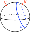
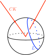
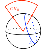
The key idea is to derive an integral formula for linking numbers in $M^{n}$ from the one in $\mathbb{R}^{n+1}$ appearing in Theorem 2.2. This is illustrated in Figure 1 in the case $M^{n}=S^{n}$.

(a)

(b)

(c)

Figure 1.

In Figure 1(a), we see the cycles $K$ and $L$ in $S^{n}$. In Figure 1(b), we see the cycles $CK$ and $L$ in $\mathbb{R}^{n+1}$, where $CK:=\{\tau x:x\in K,0\leq\tau<\infty\}$ is the (half-infinite) cone over $K$.

We intend to take the formula for $Lk(CK,L)$ in $\mathbb{R}^{n+1}$, expressed as an integral over $CK\times L$, and partially integrate it over the rays $0\leq\tau<\infty$ to reduce it to an integral over $K\times L$ for $Lk(K,L)$ in $S^{n}$.

The noncompactness of $CK$ raises questions about the meaning of $Lk(CK,L)$ and the convergence of the linking integral, which we handle by approximation as follows. In Figure 1(c), we see the cycles $CK_{R}$ and $L$ in $\mathbb{R}^{n+1}$, where $CK_{R}$ consists of the truncated cone $\{\tau x:x\in K,0\leq\tau\leq R\}$, capped off by the scaled version $R\overline{K}$ of a chain $\overline{K}$ in $M$ bounded by $K$. We see that $Lk_{\mathbb{R}^{n+1}}(CK_{R},L)=Lk_{S^{n}}(K,L)$ because $CK_{R}$ meets a chain $\overline{L}$ bounded by $L$ exactly as $K$ does. We then show that the integral for $Lk(CK_{R},L)$ converges to the integral for $Lk(CK,L)$ as $R\to\infty$ because the contribution to the linking integral coming from the cap $R\overline{K}$ vanishes as $R\to\infty$.

Lemma 3.1.

With $K$ and $L$ as in Theorem 1.1 and provided $n>1$,

(7) $$Lk(K,L)=\frac{(-1)^{k}}{\mathrm{vol}\,S^{n}}\int_{CK\times L}\frac{1}{|\tau x-y|^{n+1}}\,[\tau x-y,d(\tau x),dy].$$

Proof.

We will interpret (7) as the limit of integrals given by applying Theorem 2.2 to the family of closed, singular manifolds $CK_{R}$, $1<R<\infty$. By construction, $Lk(K,L)=Lk(CK_{R},L)$ for all $R>1$. Since the singularities of $CK_{R}$ have measure zero, we can use Theorem 2.2 to compute $Lk(CK_{R},L)$:

$$Lk(CK_{R},L) =\frac{(-1)^{k+2}}{\mathrm{vol}\,S^{n}}\int_{CK_{R}\times L}\frac{1}{|\xi-y|^{n+1}}\,[\xi-y,d\xi,dy]$$

(8) $$=\frac{(-1)^{k+2}}{\mathrm{vol}\,S^{n}}\int_{\{\tau x:x\in K,\tau\in[0,R]\}\times L}\frac{1}{|\tau x-y|^{n+1}}\,[\tau x-y,d(\tau x),dy]$$

$$\qquad+\frac{(-1)^{k+2}}{\mathrm{vol}\,S^{n}}\int_{\overline{K}\times L}\frac{1}{|Rz-y|^{n+1}}\,[Rz-y,d(Rz),dy].$$

As $R\to\infty$, the first term on the right hand side of (8) approaches the right hand side of (7). Therefore, to complete the proof we need only show that

(9) $$\frac{(-1)^{k+2}}{\mathrm{vol}\,S^{n}}\int_{\overline{K}\times L}\frac{1}{|Rz-y|^{n+1}}\,[Rz-y,d(Rz),dy]\to 0$$

as $R\to\infty$. However, as $R$ gets large the numerator in the integrand grows like $R^{k+2}$, whereas the denominator grows like $R^{n+1}$. The assumptions $k\leq\ell$ and $n>1$ imply that $k+2<n+1$. Therefore, the integrand vanishes in the limit, implying (9) and completing the proof.

∎

Now we are ready to prove the linking integral formula for $M^{n}$.

Proof of Theorem 1.1.

By Lemma 3.1,

(10) $$Lk(K,L)=\frac{(-1)^{k}}{\mathrm{vol}\,S^{n}}\int_{CK\times L}\frac{1}{|\tau x-y|^{n+1}}\,[\tau x-y,d(\tau x),dy].$$

Focusing first on $[\tau x-y,d(\tau x),dy]$, we see that

$$[\tau x-y,d(\tau x),dy] =d\tau\wedge\left[\det\left(\tau x-y,x,\tau\frac{\partial x}{\partial s_{1}},\ldots,\tau\frac{\partial x}{\partial s_{k}},\frac{\partial y}{\partial t_{1}},\ldots,\frac{\partial y}{\partial t_{\ell}}\right)d{\bf s}\,d{\bf t}\right]$$

$$=(-1)^{k}\tau^{k}d\tau\wedge[x,dx,y,dy].$$

Combining this with (10), we see that

$$Lk(K,L)=\frac{1}{\mathrm{vol}\,S^{n}}\int_{K\times L}\int_{\tau=0}^{\infty}\frac{\tau^{k}}{|\tau x-y|^{n+1}}\,d\tau\wedge[x,dx,y,dy].$$

Therefore, it suffices to show that

(11) $$\int_{\tau=0}^{\infty}\frac{\tau^{k}}{|\tau x-y|^{n+1}}\,d\tau=\frac{1}{|x|^{k+1}|y|^{\ell+1}\sin^{n}\alpha}\int_{\theta=\alpha}^{\pi}\sin^{k}(\theta-\alpha)\sin^{\ell}\theta\,d\theta.$$

Figure 2.

As illustrated in Figure 2, we can re-write $|\tau x-y|^{n+1}$ as

$$|\tau x-y|^{n+1}=\left(|y|^{2}+\tau^{2}|x|^{2}-2\tau\langle x,y\rangle\right)^{\frac{n+1}{2}}=\left(|y|^{2}+\tau^{2}|x|^{2}-2\tau|x||y|\cos\alpha\right)^{\frac{n+1}{2}},$$

where we recall that $\alpha(x,y)$ is the angle (in $\mathbb{R}^{n+1}$) formed by $x$ and $y$.

Now make the substitution $u=\tau-\frac{|y|}{|x|}\cos\alpha$ in the left hand side of (11) to get

$$\frac{1}{|x|^{n+1}}\int_{-\frac{|y|}{|x|}\cos\alpha}^{\infty}\frac{\left(u+\frac{|y|}{|x|}\cos\alpha\right)^{k}}{\left(u^{2}+\frac{|y|^{2}}{|x|^{2}}\sin^{2}\alpha\right)^{\frac{n+1}{2}}}\,du.$$

Substituting $-\frac{|y|}{|x|}\sin\alpha\cot\theta$ for $u$ and simplifying yields

$$\frac{1}{|x|^{k+1}|y|^{\ell+1}\sin^{n}\alpha}\int_{\theta=\alpha}^{\pi}(\cos\alpha-\sin\alpha\cot\theta)^{k}\sin^{n-1}\theta\,d\theta\\ =\frac{1}{|x|^{k+1}|y|^{\ell+1}\sin^{n}\alpha}\int_{\theta=\alpha}^{\pi}\sin^{k}(\theta-\alpha)\sin^{\ell}\theta\,d\theta,$$

which is the right hand side of (11), completing the proof of the theorem. ∎

4. A few examples

To see that Theorem 1.1 is useful in practice, we apply it to some prototypical examples. First, we note that Theorem 1.3 can be used to recover the linking integral in $S^{3}$. In this case, $k=\ell=1$, so

$$\Omega_{1,1}(\alpha) =\int_{\alpha}^{\pi}\sin(\theta-\alpha)\sin\theta\,d\theta$$

$$=\frac{(\pi-\alpha)\cos\alpha+\sin\alpha}{2}.$$

Thus, the linking number of disjoint closed curves $K$ and $L$ in $S^{3}$ is given by

$$Lk(K,L)=\frac{1}{4\pi^{2}}\int_{K\times L}\frac{(\pi-\alpha)\cos\alpha+\sin\alpha}{\sin^{3}\alpha}\,[x,dx,y,dy].$$

This is equivalent to the formulas obtained by DeTurck and Gluck in [DG1] and Kuperberg in [K].

This same computation for disjoint, closed curves in $S^{2}\times\mathbb{R}$ yields the linking formula

$$Lk(K,L)=\frac{1}{4\pi^{2}}\int_{K\times L}\frac{(\pi-\alpha)\cos\alpha+\sin\alpha}{|x|^{2}|y|^{2}\sin^{3}\alpha}\,[x,dx,y,dy].$$

As noted in the introduction, the integrand in this linking integral formula is invariant under the action of $SO(4)$ on the ambient Euclidean space, so it is invariant under rotations in the $S^{2}$ factor, though not necessarily under translations in the $\mathbb{R}$ factor. This is in contrast to the formulas of Gauß in $\mathbb{R}^{3}$ and DeTurck and Gluck in $S^{3}$ and $H^{3}$, whose integrands are invariant under the full group of orientation-preserving isometries of their respective manifolds.

Now we turn to more concrete examples. Let $K=S^{k}$ and $L=S^{\ell}$ be two great spheres contained in $S^{k+\ell+1}$ at constant geodesic distance $\pi/2$. Up to ambient isometry, we may as well take $K$ as the unit sphere in the first $k+1$ coordinates in $\mathbb{R}^{k+\ell+2}$ and $L$ as the unit sphere in the last $\ell+1$ coordinates. Then, by construction, $Lk(K,L)=1$; we want to see that Theorem 1.3 gives the same result.

To simplify the computation, we recall the following fact relating integrals of sines and cosines to the volumes of spheres:

Fact 4.1.

$$\mathrm{vol}\,S^{k+\ell+1}=\mathrm{vol}\,S^{k}\ \mathrm{vol}\,S^{\ell}\int_{0}^{\pi/2}\cos^{k}\theta\sin^{\ell}\theta\,d\theta.$$

Fact 4.1 follows from viewing $S^{k+\ell+1}$ as the spherical join of orthogonal great spheres $S^{k}$ and $S^{\ell}$ and computing the volume in the natural coordinates that result from this identification.

In our example, since $K$ and $L$ are at constant geodesic distance $\pi/2$, the above fact implies that $\Omega_{k,\ell}$ has the form

$$\Omega_{k,\ell}(\alpha) =\int_{\pi/2}^{\pi}\sin^{k}(\theta-\pi/2)\sin^{\ell}\theta\,d\theta$$

$$=\int_{0}^{\pi/2}\cos^{k}\theta\sin^{\ell}\theta\,d\theta$$

$$=\frac{\mathrm{vol}\,S^{k+\ell+1}}{\mathrm{vol}\,S^{k}\ \mathrm{vol}\,S^{\ell}}.$$

Therefore,

$$Lk(K,L) =\frac{1}{\mathrm{vol}\,S^{k+\ell+1}}\int_{K\times L}\frac{1}{\sin^{k+\ell+1}(\pi/2)}\frac{\mathrm{vol}\,S^{k+\ell+1}}{\mathrm{vol}\,S^{k}\ \mathrm{vol}\,S^{\ell}}\,[x,dx,y,dy]$$

$$=\frac{1}{\mathrm{vol}\,S^{k}\ \mathrm{vol}\,S^{\ell}}\int_{K\times L}[x,dx,y,dy]$$

$$=\frac{1}{\mathrm{vol}\,S^{k}\ \mathrm{vol}\,S^{\ell}}\mathrm{vol}\,S^{k}\ \mathrm{vol}\,S^{\ell}$$

$$=1.$$

The second-to-last equality follows because, since $K$ is contained in the $\mathbb{R}^{k+1}$ factor and $L$ is contained in the $\mathbb{R}^{\ell+1}$ factor of $\mathbb{R}^{k+\ell+2}=\mathbb{R}^{k+1}\times\mathbb{R}^{\ell+1}$, $[x,dx,y,dy]=[x,dx]\wedge[y,dy]=d\mathrm{Vol}_{S^{k}}\wedge d\mathrm{Vol}_{S^{\ell}}$.

Finally, we use Theorem 1.1 to compute the simplest example in $S^{2}\times\mathbb{R}$. Thinking of the $\mathbb{R}$ factor as time, let $K$ be the instantaneous equator on the $S^{2}$ factor at time 0 and let $L$ be the union of the eternal north pole traversed positively in time with the eternal south pole traversed negatively in time. We can think of $L$ as the limit when $\tau\to\infty$ of the curves $L_{\tau}$ shown in Figure 3.

Figure 3. $K$ and $L_{\tau}$ in $S^{2}\times\mathbb{R}$

With this choice of $K$ and $L$, $\alpha$ is again equal to $\pi/2$ for all $x\in K$ and $y\in L$. Therefore,

$$\Omega_{1,1}(\alpha)=\frac{\mathrm{vol}\,S^{3}}{\mathrm{vol}\,S^{1}\ \mathrm{vol}\,S^{1}}=\frac{\mathrm{vol}\,S^{3}}{4\pi^{2}}.$$

Thus,

$$Lk(K,L) =\frac{1}{\mathrm{vol}\,S^{3}}\int_{K\times L}\frac{\mathrm{vol}\,S^{3}}{|y|^{2}4\pi^{2}}\,[x,dx,y,dy]$$

$$=2\cdot\frac{1}{4\pi^{2}}\int_{-\infty}^{\infty}\int_{0}^{2\pi}\frac{1}{1+t^{2}}\det\left(\begin{array}[]{cccc}\cos s&\sin s&0&0\\ -\sin s&\cos s&0&0\\ 0&0&1&t\\ 0&0&0&1\end{array}\right)ds\,dt$$

$$=\frac{1}{2\pi^{2}}\int_{-\infty}^{\infty}\int_{0}^{2\pi}\frac{1}{1+t^{2}}\,ds\,dt$$

$$=1.$$

In the second equality we use the symmetry of $L$ to eliminate the integral over the south pole component by doubling the contribution of the north pole component.

References

• [DG1] Dennis DeTurck and Herman Gluck: Electrodynamics and the Gauss linking integral on the 3-sphere and in hyperbolic 3-space. To appear, J. Math. Phys. arXiv:math/0510388v1 [math.GT]
• [DG2] Dennis DeTurck and Herman Gluck: Linking integrals in the nn-sphere. Preprint, 2008.
• [E] Moritz Epple: Orbits of asteroids, a braid, and the first link invariant. Math. Intelligencer, 20(1):45-52, 1998.
• [G] Carl Friedrich Gauß: Integral Formula for Linking Number. In Zur mathematischen theorie der electrodynamische wirkungen (Collected Works, Vol. 5), p. 605. Koniglichen Gesellschaft des Wissenschaften, Göttingen, 2nd edition, 1833.
• [K] Greg Kuperberg: From the Mahler conjecture to Gauss linking forms. Preprint, 2006. arXiv:math/0610904v2 [math.MG]