Global dynamics of coupled standard maps

Abstract

Understanding the dynamics of multi–dimensional conservative dynamical systems (Hamiltonian flows or symplectic maps) is a fundamental issue of nonlinear science. The Generalized ALignment Index (GALI), which was recently introduced and applied successfully for the distinction between regular and chaotic motion in Hamiltonian systems sk:6 , is an ideal tool for this purpose. In the present paper we make a first step towards the dynamical study of multi–dimensional maps, by obtaining some interesting results for a 4–dimensional (4D) symplectic map consisting of $N=2$ coupled standard maps Kan:1 . In particular, using the new GALI₃ and GALI₄ indices, we compute the percentages of regular and chaotic motion of the map equally reliably but much faster than previously used indices, like GALI₂ (known in the literature as SALI).

1 Definition and behavior of GALI

Let us first briefly recall the definition of GALI and its behavior for regular and chaotic motion, adjusting the results obtained in sk:6 to symplectic maps. Considering of a $2N$–dimensional map, we follow the evolution of an orbit (using the equations of the map) together with $k$ initially linearly independent deviation vectors of this orbit $\overrightarrow{\nu}_{1},\overrightarrow{\nu}_{2},...,\overrightarrow{\nu}_{k}$ with $2\leq k\leq 2N$ (using the equations of the tangent map). The Generalized Alignment Index of order $k$ is defined as the norm of the wedge or exterior product of the $k$ unit deviation vectors:

$$GALI_{k}(i)=\parallel\hat{\nu}_{1}(i)\wedge\hat{\nu}_{2}(i)\wedge...\wedge\hat{\nu}_{k}(i)\parallel$$ (1)

and corresponds to the volume of the generalized parallelepiped, whose edges are these $k$ vectors. We note that the hat ($\,\hat{}\,$) over a vector denotes that it is of unit magnitude and that $i$ is the discrete time.

In the case of a chaotic orbit all deviation vectors tend to become linearly dependent, aligning in the direction of the eigenvector which corresponds to the maximal Lyapunov exponent and GALI_k tends to zero following an exponential law $\sim e^{-[(\sigma_{1}-\sigma_{2})+(\sigma_{1}-\sigma_{3})+...+(\sigma_{1}-\sigma_{k})]i}$, where $\sigma_{1},\ldots,\sigma_{k}$ are approximations of the first $k$ largest Lyapunov exponents. In the case of regular motion on the other hand, all deviation vectors tend to fall on the $N$–dimensional tangent space of the torus on which the motion lies. Thus, if we start with $k\leq N$ general deviation vectors they will remain linearly independent on the $N$–dimensional tangent space of the torus, since there is no particular reason for them to become aligned. As a consequence GALI_k remains practically constant for $k\leq N$. On the other hand, GALI_k tends to zero for $k>N$, since some deviation vectors will eventually become linearly dependent, following a particular power law, i. e. $GALI_{k}(i)\sim i^{2(N-k)}$.

2 Dynamical study of a 4D standard map

As a model for our study we consider the 4D symplectic map:

$$\begin{array}[]{lll}x_{1}^{\prime}&=&x_{1}+x_{2}^{\prime}\qquad x_{2}^{\prime}=x_{2}+\frac{K}{2\pi}\sin(2\pi x_{1})-\frac{B}{2\pi}\sin[2\pi(x_{3}-x_{1})]\\ x_{3}^{\prime}&=&x_{3}+x_{4}^{\prime}\qquad x_{4}^{\prime}=x_{4}+\frac{K}{2\pi}\sin(2\pi x_{3})-\frac{B}{2\pi}\sin[2\pi(x_{1}-x_{3})]\\ \end{array}\,(mod\,1),$$ (2)

which consists of two coupled standard maps Kan:1 and is a typical nonlinear system, in which regions of chaotic and regular dynamics are found to coexist. In our study we fix the parameters of the map (2) to $K=0.5$ and $B=0.05$.

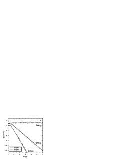
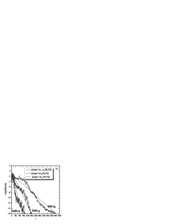
Figure 1: The evolution of GALI_k, $k=2,3,4$, with respect to the number of iterations $i$ for a) the regular orbit R and b) the chaotic orbit C. The plotted lines correspond to functions proportional to $n^{-2}$, $n^{-4}$ in a) and to $e^{-(\sigma_{1}-\sigma_{2})i}$, $e^{-2\sigma_{1}i}$, $e^{-4\sigma_{1}i}$ for $\sigma_{1}=0.070$, $\sigma_{2}=0.008$ in b).

In Fig. 1, we show the behavior of GALIs for two different orbits: a regular orbit R with initial conditions $(x_{1},x_{2},x_{3},x_{4})=(0.55,0.10,0.54,0.01)$ (Fig. 1a), and a chaotic orbit C with initial conditions $(x_{1},x_{2},x_{3},x_{4})=(0.55,0.10,0.005,0.01)$ (Fig. 1b). The positive Lyapunov exponents of orbit C were found to be $\sigma_{1}\approx 0.070$, $\sigma_{2}\approx 0.008$. From the results of Fig. 1 we see that the evolution of GALIs is described very well by the theoretically obtained approximations presented in Sect. 1.

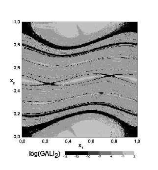
Figure 2: Regions of different values of the GALI₂ (left panel) and GALI₄ (right panel) for a grid of $500\times 500$ initial conditions on the subspace $x_{3}=0.54$, $x_{4}=0.01$ of map (2) for $K=0.5$ and $B=0.05$.

Let us now turn our attention to the study of the global dynamics of map (2). From the results Fig. 1 we conclude that in the case of 4D maps, GALI₂ has different behavior for regular and chaotic orbits. In particular, GALI₂ tends exponentially to zero for chaotic orbits (GALI${}_{2}\sim e^{-(\sigma_{1}-\sigma_{2})i}$) while it fluctuates around non–zero values for regular orbits. This difference in the behavior of the index can be used to obtain a clear distinction between regular and chaotic orbits. Let us illustrate this by following up to $i=4000$ iterations, all orbits whose initial conditions lie on a 2–dimensional grid of $500\times 500$ equally spaced points on the subspace $x_{3}=0.54$, $x_{4}=0.01$, of the 4–dimensional phase space of the map (2), attributing to each grid point a color according to the value of GALI₂ at the end of the evolution. If GALI₂ of an orbit becomes less than $10^{-10}$ for $i<4000$ the evolution of the orbit is stopped, its GALI₂ value is registered and the orbit is characterized as chaotic. The outcome of this experiment is presented in the left panel of Fig. 2.

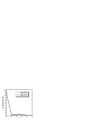
Figure 3: Percentages of regular orbits on the subspace $x_{3}=0.54$, $x_{4}=0.01$ of map (2) for $K=0.5$, as a function of the parameter $B\in[0,2.5]$.

But also GALI₄ can be used for discriminating regular and chaotic motion. From the theoretical predictions for the evolution of GALI₄, we see that after $i=1000$ iterations the value of GALI₄ of a regular orbit should become of the order of $10^{-16}$, since GALI${}_{4}\sim t^{-4}$, although the results of Fig. 1 show that more iterations are needed for this threshold to be reached, due to an initial transient time where GALI₄ does not decrease significantly. On the other hand, for a chaotic orbit GALI₄ has already reached extremely small values at $i=1000$ due to its exponential decay (GALI${}_{4}\sim e^{-4\sigma_{1}i}$). Thus, the global dynamics of the system can be revealed as follows: we follow the evolution of the same orbits as in the case of GALI₂ and register for each orbit the value of GALI₄ after $i=1000$ iterations. All orbits having values of GALI₄ significantly smaller than $10^{-16}$ are characterized as chaotic, while all others are considered as non–chaotic. In the right panel of Fig. 2 we present the outcome of this procedure.

From the results of Fig. 2, we see that both procedures, using GALI₂ or GALI₄ as a chaos indicator, give the same result for the global dynamics of the system, since in both cases 16% of the orbits are characterized as chaotic. These orbits correspond to the black colored areas n both panels of Fig. 2. One important difference between the two procedures is their computational efficiency. Even though GALI₄ requires the computation of four deviation vectors, instead of only two that are needed for the evaluation of GALI₂, using GALI₄ we were able to get a clear dynamical ‘chart’, not only for less iterations of the map (1000 instead of 4000 needed for GALI₂), but also in less CPU time. In particular, for the computation of the data of the left panel of Fig. 2 (using GALI₂) we needed 1 hour of CPU time on an Athlon 64bit, 3.2GHz PC, while for the data of the left panel of the same figure (using GALI₄) only 14 minutes of CPU time were needed.

Using the above–described method, both for GALI₂ and GALI₄, we were able to compute very fast and accurately the percentages of regular motion for several values of parameter $B$. In Fig. 3 we plot the percentage of regular orbits for $B\in[0,2.5]$ where $B$ varies with a step $\delta B=0.1$. We see that the two curves practically coincide, but using GALI₂ we needed almost four times more CPU time. So, it becomes evident that a well–tailored application of GALI_k, with $2<k$, can significantly diminish the CPU time required for the detailed ‘charting’ of phase space regions, compared with that for GALI₂.

References

- (1) Ch. Skokos, T. Bountis and Ch. Antonopoulos, Physica D, 231, 30, (2007).
- (2) H. Kantz and P. Grassberger, J. Phys. A: Math. Gen, 21 L127, (1988).