Three-body interactions in colloidal systems

Abstract

We present the first direct measurement of three-body interactions in a colloidal system comprised of three charged colloidal particles. Two of the particles have been confined by means of a scanned laser tweezers to a line-shaped optical trap where they diffused due to thermal fluctuations. Upon the approach of a third particle, attractive three-body interactions have been observed. The results are in qualitative agreement with additionally performed nonlinear Poissson-Boltzmann calculations, which also allow us to investigate the microionic density distributions in the neighborhood of the interacting colloidal particles.

I Introduction

Pair interactions in dense systems are in general affected by the presence of many other surrounding particles. To take such many-body interactions into account, the degrees of freedom of other particles are often integrated out, leading to effective pair potentials. This concept is often the only way to handle systems where a large number of different length and time scales coexist. It is important to realize, however, that effective potentials - in contrast to true pair potentials - can not be regarded as fundamental quantities because their parameters depend on the state of the system. In addition, no unique way to derive the effective potentials exists and the effective pair potential picture very often leads to thermodynamic inconsistencies Louis . Accordingly, a correct description of any liquid or solid must explicitly take into account many-body effects (and in particular three-body effects as the leading term). Already in 1943 it has been supposed by Axilrod and Teller (AT) Teller and later also by Barker and Henderson Barker that three-body interactions may significantly contribute to the total interaction energy in noble gas systems. This seems to be surprising because noble gas atoms posses a closed-shell electronic structure and are therefore often (and erroneously) regarded as an example of a simple liquid . The conjecture of Axilrod and Teller, however, was confirmed only very recently, when large-scale molecular dynamics simulations for liquid xenon and krypton Bomont ; Jakse was compared with structure factor measurements at small q-vectors performed with small-angle neutron scattering Formisano1 ; Formisano2 . In these papers it has clearly been demonstrated that only a combination of pair-potentials and three-body interactions, the latter in the form of the AT-triple-dipole term Teller , leads to a satisfactory agreement with the experimental data. In the meantime, it has been realized that many-body interactions have to be considered also for nuclear interactions Negele , inter atomic potentials, electron screening in metals Hafner , photo-ionization, island distribution on surfaces Osterlund , and even for the simplest chemical processes in solids Ovchinnikov like breaking or making of a bond.

In view of the general importance of many-body effects it seems surprising that until now no direct measurements of these interactions have been performed. This is largely due to the fact that in atomic systems, positional information is typically provided by structure factors or pair-correlation functions, i.e. in an integrated form. Direct measurements of many-body interactions, however, require direct positional information beyond the level of pair-correlations, which is not accessible in atomic or nuclear systems. In contrast to that, owing to the convenient time and length scales involved, the microscopic information is directly accessible in colloidal suspensions. In addition, the pair-interactions in colloidal suspensions can be varied over large ranges, e.g. from short-ranged steric to long-ranged electrostatic or even dipole-dipole interactions.

In the present study we used charged colloidal particles whose interactions are mediated by the microscopic ions in the electrolyte. The pair interaction in such systems is directly related to the overlap of the ion clouds (double-layers) which form around the individual colloids and whose thickness is determined by the ionic strength of the solution. In highly de-ionized solutions, these double-layers can extend over considerable distances. If more than two colloids are close enough to be within the range of such an extended double layer, many-body interactions are inevitably the consequence. Accordingly, deviations from pair-wise additive interaction energies are expected in charge-stabilized colloidal systems under low salt conditions.

Here we present the first direct measurement of three-body interactions, performed in a suspension of charged colloidal particles. This was achieved by scanned optical tweezers, which provided a trapping potential for two colloidal particles. When a third particle was present, considerable deviations from pair-wise additive particle interactions have been observed. These deviations increased, as the distance of the third particle was decreased and were used to extract three-body interaction potentials. We have additionally performed non-linear Poisson-Boltzmann calculations for the same parameters and same configurations as chosen in the experiment. Deriving the interaction potentials from the solutions of the Poisson-Boltzmann equation, we have correctly taken three-body terms into account. The numerically obtained three-body potentials are in qualitative agreement with the experimental results.

Experimental evidence for many-body interactions has been already obtained from effective pair-interaction potential measurements of two-dimensional (2D) colloidal systems. Upon variation of the particle density, a characteristic dependence of the effective pair interaction was found which has been interpreted in terms of many-body interactions gr . However, during those studies the relative contributions of different many-body terms could not be further resolved. Performing the experiment described in this paper, i.e. observing the system of only three particles, we were able to measure the three-body interactions directly.

II Experimental system

As colloidal particles we used charge-stabilized silica spheres with 990nm diameter suspended in water. A highly diluted suspension was confined in a silica glass cuvette with 200$\mu$m spacing. The cuvette was connected to a closed circuit, to deionize the suspension and thus to increase the interaction range between the spheres. This circuit consisted of the sample cell, an electrical conductivity meter, a vessel of ion exchange resin, a reservoir basin and a peristaltic pump Palberg . Before each measurement the water was pumped through the ion exchanger and typical ionic conductivities below 0.07$\mu$S/cm were obtained. Afterwards a highly diluted colloidal suspension was injected into the cell, which was then disconnected from the circuit during the measurements. This procedure yielded stable and reproducible ionic conditions during the experiments. Due to the ion diffusion into the sample cell, the screening length $\kappa^{-1}$ decreased linearly with time during the measurements. The rate of change of the screening length, however, was only less than half a percent per hour, which means that in the time needed to perform a complete set of measurements, the ionic concentration did not change more than about 1 percent. This tiny variation has been taken into account when performing the PB calculations (see section IV.).

First, three particles were brought in the field of view of the microscope after they had sedimented down to the bottom plate of the sample cell (Fig.1). Two particles were trapped with line-scanned optical tweezers, which was created by the beam of an argon ion laser being deflected by a computer-controlled galvanostatically driven mirror with a frequency of approximately 350Hz. The time averaged intensity along the scanned line was chosen to be Gaussian-distributed with the half-width $\sigma_{x}\approx$ 4.5 $\mu$m. The laser intensity distribution perpendicular to the trap was given by the spot size of the laser focus, which is also Gaussian with $\sigma_{y}\approx$ 0.5 $\mu$m. This yielded an external laser potential acting as a stable quasistatic trap for the particles. Due to the negatively charged silica substrate, the particles also experience a repulsive vertical force, which is balanced by the particle weight and the vertical component of the light force. The potential in the vertical direction is much steeper than the in-plane laser potential, therefore vertical particle fluctuations can be disregarded. The particles were imaged with a long-distance, high numerical aperture microscope objective (magnification $\times$63) onto a CCD camera and the images were stored every 120 ms. The lateral positions of the particle centers were determined with a resolution of about 25 nm by a particle recognition algorithm.

Three-body interaction potentials were measured in this setup by performing the following steps (which will be explained in detail below): First only one particle was inserted into the trap and its position probability distribution was evaluated from the recorded positions. From this the external laser potential $u_{L}$ could be extracted. Next, we inserted two particles in the trap and measured their distance distribution. From this, the pair-interaction potential was obtained. Finally, a third particle was made to approach to the optical trap by means of additional point optical tweezers (focus size $\approx$ 1.3 $\mu$m), which held this particle at a fixed position during the measurement. From the distance distribution of the first two particles we obtained the total interaction potential for the three particles. Finally, we substracted a superposition of pair potentials (known from the previous two-particle measurements) from the total interaction energy to obtain the three-body interaction.

III Data evaluation and experimental results

We first determined the external potential acting on a single particle due to the optical line trap. The probability distribution $P(x,y)$ of finding a particle at the position $(x,y)$ in the trap was evaluated from the recorded positions. $P(x,y)$ depends only on the temperature and the external potential $u_{L}(x,y)$ created by the laser tweezers. According to the Boltzmann probability distribution $P(x,y)=P_{L}\rm{e}^{-\beta u_{L}(x,y)}$, with $P_{L}$ being a normalization constant. Taking the logarithm of $P(x,y)$ yields the external potential $u_{L}(x,y)$ with an offset given by $\log{P_{L}}$. The probability distributions in $x$ and $y$ directions are statistically independent, and can therefore be factorized. The laser potential is thus $u_{L}(x,y)=u_{L}(x)+u_{L}(y)$. The potential along the $x$ axis is shown in Fig.2 for various laser intensities. As can be seen, all renormalized potentials fall, within our experimental resolution, on top of each other. This clearly demonstrates that the optical forces exerted on the particles scale linearly with the input laser intensity. This fact allows us to use different external laser powers for two-body and three-body experiments (in the three-body experiment, due to the additional repulsion of the third particle, a stronger laser power is needed to keep the mean distance between the two particles similar). The corresponding potential in the perpendicular ($y$) direction has the same (Gaussian) shape, but it is much steeper due to the chosen scanning direction. Therefore, the particles hardly move in the $y$ direction during a measurement.

Next, we inserted a second particle in the trap. The four-dimensional probability distribution is now $P(x_{1},y_{1},x_{2},y_{2})=P_{12}\rm{e}^{-\beta\left(u_{L}(x_{1},y_{1})+u_{L}(x_{2},y_{2})+U(r)\right)}$, with $x_{i}$ and $y_{i}$ being the positions of the $i$-th particle relative to the laser potential minimum and $U(r)$ the distance dependent pair-interaction potential between the particles. This can be projected to

$$P(r) = \int\!\!\!\int\!\!\!\int\!\!\!\int P(x_{1},y_{1},x_{2},y_{2})\delta\!\left(\!\sqrt{(x_{1}-x_{2})^{2}+(y_{1}-y_{2})^{2}}-r\right)dx_{1}dx_{2}dy_{1}dy_{2}=$$ (1)

$$= P_{12}\rm{e}^{-\beta U(r)}\!\int\!\!\!\int\!\!\!\int\!\!\!\int\rm{e}^{-\beta\left(u_{L}(x_{1},y_{1})+u_{L}(x_{2},y_{2})\right)}\,\delta\!\left(\!\sqrt{(x_{1}-x_{2})^{2}+(y_{1}-y_{2})^{2}}-r\right)dx_{1}dx_{2}dy_{1}dy_{2}$$

In principle the integral is constituted of all possible configurations of two particles with distance $r$. Performing the full four-dimensional integration, however, is difficult because of the limited experimental statistics. This problem can be overcome by the following two considerations. First, due to the Gaussian shape of the external potential, the most likely particle configurations are symmetric with respect to the potential minimum of $u_{L}$ (any asymmetric configuration for constant $r$ has a higher energy). Secondly, particle displacements in $y$-direction are energetically unfavorable because $\sigma_{x}\gg\sigma_{y}$. Accordingly, for $r=const$ the minimum energy configuration is $(x_{1}=r/2,y_{1}=0,x_{2}=-r/2,y_{2}=0)$. It has been confirmed by a simple calculation with the experimental parameters that all other configurations account for only for less than 1 percent of the value of the integral in Eq.(1). Accordingly, Eq.(1) reduces to

$$P(r)=P_{0}\rm{e}^{-\beta\left(U(r)+2u_{L}(r/2,0)\right)}\;.$$ (2)

Since $u_{L}(x,y)$ is known from the previous one-colloid measurement, we can obtain the interaction potential $U(r)$ from the measured $P(r)$,

$$\beta U(r)\,=\,-\log{P(r)}\,-\,2\beta u_{L}(r/2,0)\,+\,\log{P_{0}}\;.$$ (3)

The normalization constant $P_{0}$ was chosen in a way that $U(r)\to 0$ for large particle separations $r$. We first measured $U(r)$ according to the above procedure in the absence of a third particle. As expected, the negatively charged colloids experience a strong electrostatic repulsion which increases with decreasing distance. The pair-interaction potential of two charged spherical particles in the bulk is well known to be described by a Yukawa potential Landau ; Overbeek

$$\beta U(r)=\beta u_{pair}(r)=\left(Z^{*}\right)^{2}\lambda_{B}\Biggl{(}\frac{\rm{e}^{\kappa R}}{1+\kappa R}\Biggr{)}^{2}\frac{\rm{e}^{-\kappa r}}{r}\;,$$ (4)

where $Z^{*}$ is the renormalized charge Belloni of the particles, $\lambda_{B}$ the Bjerrum-length characterizing the solvent ($\lambda_{B}=e^{2}/4\pi\epsilon\epsilon_{0}k_{B}T$, with $\epsilon$ the dielectric constant of the solvent and $e$ the elementary charge), $\kappa^{-1}$ the Debye screening length (given by the salt concentration in the solution), $R$ the particle radius and $r$ the centre-centre distance of the particles. Fig.3 shows the experimentally determined pair-potential (symbols) together with a fit to Eq.(4) (solid line). As can be seen, our data are well described by Eq.(4). As fitting parameters we obtained $Z^{*}\approx 6500$ electron charges and $\kappa^{-1}\approx 470$nm, respectively. The renormalized charge is in good agreement with the predicted value of the saturated effective charge of our particles Zsat ; Trizac and the screening length agrees reasonably with the bulk salt concentration in our suspension as obtained from the ionic conductivity. Given the additional presence of a charged substrate, it might seem surprising that Eq.(4) describes our data successfully. However, it has been demonstrated experimentally Grier and theoretically Stillinger ; Netz that a Yukawa-potential captures the leading order interaction also for colloids close to a charged wall. A confining wall introduces only a very weak (below 0.1 $k_{B}T$) correction due to additional dipole repulsion. This correction is below our experimental resolution. Repeating the two-body measurements with different laser intensities (50mW to 600mW) yielded within our experimental resolution identical pair potential parameters. This also demonstrates that possible light-induced particle interactions (e.g. optical binding Burns ) are neglegible. The approach of the third particle by means of an additional optical trap could, in principle, lead to additional light-induced interactions between the laser spot and the two particles kept in the line trap. To exclude such effects, we repeated the two-particle measurements and approached an empty trap (without the third particle) to the line trap where the two particles were fluctuating. Within our experimental resolution, we again observed identical pair potentials, which suggests, that the additional optical trap has no influence on the two particles in the line trap. When a third particle is present at a distance $d$ along the perpendicular bisector of the scanned laser line (cf. inset of Fig.1), the total interaction energy $U(r,d)$ is not simply given by the sum of the pair-interaction potentials Eq.(4) alone but also contains an additional term. Following the definition of McMillan and Mayer McM , $U(r,d)$ is given by

$$U(r,d)=u_{pair}(r_{12})+u_{pair}(r_{13})+u_{pair}(r_{23})+u_{123}(r_{12},r_{13},r_{23})\;,$$ (5)

with $u_{pair}(r_{ij})$ being the pair-potential between particles $i$ and $j$ as defined in Eq.(4) and $u_{123}$ the three-body interaction potential. Distances $r_{12}$, $r_{23}$ and $r_{13}$ are the distances between the three particles which can, due to the chosen symmetric configuration ($r_{23}\equiv r_{13}$), be expressed by the two variables $r=r_{12}$ and $d=\sqrt{r_{13}^{2}-(r/2)^{2}}$. We have followed the same procedure as described above for the case of two particles. First, we have measured the probability distribution $P(r;d)$ of the two particles in the laser trap with the third particle fixed at distance $d$ from the trap. Taking the logarithm of $P(r;d)$ we extracted the total interaction energy $U(r,d)$ y-direction . The results are plotted as symbols in Fig.4 for the distance of the third particle $d=4.1,$ 3.1, 2.5 and 1.6 $\mu$m, respectively. As expected, $U(r,d)$ becomes larger as $d$ decreases due to the additional repulsion between the two particles in the trap and the third particle. In order to test whether the interaction potential can be understood in terms of a pure superposition of pair-interactions, we first calculated $U(r,d)$ according to Eq.(5) with $u_{123}\equiv 0$. This was easily achieved because the positions of all three particles were determined during the experiment and the distance-dependent pair-potential is known from the two-particle measurement described above (Fig.3). The results are plotted as dashed lines in Fig.4. Considerable deviations from the experimental data can be observed, in particular at smaller $d$. These deviations can only be explained, if we take three-body interactions into account. Obviously, at the largest distance, i.e. $d=4.1\mu m$ our data are well described by a sum over pair-potentials which is not surprising, since the third particle cannot influence the interaction between the other two, if it is far away from both. In agreement with theoretical predictions Carsten , the three-body interactions therefore decrease with increasing distance $d$.

According to Eq.(5) the three-body interaction potential is simply given by the difference between the measured $U(r,d)$ and the sum of the pair-potentials (i.e. by the difference between the measured data and their corresponding lines in Fig.4). The results are plotted as symbols in Fig.5. It is clearly seen, that in the case of charged colloids $u_{123}$ is entirely attractive and becomes stronger as the third particle approaches. It is also interesting to see that the range of $u_{123}$ is of the same order as the pair-interaction potentials. It might seem surprising that it is possible to sample the potential up to energies of 15$k_{B}T$, as configurations of such a high energy statistically happen only with very low probability. In this experiment we can choose the energetic range of the potential we want to sample by adjusting the strength of the line tweezers. The laser potential pushes the particles together, which allows us to sample different ranges of the electrostatic potential. Thus, to achieve a better resolution for smaller particle separations (e.g. higher potential values), the strength of the line tweezers had to be increased. The shape of the external potential $u_{L}$ was independent of the strength of the laser beam (see Fig.2) and the magnitude scaled linearly with the input laser power. This allowed us to adjust the input laser intensity so as to obtain a suitable particle separation range. The external potential was obtained simply by scaling the Gaussian shown in Fig.2.

IV Numerical calculations

In order to get more information about three-body potentials in colloidal systems, we additionally performed non-linear Poisson-Boltzmann (PB) calculations, in a similar way as in Carsten . The PB theory provides a mean-field description in which the micro-ions in the solvent are treated within a continuum approach, neglecting correlation effects between the micro-ions. It has repeatedly been demonstrated Groot ; Levin that in case of monovalent micro-ions the PB theory provides a reliable description of colloidal interactions. The interactions among colloids are, on this level, mediated by the continuous distribution of the microions and can be obtained once the local electrostatic potential due to the microionic distribution is known. The normalized electrostatic potential $\psi(x,y,z)$, which is the solution of the non-linear PB equation,

$$\mbox{\boldmath$\nabla$}^{2}\psi(\vec{r}) = \kappa^{2}\sinh\psi(\vec{r})\;,$$

$${\bf n}\cdot\mbox{\boldmath$\nabla$}\psi = 4\pi\lambda_{B}\sigma\;,\quad\quad\vec{r}\;\rm{on}\,\rm{colloid}\,\rm{surface}\;,$$ (6)

describes the equilibrium distribution of the microions around a given macroionic configuration. Here $\kappa$ is the inverse Debye screening length , $\lambda_{B}$ the Bjerrum length ($\lambda_{B}=0.72$nm for aqueous solutions at room temperature) and $\sigma$ is the surface charge density on the colloid surface (constant charge boundaries are assumed for all colloids in the system). ${\bf n}$ is the normal unit vector on the colloid surface. We used the multi-centered technique, described and tested in other studies EPL ; JCP to solve the PB equation (6) at fixed configurations of three colloids and obtain the electrostatic potential $\psi(x,y,z)$, which is related to the micro ionic charge density. Integrating the stress tensor, depending on $\psi(x,y,z)$, over a surface enclosing one particle, results in the force acting on this particle. First, we calculated how the force $f_{12}$, and from it the pair-potential between two particles, depend on the distance between isolated two particles. Choosing the suitable bare charge on the colloid surface, we were able to reproduce the measured pair-interaction in Fig.3. The calculation of three-body potentials was then carried out by calculating the total force acting on one particle in the line trap (say, particle 1) in the presence of all three particles and subtracting the corresponding pair-forces $f_{12}$ and $f_{13}$ obtained previously in the two-particle calculation. If there is any difference between the force on particle 1 obtained from the full PB solution for the three particle configuration and the sum of two two-body forces, this difference is due to the three-body interactions in the system. The difference is then integrated to obtain the three-body potential. The results are plotted as dashed and dotted lines in Fig.5 and show qualitative agreement with the experimental data. To account for the deviations from the experimental data one has to take into account the following points: (i) there is a limited experimental accuracy to which the light potential can be determined. The accuracy decreases with increasing laser intensity (note that normalized potentials are plotted in Fig.2). In the three-body experiments, due to the presence of the third repulsive particle, a stronger light field is needed and the experimental error in determining the light potential is estimated to be around $\pm 1k_{B}T$. Since we have to subtract the light potential twice from the total potential to obtain the three-body potential, this error doubles and we expect an error of about $\pm 2k_{B}T$ in the final result. (ii) An error of about $\pm 2k_{B}T$ should be expected in the numerically obtained three-body potentials as well. (iii) While in the numerical calculation we assume identical colloidal spheres, in the experiment small differences with respect to the size and the surface charge are unavoidable. This effect, however, is rather small and leads to deviations on the order of 5 percent of the total potential. (iv) The numerical calculations do not take into account any effects which may be caused by the substrate. Although we expect such effects to be rather small (similar to the contribution for the pair potential) they can not completely ruled out. Considering the above mentioned uncertainties it should be emphasized that in particular the sign and the order of magnitude of the calculated potential compares well with our measured results. This strongly supports our interpretation of the experimental results in terms of the three-body interactions.

We have measured and calculated the three-body interaction on a mesoscopic level, but since the colloidal interactions are mediated by the microions distributed in an electrolyte around the colloids, it is interesting to explore what happens on a microscopic level, i.e., what feature of the microscopic distributions lead to the observed three-body interactions. Of course, it is not possible to observe the microionic density experimentally, but in a Poisson-Boltzmann simulation such an information is easily accessible. Since the microion density depends monotonically on the electrostatic potential $\psi(\vec{r})$, it is enough to compare the electrostatic potentials to qualitatively discuss the microscopic picture. Of course, to a large extent, the potential $\psi(\vec{r})$ around three particles is just the superposition of potentials around individual particles, but since the solutions of nonlinear equations are in principle not superposable, we expect to find small differences. It is indeed these small differences that are ultimately responsible for the three-body interaction.

We started by reconsidering the two-particle problem. First, we solved the PB equation around a single isolated colloid to obtain the one-body non-linear electrostatic potential $\psi^{1}(\vec{r})$. Next we calculated the electrostatic potential $\psi^{2}(\vec{r})$ for two colloidal particles at distance $r$ and compared this potential to the superposition of two one-body potentials $\psi^{1}_{1}(\vec{r})+\psi^{1}_{2}(\vec{r})$. The difference is shown as a contour-plot in Fig.6a. It can be seen that micro-ions are rearranged in a complex way between the colloids. There is a weak additional polarization of the counter-ion cloud very close to the particle surfaces not captured by superposing the one-body potentials. However, all these effects are rather small and therefore, except for very small particle separations r, the superposed solution should still describe the two-body interactions with good accuracy. Not so for three particles. We have compared a superposition of three two-body electrostatic potentials with the correct non-linear three-body electrostatic potential 2b-3b . The difference is shown in Fig.6b. Obviously, differences are now much larger than in Fig.6a. We notice that the counter-ion cloud polarization close to the colloid surface is correctly taken into account by two-body terms, while the ion distribution in the region among the colloids is poorly described by adding up two-body electrostatic potentials. There are fewer counter-ions in the region among the colloids than a pair-wise description predicts. This suggests that the entropy gained by removing some excessive counterions (predicted by the superposition) from the inter-particle space is larger than the positive energy difference due to less efficient screening resulting from it. By integrating the potential difference from Fig.6b, one recovers the attractive three-body potential, already discussed, which is thus demonstrated to be a consequence of the nonlinearity of the physical equations governing the interactions in our system. The exact microscopic explanation of the phenomenon, however, is still lacking and further work is necessary to achieve it.

V Conclusions

We have demonstrated that in case of three colloidal particles, three-body interactions are attractive and of the same range as pair-interactions. They present a considerable contribution to the total interaction energy and must inevitably be taken into account. Whenever dealing with systems comprised of many (i.e. more than three) particles, in principle also higher-order terms have to be considered. The relative weight of such higher-order terms depends on the particle number density $\rho$ . While at low enough $\rho$ a pure pair-wise description should be sufficient, with increasing density first three-body interactions and then higher-order terms come into play. We expect that there is an intermediate density regime, where the macroscopic properties of systems can be successfully described by taking into account only two- and three-body interactions Anti . Indeed liquid rare gases Jakse and the island distribution of adsorbates on crystalline surfaces Osterlund are examples where the thermodynamic properties are correctly captured by a description limited to pair- and three-body interactions attractive-3b . In colloidal systems we have shown the three-body interactions to be comparable in magnitude to the corresponding pair-interactions, therefore we there expect large macroscopic three-body effects in this intermediate density range. At even larger particle densities n-body terms with $n>3$ have to be additionally considered, which may partially compensate. Even in this regime, however, many-body effects are not cancelled, but lead to notable effects, e.g. to a shift of the melting line in colloidal suspensions, as recently demonstrated by PB calculations EPL ; JCP .

With some effort it is in principle possible to proceed to measure the higher order many-body terms and to study how the many-body expansion converges. Work on four-body interactions is in progress.

VI Acknowledgements

Stimulating discussions with R. Klein, C. Russ and E. Trizac are acknowledged. This work has been supported by the Deutsche Forschungsgemeinschaft (Grants Be1788 and Gr1899).

VII Figure captions

Fig.1: Photograph of sample cell with two silica particles confined to a light trap created by an optical tweezers and a third particle trapped in a focused laser beam. The inset shows a schematic drawing of the experimental geometry.

Fig.2: The shape of the laser potential along the tweezers line for three different laser intensities (symbols: triangles 100mW, circles 200mW and squares 500mW); for better comparison all curves are normalized to an intensity of 100mW. The Gaussian fit is plotted as a solid line.

Fig.3: Measured pair-interaction potentials $U(r)=u_{pair}(r)$ (symbols) in the absence of the third particle. The data agree well with a DLVO potential, Eq.(4) (solid line). In the inset the potential is multiplied by $r$ and plotted logarithmically, so that the DLVO expression, Eq.(4) transforms into a straight line. From a fit we obtained the effective charge $Z^{*}\approx 6500$ and the screening length $\kappa^{-1}\approx 470$nm.

Fig.4: Experimentally determined interaction energy $U(r)$ (symbols) for two particles in a line tweezers in the presence of a fixed third particle with distance $d$ on the perpendicular bisector of the line trap. For comparison the superposition of three pair-potentials is plotted as lines. Symbols and lines are labelled by the value of $d$.

Fig.5: Three-body potentials for different $d$. Measured three-body potentials indicated by symbols. The lines are three-body potentials as obtained from the solutions of the nonlinear Poisson-Boltzmann equation for three colloids arranged as in the experiment. The parameters in the Poisson-Boltzmann calculation were chosen so that the pair-interaction potentials were correctly reproduced. Symbols and lines are labeled by the value of $d$.

Fig.6: Contour plots of electrostatic potentials. a) Difference between the full electrostatic potential for two particles and the superposition of two one-particle potentials. The distance between the particles is $r=2.5\mu$m. b) Difference between the full electrostatic potential for three particles and the superposition of three two-particle potentials. The distance between particle 1 and 2 is $r=2.5\mu$m and the position of the third particle is given by $d=1.6\mu$m, being the closest distance realized in the experiments. The colour scales are in units of $k_{B}T$.

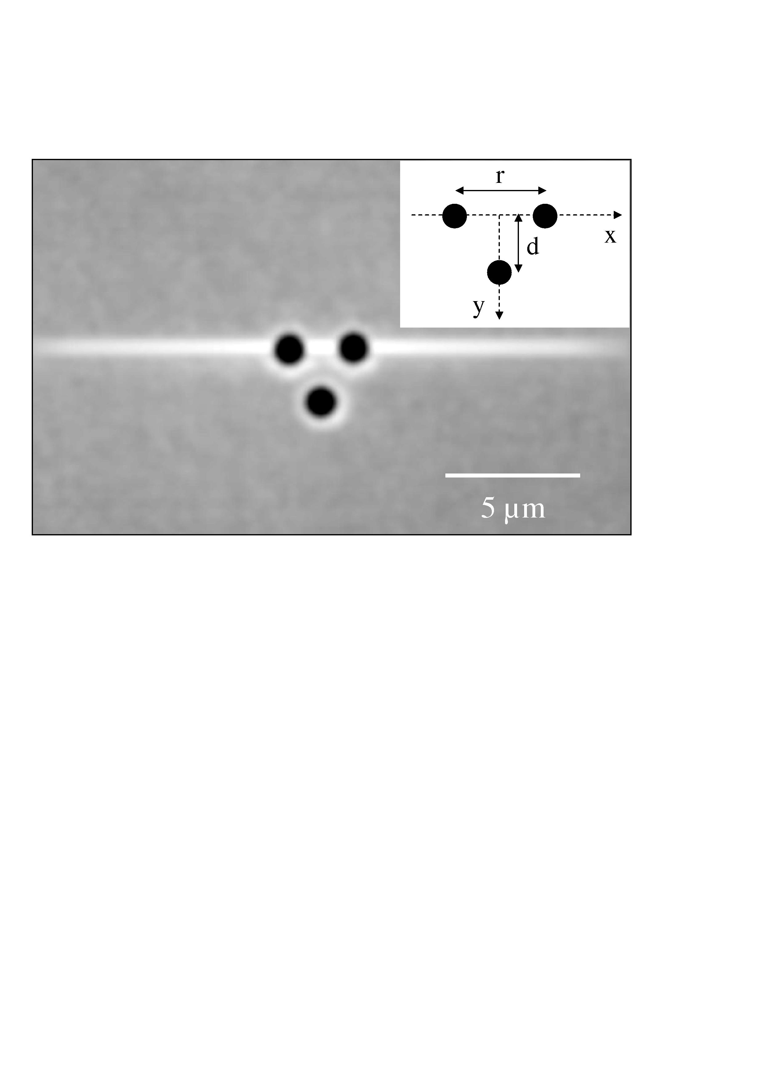
Figure 1:

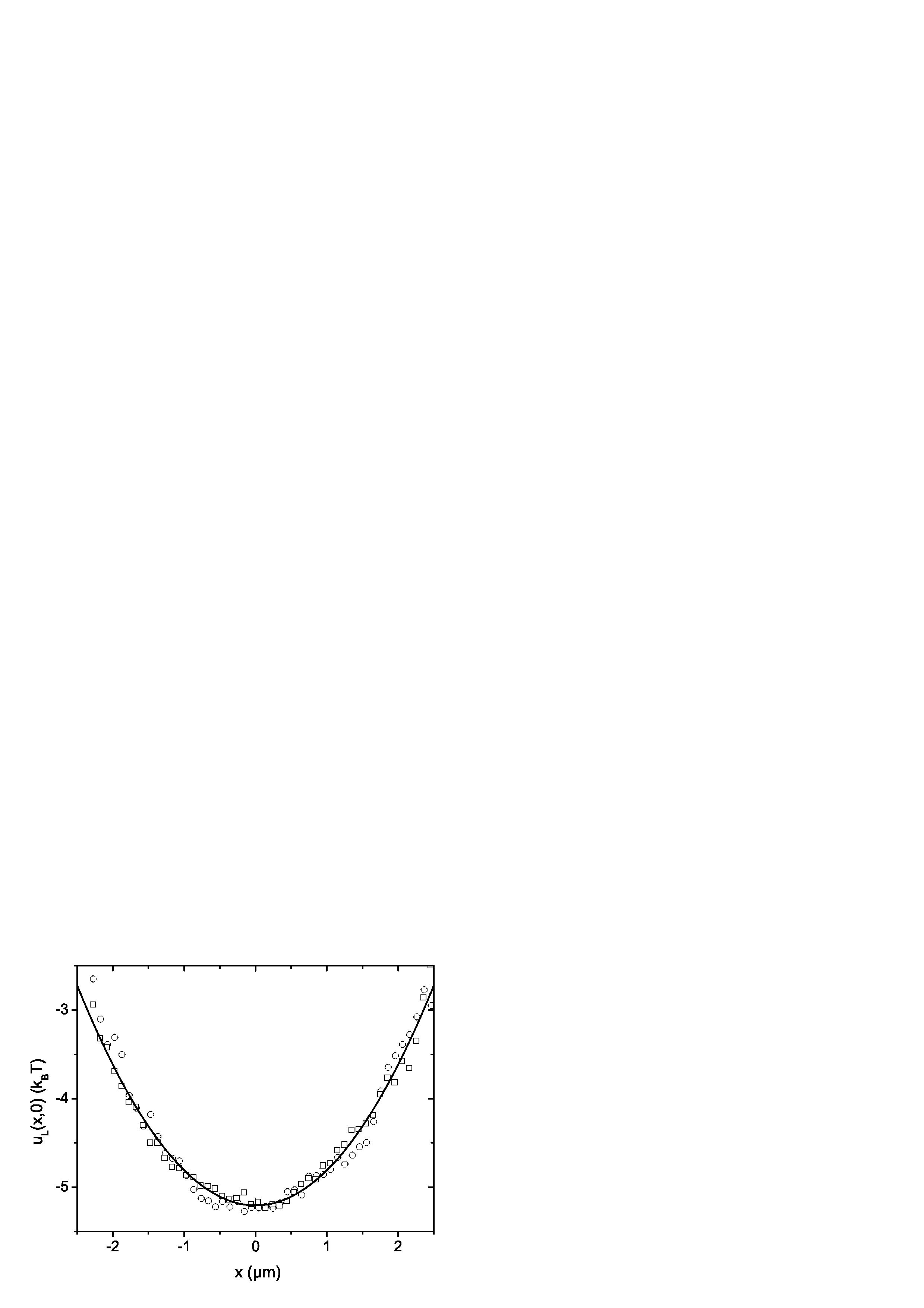
Figure 2:

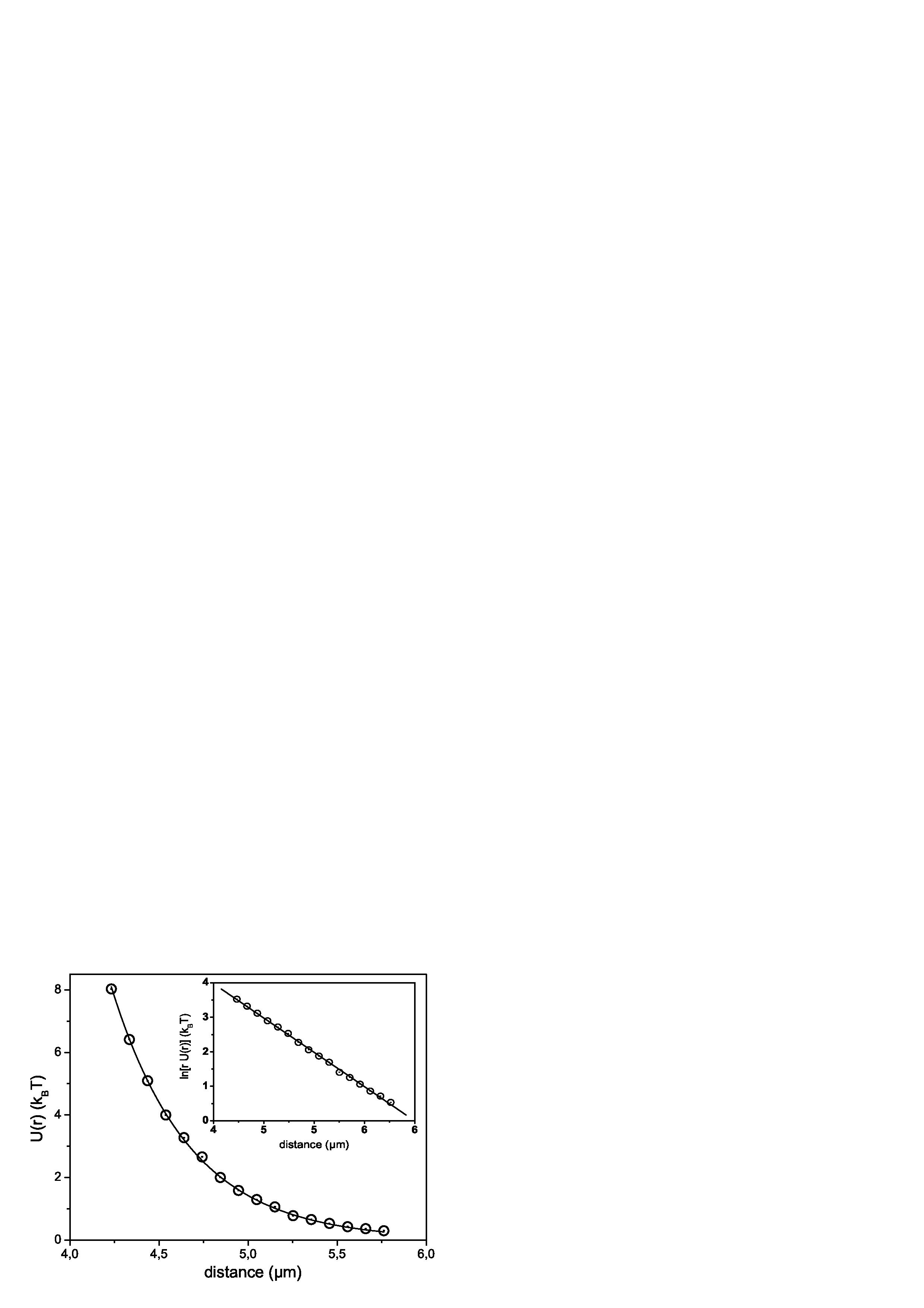
Figure 3:

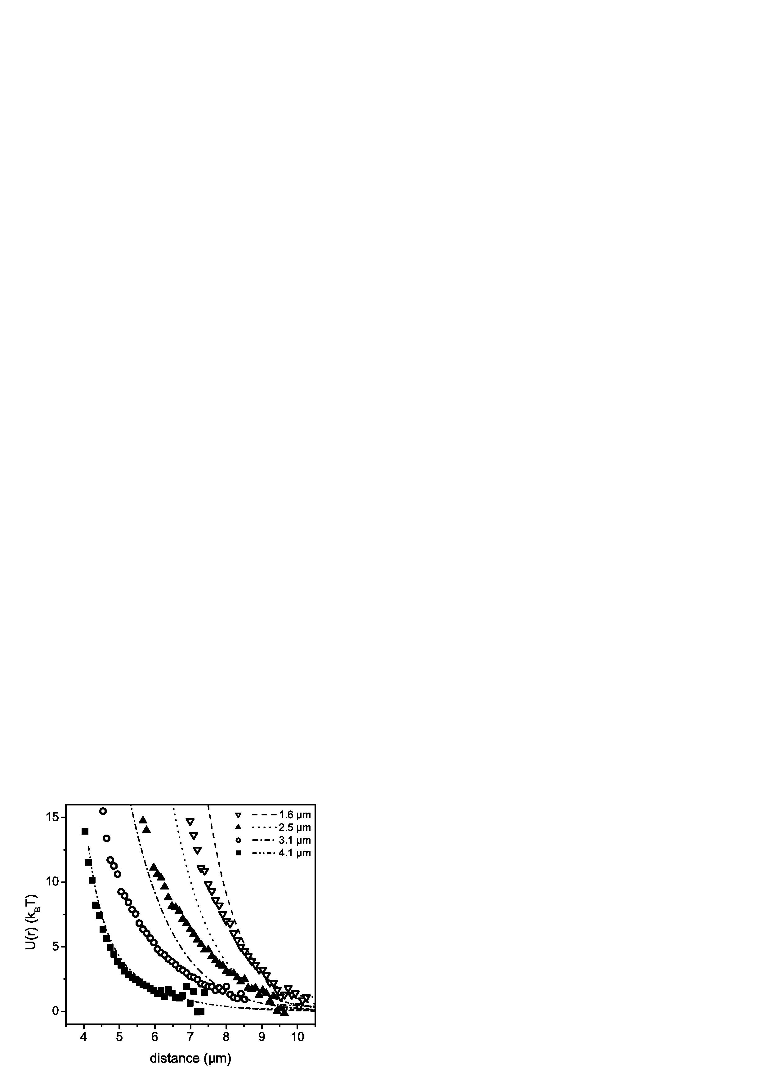
Figure 4:

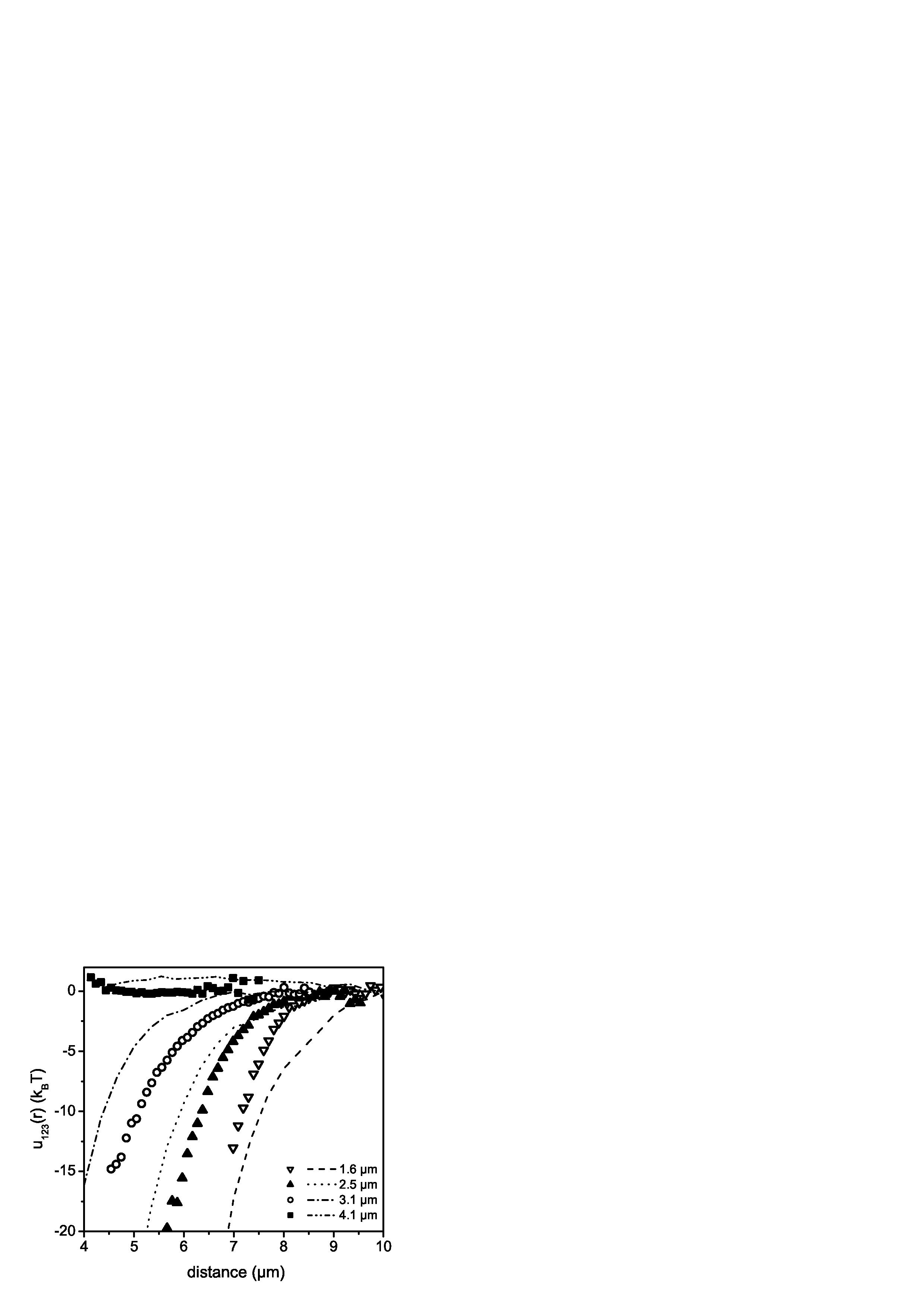
Figure 5:

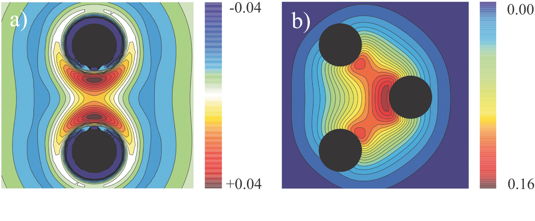
Figure 6:

References

- (1) A. A. Louis, J. Phys.: Condens. Matter 14 (40), 9187 (2002).
- (2) B. M. Axilrod and E. Teller, J. Chem. Phys. 11, 299 (1943).
- (3) J. A. Barker, D. Henderson, Rev. Mod. Phys. 48, 587 (1976).
- (4) J. M. Bomont and J. L. Bretonnet, Phys. Rev. B 65, 224203 (2002).
- (5) N. Jakse, J. M. Bomont, and J. L. Bretonnet, J. Chem. Phys. 116, 8504 (2002).
- (6) F. Formisano, C. J. Benmore, U. Bafile, F. Barocchi, P. A. Egelstaff, R. Magli, and P. Verkerk, Phys. Rev. Lett. 79, 221 (1997).
- (7) F. Formisano, F. Barocchi, and R. Magli, Phys. Rev. E 58, 2648 (1998).
- (8) J. W. Negele, Nucl. Phys. A 669, 18 (2002).
- (9) J. Hafner, From Hamiltonians to phase diagrams (Springer, Berlin, Heidelberg, 1987).
- (10) L. Österlund, M. O. Pedersen, I. Stensgaard, E. Laegsgaard, and F. Besenbacher, Phys. Rev. Lett. 83, 4812 (1999).
- (11) K. Binder and D. P. Landau, Surf. Sci. 108, 503 (1981).
- (12) M. Ovchinnikov and V. A. Apkarian, J. Chem. Phys. 110, 9842 (1999).
- (13) M. Brunner, C. Bechinger, W. Strepp, V. Lobaskin, and H. H. von Grünberg, Europhys. Lett. 58, 926 (2002).
- (14) T. Palberg, W. Härtl, U. Wittig, H. Versmold, M. Würth, and E. Simnacher, J. Phys. Chem. 96, 8180 (1992).
- (15) B. V. Derjaguin and L. Landau, Acta Physicochim U.R.S.S. 14, 633 (1941).
- (16) E. J. W. Vervey and J. T. G. Overbeek, Theory of the stability of lyophobic colloids (Elsevier, Amsterdam, 1948).
- (17) L. Belloni, J. Phys. Cond. Mat. 12, R549 (2000).
- (18) The saturated effective charge of our particles is about 6900 for water at room temperature.
- (19) E. Trizac, J. Phys. A: Math. Gen. 36, 5835 (2003).
- (20) S. H. Behrens and D. G. Grier, Phys. Rev. E 64, 50401 (2001).
- (21) F. H. Stillinger, J. Chem. Phys. 35, 1584 (1961).
- (22) R. R. Netz and H. Orland, Eur. Phys. J. E. 1, 203 (2000).
- (23) M. M. Burns, J. M. Fournier, and J. A. Golovchenko, Phys. Rev. Lett. 63, 1233 (1989).
- (24) W. McMillan and J. Mayer, J. Chem. Phys. 13, 276 (1945).
- (25) When approaching the third particle, the two particles in the trap are slightly displaced in the direction at small . Accordingly, the minimum energy configurations of the two particles are not on a straight line as before. The most likely configuration at given distance is with given by the measured particle positions. Since we have the full knowledge of the two-dimensional external laser potential, we can compute for every given configuration and use it in the Eq.(2) instead of .
- (26) C. Russ, R. van Roij, M. Dijkstra, and H. H. von Grünberg, Phys. Rev. E 66, 011402 (2002). Europhys. Lett. 58, 926 (2002).
- (27) R. D. Groot, J. Chem. Phys. 95, 9191 (1991).
- (28) Y. Levin, Rep. Prog. Phys. 65, 1577 (2002).
- (29) J. Dobnikar, R. Rzehak, and H. H. von Grünberg, Europhys. Lett. 61, 695 (2003).
- (30) J. Dobnikar, Y. Chen, R. Rzehak, and H. H. von Grünberg, J. Chem. Phys. 119 (9) (2003).
- (31) In the configuration of three particles we have three pairs. We have first performed three Poisson-Boltzmann calculations with two particles (each pair isolated) to obtain the two-body electrostatic potentials . We superposed those three solutions to obtain a prediction for the electrostatic potential around three particles without taking three-body effects into account. Then we performed the Poisson-Boltzmann calculation around three particles to obtain the correct electrostatic potential . The difference is plotted on Fig.6b and this is the microscopic origin of the measured three-body interaction .
- (32) A.-P. Hynninen, M. Dijkstra and R. van Roij, J. Phys. Cond. Mat. 15 (48), S3549 (2003).
- (33) Three-body interactions are not always attractive. In case of van der Waals interactions, the AT-triple dipole interactions are predicted to be either positive or negative, depending on the configuration of the particles.