Many-body interactions and melting of colloidal crystals

Abstract

We study the melting behavior of charged colloidal crystals, using a simulation technique that combines a continuous mean-field Poisson-Boltzmann description for the microscopic electrolyte ions with a Brownian-dynamics simulation for the mesoscopic colloids. This technique ensures that many-body interactions between the colloids are fully taken into account, and thus allows us to investigate how many-body interactions affect the solid-liquid phase behavior of charged colloids. Using the Lindemann criterion, we determine the melting line in a phase-diagram spanned by the colloidal charge and the salt concentration. We compare our results to predictions based on the established description of colloidal suspensions in terms of pairwise additive Yukawa potentials, and find good agreement at high-salt, but not at low-salt concentration. Analyzing the effective pair-interaction between two colloids in a crystalline environment, we demonstrate that the difference in the melting behavior observed at low salt is due to many-body interactions. If the salt concentration is high, we find configuration-independent pair-forces of perfect Yukawa form with effective charges and screening constants that are in good agreement with well-established theories. At low added salt, however, the pair-forces are Yukawa-like only at short distances with effective parameters that depend on the analyzed colloidal configuration. At larger distances, in contrast, the pair-forces decay to zero much faster than they would following a Yukawa force law. This is explained with a screening effect of the macroions. Based on these findings, we suggest a simple model potential for colloids in suspension which has the form of a Yukawa potential, truncated after the first coordination shell of a colloid in a crystal. Using this potential in a one-component simulation, we find a melting line that shows good agreement with the one derived from the full Poisson-Boltzmann-Brownian-dynamics simulation.

I Introduction

The classic Derjaguin-Landau-Verwey-Overbeek (DLVO) theory verwey ; likos01 ; levin02 ; reviewBelloni00 ; rev:attard ; rev:loewen predicts that an isolated pair of charged colloidal spheres in an aqueous salt solution interacts via a repulsive Yukawa potential at large separations, a prediction that has recently been confirmed by direct experimental measurements crocker352 ; vondermasson1351 ; crocker1897 . However, in nature colloidal particles usually do not occur simply as pairs, but rather in form of suspensions. Then the DLVO pair potential does not always provide a valid description of the intercolloidal interactions as becomes clear from the following considerations. The DLVO potential is an effective colloid-colloid potential, obtained after integrating out the microionic degrees of freedom; it is governed by the density distribution of the ionic fluid between two interacting colloids. However, when more than two colloids are present, as it is the case in colloidal suspensions, then this density distribution can be sensitively influenced by other colloids in the neighborhood, i.e., by both the presence of the fixed charges on the colloidal surfaces and the exclusion of electrolytic solution from the volume occupied by the colloid. Because of these confinement and polarization effects, colloidal interactions in suspensions in principle are non-additive, that is, the total potential energy can not be written as a sum of simple pair-interactions.

The implications of this interesting many-body aspect of charge-stabilized colloidal suspensions have been addressed by various authors. Linse linse91 studied asymmetric two-component electrolytes (charge asymmetry 1:20) within the primitive model and explored pair- and triplet-correlations among colloidal particles in concentrated suspensions. He compared his data with the results of a simulation of an effective one-component system, consisting only of colloids interacting via effective pair-potentials, chosen such that the pair-correlations in the original two-component system and in the reference one-component system are identical. Although in general rather similar triplet correlation functions were obtained, considerable differences became visible at small distances, pointing to the existence of many-body forces. In a more direct way, three-body forces have been analyzed by Löwen and Allahyarov allah using primitive model simulations in a triangular geometry of colloids. Interestingly enough, these three-body forces are attractive, representing a substantial correction to the repulsive pair-forces, a finding that has been corroborated by recent primitive model wu and Poisson-Boltzmann simulations russ , see also tehver1335 .

The present work addresses the question how three- and higher-order body forces affect the melting behavior of colloidal crystals. Starting from crystalline configurations, we compute the mean-square displacement of colloids about their lattice site and use Lindemann’s rule to estimate the solid-liquid phase-boundaries. The simulation technique we use, has been suggested by Fushiki fushiki6700 ; it combines a Poisson-Boltzmann field description for the microions with a Brownian dynamics simulation for the macroionic colloids, an approach which ensures that many-body interactions between the colloids are fully included. In order to identify many-body effects we have to contrast the phase-diagram resulting from these simulations to the predictions based on the established description of colloidal suspensions in terms of pairwise Yukawa potentials. This requires a procedure by which we can map our original many-body non-linear system onto an effective linear pairwise additive Yukawa system. This is done here by calculating effective pair-forces between colloids which are then fitted to Yukawa pair-potentials. Our main result is that the melting line of a colloidal system with purely pair-wise additive potentials is shifted towards the crystalline side of the phase-diagram if many-body forces are added. In view of the fact that three-body forces are already known to be attractive, this result is what one would expect: for a colloidal crystal whose stability results from repulsive pair-forces, adding attractive triplet forces should have a destabilizing effect on the crystal so that it melts earlier than it would without these three-body forces. We will however see that it is not straightforward to spot the many-body forces as being responsible for this effect.

After some general remarks in sec. II on many body interactions in colloidal systems, we will give in sec. III a description of the system and the simulation methods used. Sec. IV is then devoted to a presentation of our effective force calculations in colloidal FCC and BCC crystals, followed by sec. V in which we will discuss the phase behavior of a Yukawa system. This, together with the results from sec. IV, will enable us to compare in sec. VI the melting behavior resulting from our simulations with that of a simple Yukawa system. Sec. VII contains a summary of our results and the general conclusion.

II Many-body interactions and density-dependent pair-potentials in colloidal systems

There exists a bijective one-to-one mapping between a unique pair potential $u_{\mathrm{eff}}(r,\rho)$ and the pair correlation function $g(r)$ at the density $\rho$ henderson74 . That is, even in systems where the true interaction potential contains a strong three-body contribution $u_{3}(r_{12},r_{13},r_{23})$, one can interpret the pair correlation function in terms of (now effective) pair-potentials $u_{\mathrm{eff}}(r,\rho)$. These effective potentials are to be distinguished from the true pair-potential $u(r)$. To lowest order in $\rho$, $u_{\mathrm{eff}}(r,\rho)$ reads attard92 ; reatto87 ; ram77

$$\beta u_{\mathrm{eff}}(r)=\beta u(r)-\rho\!\int\!g_{0}(r_{13})g_{0}(r_{23})(e^{-\beta u_{3}(r_{12},r_{13},r_{23})}-1)\,d{\bm{r}}_{3}\;,$$ (1)

where $\beta=1/k_{B}T$ and where $g_{0}(r)$ is that radial distribution function which is based on the true pair potential $u(r)$ alone. Eq. (1) states in essence that the three-body interactions can be integrated out, and that the resulting effective pair-potential becomes state-dependent. In other words, taking eq. (1) as a model pair-potential in a system with pair-wise interactions only, one can, at low density, calculate the correct pair-correlation function for the true system, consisting of particles interacting via $u(r)$ and $u_{3}(r_{12},r_{13},r_{23})$.

Eq. (1) is the key to an understanding of a recent experiment in 2D suspensions of charged colloids klein ; brunner which being intimately related to the subject of this paper, we briefly summarize in the following. In this experiment digital video microscopy has been used to systematically investigate the effective pair-potentials $u_{\mathrm{eff}}(r,\rho)$ as a function of the colloid densities $\rho$. At relatively low densities, potentials very close to Yukawa form have been observed, just as standard DLVO theory predicts. For increasing density, however, the measured potentials were Yukawa-like only at very short distances but showed clear and systematic deviations from the Yukawa form at larger distances. From eq. (1) it is seen that a density-dependence of $u_{\mathrm{eff}}(r,\rho)$ reveals the existence of many-body interactions, in particular three-body interactions. According to allah ; wu ; russ three-body forces between charged colloids are attractive, so $u_{\mathrm{eff}}(r)$ in eq. (1) should be smaller than $u(r)$ in the distance regime where $u_{3}(r_{12},r_{13},r_{23})$ is appreciable. This has indeed been observed in klein ; brunner . Another observation made in this experiment has been that the radial distance where the measured $u_{\mathrm{eff}}(r,\rho)$ started to show deviations from $u(r)$ was correlated with the mean colloid-colloid distance $d_{m}=\rho^{-1/2}$ (in 2D).

These observations show that three-body interactions between the colloids in the suspension are non-negligible and that they indeed seem to be attractive as predicted in allah ; wu ; russ . A clearer idea of the experimental findings is given by the following interpretation: two colloids, A and B, separated by a distance $r<d_{m}$, will behave as if they were in isolation, i.e. the interaction is determined solely by the microions and the pair-potential is Yukawa-like. However, if $r\geq d_{m}$, then it is very likely that there is a third colloidal particle, C, near the line joining the two interacting colloids A and B. This third particle has a threefold effect on the interaction between the particles A and B. First, there is a confinement effect; the electrolyte solution is excluded from the volume occupied by particle C. Secondly, colloids are usually made of materials that have a much lower dielectric constant than that of the aqueous solvent; electric field lines will then also be excluded from the volume of particle C. And, finally, the colloids are charged; thus the charges of particle C will affect the microionic charge distribution between the two interacting colloids A and B. All three effects result in a pair-interaction between A and B that will depend on the position of particle C. This can be taken into account by choosing a description either in terms of density-dependent effective pair-potentials or in terms of density-independent pair-potentials plus many-body interactions. The effect of particle C on the interaction between A and B is the stronger the nearer C is to the joining line between A and B, and certainly strongest, if C lies directly on this line. In russ , this coaxial geometry has been considered, and it has been found that the three-body potential equals a considerable fraction (up to 90% for almost touching colloidal spheres) of the negative of the pair-potential between the two outer particles (particle A and B). This means that the middle colloid essentially shields (or ”screens”) the two outer ones from each other; it blocks the direct (repulsive) pair interaction between them. In other words, the triplet interaction describes, to lowest order, the screening of pair interactions due to additional macroions. One may say that the interaction between two colloids at large distances ($r\geq d_{m}$) is screened by both microions and macroions, while it is screened just by the microions if $r<d_{m}$; so the effective $\kappa$ in the former case is larger than in the latter case because the ionic strength is higher when macro- and microions are counted in comparison to the case where only the microions are taken into account warren . Because the screening mechanism involving macro- and microions is much more efficient, the pair interaction between colloids in suspension will decay much faster than the interaction between an isolated pair of colloids.

In fact, it is just this cross-over from a microion-dominated to a macroion-dominated screening that has been observed in the experiment in klein ; brunner , and the distance where this happens was indeed roughly given by $d_{m}$, beyond which value the effective pair-potentials decayed so rapidly to zero, as if they were cut off. Such a ”cut-off” like behavior, caused by macroion screening, is also found in the effective force curves we present in Sec. IV. It also plays a decisive role when in Sec. V we try to understand the solid-liquid phase behavior of colloidal suspensions with truncated and density-dependent effective pair-potentials, chosen to model the effect of many-body interactions.

In rare-gas systems it has long been known that a description in terms of pair-potentials is not strictly valid because the interaction between two particles is again disturbed by the presence of a close third particle henderson76 . In these systems, one usually describes the interaction between the atoms by combining a pair-potential with the so-called Axilrod-Teller triple-dipole potential axilrod43 . Mainly the effect of this additional many-body potential on the pair-correlations functions has been studied for krypton tau89 ; jakse02 , argon barker71 ; bukowski01 and xenon bomont02 . Most of these papers are large-scale computer simulations, including the classic work of Barker et al. barker71 , others present perturbation ram77 and integral-equation theories attard92 ; bomont02 in which the pair-correlation functions is calculated from the Ornstein-Zernike equation using a closure that involves the effective pair-potential from eq. (1). Concerning the gas-liquid equilibrium, the effect of the Axilrod-Teller interaction potential has been studied for argon in bukowski01 , where only a moderate difference to the pairwise interactive case was found.

Contrary to these rare-gas fluids, where one is simply stuck with the interaction dictated by the electronic structure of the atoms, the interactions between charged colloidal particles can be adjusted by adding salt to the electrolyte. Specifically, three-body interactions between the colloids can be ’switched-off’ just by adding salt. This allows to investigate experimentally how the behavior of a suspension of charged colloids depends on their interactions. The possibility of tuning the interactions in an experiment makes colloidal suspensions a system that is ideally suited for studying many-body effects.

The salt concentration thus is an important quantity in the following discussion. It is best specified by means of the inverse Debye screening length $\kappa^{-1}$. This is also a natural measure for the interaction range of effective colloidal interactions, as it gives the thickness of the spherical double-layer around a single isolated colloidal sphere. Comparing $\kappa^{-1}$ to the mean colloid-colloid distance $d_{m}$, we can estimate when we expect three-body interactions to be important. If two spherical double-layers overlap, the screening of the colloidal charges becomes incomplete and the charge distributions on the colloids involved begin to interact. If the colloid density is low, i.e. if $d_{m}\kappa\gg 1$, it is obvious that such an overlap will almost always occur for pairs of colloids only. At high colloid densities, however, i.e. if $d_{m}\kappa\sim 1$, there is a high probability that more than one other colloid is within the range of the double-layer $\kappa^{-1}$ around any colloidal particle. Many-body forces between the colloids thus become important under low-salt conditions and/or at high colloid densities warren .

Unlike in rare-gas systems, the effect of triplet interactions allah ; wu ; russ ; tehver1335 on the phase-behavior of charged colloids has not received much attention. Wu et al. wu have used their simulated three-body potentials to calculate the densities of the coexisting phases by simple van-der-Waals theories for the solutions and the colloidal crystals. They studied colloidal systems in monovalent electrolyte solutions, with and without triplet forces, and found only small differences. However, they investigated systems at rather high salt concentrations ($0.05$ M) while as pointed out above, the physics of charged colloidal suspensions becomes special only at low-added salt beresfordsmith . The interesting features of phase equilibria in charged colloidal suspensions at low-salt conditions have also been pointed out in vanroij99 . Linse et al., in a series of papers linse91 ; linse4359 ; linse4208 ; linse3917 , have explored by primitive model simulations the structure, phase-behavior and thermodynamics of a model system consisting of charged colloids and point counterions (with up to 80 counterions per colloid); these authors concentrated mainly on a possible gas-liquid phase-coexistence, but not on the crystallization behavior of their system.

The considerations made above show that in the presence of many-body interactions, the effective pair-potential becomes density-dependent. That a density-dependence of the pair-potential can produce a van-der-Waals like instability even in fluids with purely repulsive pair potentials has been shown for a colloidal system by Dijkstra et al.dijkstra1219 . It can also lead to a second liquid-liquid phase separation in systems that already show a gas-liquid phase-coexistence almarza2038 . A broad discussion of density-dependent pair-potentials with many illustrative examples of typical soft-matter systems is given by Louis louis02 , including recent theoretical studies of coarse graining of polymers as ’soft colloids’ louis00 ; bolhuis01 . Louis points out that the effective density-dependent pair potential in eq. (1), though reproducing the correct pair-structure, will not generate the correct virial pressure. The implications of this inconsistency for the thermodynamics of the fluid is considered in tejero02 . This shows the importance of investigations like ours taking full account of the many-body nature of colloidal interactions.

III Simulation technique

We now give a short description of the technique we have used to calculate effective forces in sec. IV and the melting line of colloidal crystals in sec. VI. More details about our simulation method can be found in technical_paper .

We consider a fluid of highly charged identical colloidal spheres suspended in a structureless medium of dielectric constant $\varepsilon$ at temperature $T$. The Bjerrum length characterizing the medium is defined as $\lambda_{B}=e^{2}\beta/\varepsilon$, with $e$ the elementary charge. The colloidal spheres have radius $a$, charge $-Ze$, and thus a surface charge density $-e\sigma=-Ze/4\pi a^{2}$. The positions of their centers are denoted by ${\bf R}_{i}$ ($i=1\ldots N)$. The suspension is assumed to be in osmotic equilibrium with an electroneutral and infinite reservoir of monovalent point-like salt ions with total particle density $2c_{s}$ and inverse Debye screening length $\kappa=(8\pi\lambda_{B}c_{s})^{1/2}$, and also in thermal equilibrium with a heat bath at constant temperature. In the Poisson-Boltzmann (PB) mean-field approach, the density distribution of the positive and negative microions in the region $G$ exterior to the colloidal spheres at $\{{\bf R}_{i}\}$ is given by $n_{\pm}=c_{s}e^{\mp\phi({\bm{r}})}$ where $\phi({\bm{r}})$ is the normalized electrostatic potential satisfying the PB equation

$$\begin{array}[]{rclcl}\mbox{\boldmath$\nabla$}^{2}\phi({\bm{r}})&=&\kappa^{2}\sinh\phi({\bm{r}})\>,&&{\bm{r}}\in G\\ {\bf n}_{i}\mbox{\boldmath$\nabla$}\phi&=&4\pi\lambda_{B}\sigma&&{\bm{r}}\in\partial G_{i},\>i=1,\ldots,N\>,\end{array}$$ (2)

with $\partial G_{i}$ being the surface of the $i$-th colloid with outward pointing surface normal ${\bf n}_{i}$. Constant-charge boundary conditions are assumed for all $N$ colloid surfaces.

Eq. (2) is based on a description in the semi-grand-canonical ensemble. The suspension is assumed to be separated from the reservoir by a semi-permeable membrane, through which solvent molecules and microions can pass, but not colloidal particles. This leads to an imbalance in the osmotic pressure across the membrane. The equilibrium between the suspension and the salt reservoir is referred to as Donnan equilibrium Don24 ; Ove56 ; hill56 . The effective average salt concentration $n_{s}$ in the suspension is not the same as the reservoir salt concentration $c_{s}$, but is a function of the physical parameters of the system and can be calculated, e.g., in the PB cell model reus97 ; TaLe98 ; deserno . Here, we can compute $n_{s}$ from the total number of microions, obtained by integrating the microionic density distribution, $n_{+}({\bm{r}})+n_{-}({\bm{r}})$, over $G$. Since the actual salt concentration in the system, $n_{s}$, is of no interest in the following considerations we dispense with quantifying it, but will instead specify just $c_{s}$, or, equivalently, $\kappa a=(8\pi(\lambda_{B}/a)c_{s}a^{3})^{1/2}$ which for simplicity we will refer to as ’salt concentration’.

In many experiments, the system is actually not coupled to a salt reservoir and only $n_{s}$ is known. One can then imagine it to be coupled to a (physically not existing) reservoir with a salt concentration $c_{s}$ chosen such that it corresponds to the given $n_{s}$ in the system. Practically, this amounts to inverting the function $n_{s}(c_{s})$. Provided we only choose the right $c_{s}$ corresponding to the known $n_{s}$, a real reservoir when coupled to the system would leave the microion density distribution in the system completely unaltered. In other words, every system, be it isolated or not, can be treated as if it were in contact with a reservoir. This implies that all our considerations presented here in the semi-grand canonical ensemble are also valid for experiments in the canonical ensemble in which the system is actually not coupled to a salt reservoir.

The PB equation rev:andel can be derived from a mean-field free energy functional Lev39 ; BrRo73 ; ReRa90 ; trizac97 ; rev:deserno ; tama02 which itself is obtained from the underlying Hamiltonian either (i) as the saddle point of the field theoretic action PoZe88 ; CoDu92 ; netz00 ; BoAn00 , (ii) as a density functional reformulation of the partition function combined with a first order cumulant expansion of the correlation term lhm , or (iii) from the Gibbs-Bogoljubov inequality applied to a trial product state rev:deserno . The PB approximation gives a good description in the limit of high temperature and/or small charge densities (weak-coupling limit) when the microionic correlations that are neglected at the mean-field level are unimportant. Indeed, these microion correlations play only a negligible role in our system containing only monovalent ions, as has been shown in various studies groot ; valleau ; lhm ; lobaskin99 ; lobaskin01 . Groot groot , for example, quantified the validity of the PB approach by comparing it to a cell model Monte-Carlo simulation and showed that the deviations are already tiny for a ratio $\lambda_{B}/a=0.03$. Since we are here considering an even smaller value $\lambda_{B}/a=0.012$, the PB approach is perfectly justified.

To simulate now the dynamics of the large macroions suspended in the microionic liquid, the PB field description of the small ions in eq. (2) is combined with a Brownian dynamics simulation of the macroions, similar to Refs. fushiki6700 ; gilson95 . For each spatial configuration of the macroions, the electrostatic potential $\phi$ arising from all charges in the system is determined by solving eq. (2) with boundary conditions determined by the positions of the macroions and the charges on them. To truncate the ideally infinite suspension volume with a minimum of finite size effects, a cubic simulation box with periodic boundary conditions on its faces is considered. From the electrostatic potential, the force ${\bf F}^{\phi}_{i}$ acting on each of the macroions is calculated by integrating the normal component of the stress tensor

$$\beta{\mathsf{T}}=\frac{1}{8\pi\lambda_{B}}\bigg{(}\Big{(}2\kappa^{2}\left(\cosh\phi-1\right)+\left(\mbox{\boldmath$\nabla$}\phi\right)^{2}\Big{)}{\mathsf{1}}-2\mbox{\boldmath$\nabla$}\phi\otimes\mbox{\boldmath$\nabla$}\phi\bigg{)}$$ (3)

over a surface enclosing the respective macroion. These forces are then used to perform one time step in a Brownian dynamics simulation for the motion of the macroions, generating another colloidal configuration for the next iteration cycle.

For large colloidal charge $Z$, the solution of the PB equation may develop rather steep boundary layers close to the particle surfaces while far away it varies only gradually. To provide an accurate resolution of the boundary layers with a reasonable number of grid points, we follow Ref. fushiki6700 and define a spherical grid in a shell centered about each of the macroions overset on a Cartesian grid covering the simulation box. The resolution near the particle surfaces is further enhanced by choosing the radial spacing of spherical grid points such that the inverse radial coordinate has a constant increment muller28 . The solution of the PB equation on the domain $G$ outside the macroions is then obtained in four steps: First the PB equation is solved in each of the $N$ spherical shells $\Omega_{1},\ldots,\Omega_{N}$ assuming given potential values at their outer edges. Interpolation of these spherical shell solutions to the Cartesian grid next yields boundary values for the interstitial region $\Omega_{0}$ which is the part of the domain $G$ not contained in any of the spherical shells. With these boundary values the PB equation is then solved in the interstitial region. Finally, new boundary values on the outer edges of the spherical shells are found by interpolating back from the interstitial solution. These steps are repeated until a converged solution on the whole domain $G$ is obtained.

The PB equation is discretized by a finite volume procedure fletcher91 to handle the singular points on the polar axis of the spherical grids. For the non-singular grid points of the spherical and Cartesian grids this reduces to a simple second order finite difference method. On each of the grids the discretized PB equation is solved by a nonlinear ’Successive Over-Relaxation’ (SOR) method ortega70 . The iteration is terminated when the maximum of the absolute value of the residuum for all grid points drops below some desired accuracy. Note that it is not necessary to iterate to convergence in each of the repeatedly solved sub-domain problems for $\Omega_{0},\ldots,\Omega_{N}$. Only in the last pass of this repetition, the full convergence must be ensured.

The integration of the normal component of the stress tensor that gives the force on the macroions turns out to be best performed in the middle of the spherical shell $\Omega_{p}$ around each particle. The derivatives of the electrostatic potential appearing in the stress tensor are discretized by central differences while the midpoint rule is used to approximate the surface integral.

The equation of motion for the macroions reads

$$\zeta\dot{\bf R}_{i}={\bf F}^{\phi}_{i}+\sqrt{2k_{\rm B}T\>\zeta\,}\>\mbox{\boldmath$\xi$}_{i}\;,$$ (4)

where $\zeta=6\pi\eta a$ is the Stokes friction coefficient of a macroion in the solvent of viscosity $\eta$, and where $\vec{{\xi}}_{i}$ is an uncorrelated Gaussian white noise with zero mean and unit variance. This equation is advanced in time by a stochastic Euler algorithm kloeden92 ; oettinger96 with time step $h$. A time-discrete approximation to the white noise $\vec{\xi}_{i}$ is furnished by a sequence of random numbers with zero mean and variance $h$ drawn independently at each time step. Since we are interested only in calculating averages from the trajectories, only the first two moments of the distribution of these random numbers are important kloeden92 ; oettinger96 .

This method allows to calculate structural and thermodynamic properties of charge-stabilized colloidal suspensions in the parameter regime of large macroionic charge, low salt concentration, and relatively high colloid volume fraction, where many-body interactions between the macroions become important. By describing the small ions in terms of a continuous density, the computational effort becomes independent of their number. In this way, the main limitation, which precludes the application of primitive model simulations to the above parameter regime is circumvented. At the same time, in contrast to analytical treatments like linearized DLVO theory or cell models, macroionic many-body effects are fully accounted for in our approach.

There are a few studies loewen673 ; lhm ; tehver1335 ; fushiki6700 where similar simulations have been carried out. The method used by Löwen et al. lhm ; loewen673 is based on a density functional approach which includes also a LDA micro-ion correlation term; it becomes equivalent to the method we used, if one neglects the microion-microion correlations. The technically most difficult part of these simulations are the numerical solution of the boundary-value problem in eq. (2) for arbitrary $\{{\bf R}_{i}\}$ which is solved in different ways in lhm ; loewen673 ; tehver1335 and fushiki6700 . The overset-grid technique we here use following fushiki6700 , is more accurate for a comparable number of grid points than the single grid computations used in lhm ; loewen673 ; tehver1335 , and thus allows to consider more highly charged colloids. Löwen et al. lhm and Fushiki fushiki6700 , both working in the salt-free case, used this method to calculate structure functions and pair distribution functions of colloidal dispersions in the fluid phase, compared with MC simulations, and predictions of the DLVO theory and the PB cell model alexander . Mapping many-body interactions onto optimal Yukawa pair-interactions is the key idea of loewen673 , considering, as in the present paper, colloidal systems with added salt.

We have four different length scales in the system which are: the screening length $\kappa^{-1}$, the colloidal hard-sphere radius $a$, the Bjerrum length $\lambda_{B}$, characterizing the solvent, and the mean-distance $d_{m}=\rho^{-1/3}$ (in 3D) between the colloids in a suspension at a number density $\rho$ (volume fraction $\eta=4\pi\rho a^{3}/3$). A further physical parameter of our system is the colloidal charge $Z$. Taking (i) the radius $a$ of the colloidal spheres as unit-length scale and concentrating (ii) on colloid particles of a typical size of $a=60$nm common in experimental studies gast89 ; yama5806 in aqueous systems at room temperature where $\lambda_{B}=7.2\>\AA$, we fix the ratio $\lambda_{B}/a=0.012$, a value which is used throughout this work. The state space of our colloidal system is thus three-dimensional, spanned by $\kappa a$ (salt concentration), $Z$ (colloidal charge) and $d_{\mathrm{m}}/a$ (colloid density), or, equivalently, the volume-fraction $\eta=4\pi(a/d_{\mathrm{m}})^{3}/3$. A point $\vec{X}$ in state space is then defined by $\vec{X}\equiv(\kappa a,Z,\eta)$. Since a systematic exploration of the full 3D state space is computationally too expensive, we here focus on a 2D cut at large volume fractions and take, if not otherwise specified, $\eta=0.03$ , a high but experimentally realistic value yama5806 for which we expect pronounced many-body effects. The number of colloids placed in the simulation box is $N=54$ or $N=108$ for calculations starting from BCC or FCC configurations, respectively. No substantial differences have been observed using only 32 particles in the FCC case, so finite-size effects should be negligible.

IV Effective force calculations

Effective colloid-colloid pair forces are needed in sec. VI to understand and appreciate the meaning of our simulated phase-diagram. In this section we present results for such effective pair-forces, obtained for colloids in a crystalline environment which has either FCC or BCC symmetry. Choosing two particles A and B in such a crystal, we first calculate the total force ${\bf F}_{B}^{1}$ acting on particle B with particle A present. This is done by solving the PB problem for the given configuration and by then calculating ${\bf F}_{B}^{1}$ with the help of the stress-tensor integration, as described in sec. III. Then particle A is removed leaving all the other particles in place and once again the total force ${\bf F}_{B}^{0}$ acting on particle B is calculated. The force exerted by particle A on particle B is just the difference between the two. This procedure is then repeated many times for distorted crystalline configurations in which all particles are on their lattice sites except particle A which is displaced by some distance. This finally results in the effective force curve:

$${\bf F}_{AB}({\bm{r}})={\bf F}_{B}^{1}({\bm{r}})-{\bf F}_{B}^{0}$$ (5)

where ${\bm{r}}={\bf R}_{A}-{\bf R}_{B}$. Projecting ${\bf F}_{AB}$ onto the axis connecting particle A and B, we obtain the force component

$$f({\bm{r}})=\beta a{\bf F}_{AB}({\bm{r}})\frac{{\bm{r}}}{|{\bm{r}}|}$$ (6)

made dimensionless here by multiplication with $\beta$ and $a$. It is clear that if the true interactions in the system are pairwise additive, the effective interaction, resulting from this procedure, is by construction identical to the true pairwise interaction potential. This means, in particular, that the effective interaction is independent of the direction of ${\bm{r}}$ and also independent of the arrangement of the surrounding particles (all particles but A and B). On the other hand, if the true interactions between the particles are many-body in nature, then this procedure folds all these many-body interactions into the resulting pair interaction, similar to what is done in eq. (1). This pair interaction will then depend on the crystalline environment and on the direction in which particle A is displaced.

An effective force curve under high-salt conditions, $\kappa a=2.0$, is shown in Fig. (1). Then, $\kappa^{-1}$ is $0.5a$ and is thus much smaller than the mean-distance at $\eta=0.03$ which is $d_{m}=5.2a$; so pairwise additivity is expected. Indeed, we obtain the same force curve, regardless which direction we choose for the displacement of A and which of the two crystalline configurations we examine. In both configurations we move particle A along highly unsymmetrical directions in order to avoid bumping into other particles. The pair-force we expect to find in this high-salt situation is a DLVO Yukawa pair-force

$$f_{\mathrm{DLVO}}(r) = b(r)e^{-\kappa_{\mathrm{eff}}r}$$ (7)

$$b(r) = \left[\frac{Z_{\mathrm{eff}}e^{\kappa_{\mathrm{eff}}a}}{1+\kappa_{\mathrm{eff}}a}\right]^{2}\frac{\lambda_{B}}{a}\frac{1+\kappa_{\mathrm{eff}}r}{(r/a)^{2}}$$ (8)

with the effective (or renormalized) screening length and charge, $\kappa_{\mathrm{eff}}$ and $Z_{\mathrm{eff}}$, commonly introduced into the DLVO theory to capture effects arising from the non-linearity of the PB equation reviewBelloni97 . Both quantities $\kappa_{\mathrm{eff}}$ and $Z_{\mathrm{eff}}$ are functions of $\vec{X}$ and approach $\kappa$ and $Z$ only in certain limiting cases. Multiplying force curves by $(r/a)^{2}/(1+\kappa_{\mathrm{eff}}r)$ and plotting them logarithmically, a Yukawa pair-force appears as a straight line with slope $-\kappa_{\mathrm{eff}}$. This is a convenient way to check whether a given pair-interaction is Yukawa-like. The straight line we observe in the inset of Fig. (1) proves that this is indeed the case for the interaction we obtain at high-salt concentration. From a fit, the effective force parameters are obtained as $Z_{\mathrm{eff}}=1080$ and $\kappa_{\mathrm{eff}}=1.98$. The solid line in the main figure of Fig. (1) shows $f_{\mathrm{DLVO}}(r)$ from eq. (7) using these two values for $Z_{\mathrm{eff}}$ and $\kappa_{\mathrm{eff}}$.

At low salt concentration, $\kappa a=0.2$, so that $\kappa^{-1}=5a\sim d_{m}=5.2a$, the interaction we obtain shows deviations from a Yukawa form as becomes evident from Fig. (2). Only at small distances a Yukawa-like behavior is observed, but around the mean distance $d_{m}$ systematic deviations start and develop into a cut-off at a distance $r\approx 1.9d_{m}$. Following the discussion in sec. II, this cut-off is caused by the screening effect of the other macroions. Fig. (3) summarizes the salt dependence we observe in going from Fig. (1) to (2). The force curves $f(r)$, calculated for four different salt concentrations ($\kappa a=0.1,0.2,1.0,2.0$), are divided by $b(r)$ from eq.(8), the logarithm is taken and the result divided by $k_{\mathrm{eff}}$. Then a Yukawa pair-force, following eq. (7) appears as a straight line with the slope $-1$ (solid line in Fig. (3)). The values of the parameters $\kappa_{\mathrm{eff}}$ and $Z_{\mathrm{eff}}$ are obtained by fitting the effective force curves to a Yukawa potential at small distances where the force is still Yukawa-like. Fig. (3) reveals that the cut-off feature, observable under low salt conditions ($\kappa a=0.1,\,0.2$), vanishes at high ionic strength ($\kappa a=2.0$) where perfect agreement with the predictions of DLVO theory is observed at all distances probed. This observation is consistent with the calculations made in russ where attractive three-body forces have been shown to become appreciable in the salt regime $\kappa a<1$. Note in Fig. (3) that the pair-interaction at high-salt seems to be longer ranged than that at low-salt, which of course is just due to our scaling; the dominant factor determining the range of interaction is still the salt concentration.

Another effect of the many-body interactions comes to light if one compares effective force curves based on different colloidal configurations. Fig. (4) compares the force curves for three different combinations of $Z$ and $\kappa a$, each calculated in both a FCC and a BCC crystal. No configuration dependence is observed for the high salt case (lower and middle pair of curves), while at low salt (upper pair) the forces clearly depend on the configuration, i.e., on the crystalline environment.

It has been repeatedly stressed in literature linse91 ; linse91b ; beresfordsmith ; fushiki88a ; belloni519 ; loewen673 that the functional form of eq. (7) may be useful even in those regions of the state space where the pair-potential of DLVO theory deteriorates. Then the prefactor and the screening length are treated as fitting parameters to reproduce a given $g(r)$ so that the connection between the force parameters and the system variables is lost. For this reason, it is interesting to check how our values for $Z_{\mathrm{eff}}$ and $\kappa_{\mathrm{eff}}$ compare with the known theories on effective charges reviewBelloni97 ; levin02 ; Quesada . The pioneering work on colloidal charge renormalization is the paper by Alexander et al. alexander whose method is based on the Poisson-Boltzmann cell model. The most efficient way to calculate Alexander’s effective charge has been described by Bocquet et al. trizac02 ; trizac02a : Solving the PB equation within the spherical cell model, one obtains the potential $\phi_{R}$ at the cell edge located at $r=R$ and thus the effective screening factor $\kappa_{\mathrm{eff}}^{2}=\kappa^{2}\cosh\phi_{R}$ which is used to calculate Alexander’s effective charge trizac02 ,

$$Z_{\mathrm{eff}}=\frac{\gamma_{0}}{\kappa_{\mathrm{eff}}\lambda_{B}}\Big{[}(\kappa_{\mathrm{eff}}^{2}aR-1)\sinh(\kappa_{\mathrm{eff}}(R-a))+\kappa_{\mathrm{eff}}(R-a)\cosh\kappa_{\mathrm{eff}}(R-a)\Big{]}\>.$$ (9)

with $\gamma_{0}=\tanh\phi_{R}$. The effective charges and inverse screening lengths obtained from Alexander’s prescription are compared in Fig. (5) with the $Z_{\mathrm{eff}}$ and $\kappa_{\mathrm{eff}}$ that we obtain from fitting our force curves to eq. (7) at $r\leq d_{\mathrm{m}}$, that is, in the range where the force is Yukawa-like. The predictions of the cell model agree quite well with our results in the high-salt case ($\kappa a=2.0$), but not under low salt conditions ($\kappa a=0.2$). While $Z_{\mathrm{eff}}$ derived from the BCC configuration is still in good agreement with the results of the cell model calculation, those effective charges derived from the FCC configuration are far off the values predicted by the cell model. Regarding $\kappa_{\mathrm{eff}}$, both the FCC and the BCC based results disagree with the cell model predictions at $\kappa a=0.2$. Perhaps, the most interesting outcome of these calculations is that we find a pair-force which depends on the colloidal configuration, an observation which has also been made in a similar system by Löwen and Kramposthuber loewen673 . The relative difference between the FCC and BCC results for the effective quantities increases systematically upon reducing $\kappa a$ and/or increasing the bare charge $Z$ as is evident from Fig. (6).

To summarize the main results of this section: if the salt concentration is high, i.e., if $\kappa^{-1}<d_{m}$, we find configuration-independent pair-forces of perfect Yukawa form with effective parameters that are in nice agreement with well-established theories. On the other hand, in the low-salt case where $\kappa^{-1}\sim d_{m}$, the effective pair-forces (i) are Yukawa-like only at short distances with effective parameters that depend on the analyzed colloidal configuration, and (ii) decay much faster to zero at larger distances ($r\geq d_{m}$) than they would following a Yukawa pair-force. Both features, the ”cut-off” like behavior as well as the configuration dependence, are clearly a fingerprint of non-negligible many-body interactions which using our procedure we have folded into the pair interaction.

The ”cut-off” feature is particularly interesting as it matches the observations made in the experiment in klein ; brunner . A more physical explanation of this effect follows from our discussions in sec. II: If there is enough salt in the system, then the interaction between two colloidal particles has already decayed to zero at $r\geq d_{m}$, i.e., at distances where other macroions could start influencing the interaction. Then, the interaction is just a proper pair-interaction and has a Yukawa form with a screening behavior that is governed exclusively by the microions in the system. However, if there are not enough microions in the system to screen the pair-interaction down to zero at $r\sim d_{m}$, then the influence of the macroions on the screening has to be taken into account. The interaction then is a Yukawa-like pair-interaction only at short distances, but has a many-body character at larger distances which when folded into a pair-force results in what we call here ”cut-off” behavior.

We finally should remark that our effective force calculations could be improved by extracting the force between two colloids with all the surrounding particles not kept fixed at their positions in a crystalline configuration as in this calculation but instead undergoing thermal motion. Especially close to melting, the effective force thus obtained would incorporate the many-body interactions averaged over many different colloidal configurations; a possible configuration- or direction- dependence then, of course, would be no longer visible. In the light of the results in linse91 ; linse91b ; belloni519 ; loewen673 it is not unlikely that the resulting force can again successfully be fitted to a Yukawa potential.

V The solid-liquid phase behavior of a simple Yukawa fluid

The freezing and melting of charge-stabilized colloidal suspensions has been studied extensively by representing the colloidal system as a simple Yukawa fluid; many excellent review articles are available loewen94 ; arora98 ; chak ; kuhn97 ; wang99 . The phase-behavior has been investigated analytically chak ; tejero96 ; lukatsky00 ; wang00 and by computer simulation rosenberg87 ; rkg ; frenkel ; dupont93 ; meijer97 ; azhar00 . The solid phase is BCC ordered in the region of low $\kappa$ and FCC ordered at high $\kappa$. At higher temperature there is a disordered fluid phase. We here concentrate just on the melting line. In all these studies, the particles interact via the DLVO pair potential

$$\beta u_{\mathrm{DLVO}}(r)=\left[\frac{Z_{\mathrm{eff}}e^{\kappa_{\mathrm{eff}}a}}{1+\kappa_{\mathrm{eff}}a}\right]^{2}\lambda_{B}\frac{e^{-\kappa_{\mathrm{eff}}r}}{r}\>.$$ (10)

In this section we accept this picture, treat the suspension as a simple liquid and make some remarks about its phase-behavior which are necessary for the considerations presented in the next section.

The phase-diagram of a Yukawa system has first been calculated by Robbins, Kremer and Grest (RKG) rkg using the Lindemann melting criterion lindemann which states that a crystal begins to melt when the rms displacement in the solid phase is a fraction of 19 % of $d_{\mathrm{m}}$. For a system of point-like Yukawa particles, interacting via

$$u(r)=U_{0}\frac{e^{-\lambda r/d_{m}}}{r/d_{m}}\;,$$ (11)

the state space is two-dimensional and spanned by $U_{0}$ and $\lambda$. In this state space, RKG determined the melting line, that is, the function $U_{0}^{M}(\lambda)$. They introduced an effective temperature $\tilde{T}$ ($kT$ in units of the Einstein phonon energy) which is related to $U_{0}$ through

$$\tilde{T}=\Big{[}\frac{2}{3}\lambda^{2}f(\lambda)\beta U_{0}\Big{]}^{-1}$$ (12)

with a function $f(\lambda)$ given in Tab. I of rkg . For this effective temperature, the RKG melting line is given by the function $\tilde{T}^{M}(\lambda)=0.00246+0.000274\lambda$; it is plotted in Fig. (7.a) as the thick solid line. By identifying the parameters in eq. (10) with $U_{0}$ and $\lambda$ from eq. (11), i.e. by setting

$$\beta U_{0}=\Big{[}\frac{Z_{\mathrm{eff}}e^{\kappa_{\mathrm{eff}}a}}{1+\kappa_{\mathrm{eff}}a}\Big{]}^{2}\frac{\lambda_{B}}{d_{m}};\quad\quad\lambda=\kappa_{\mathrm{eff}}d_{m}$$ (13)

one can use this melting line also for colloidal systems. In the $(Z_{\mathrm{eff}},\kappa_{\mathrm{eff}}a)$ plane the melting line $U_{0}^{M}(\lambda)$ becomes

$$Z_{\mathrm{eff}}^{M}(\kappa_{\mathrm{eff}}a)=(1+\kappa_{\mathrm{eff}}a)e^{-\kappa_{\mathrm{eff}}a}\Big{[}\beta U_{0}^{M}(\kappa_{\mathrm{eff}}ad_{m}/a)d_{m}/\lambda_{B}\Big{]}^{1/2}$$ (14)

with the function $U_{0}^{M}(\lambda)$ following from $\tilde{T}^{M}(\lambda)$. This line is plotted in Fig. (7.b) for $\lambda_{B}/a=0.012$ and four different values of $d_{m}/a=(4\pi/3\eta)^{1/3}$. We recognize that a colloidal crystal melts if either the salt concentration in the system or the colloidal charge or volume-fraction is reduced. One should realize that in general a colloidal system has a four-dimensional state-space spanned by the salt concentration, the colloidal charge, the volume fraction and $\lambda_{B}/a$, while the phase-behavior of a pure Yukawa system is determined just by $U_{0}$ and $\lambda$. That a Yukawa system is capable of representing a colloidal system is simply due to the special relation between the suspension parameters and the parameters of the Yukawa potential expressed by eq. (15). One has to keep in mind however that the DLVO pair-potential in eq. (10), provides a reliable description only at low volume fraction, but becomes inadequate at high volume fractions where many-body interactions start playing a role. Then representing the four-dimensional state-space of the suspension by the two dimensional Yukawa state space ceases to work. The phase-boundary for $\eta=0.005$ in Fig. (7.b) is certainly a better estimate of the true melting line at that volume fraction than it is the line for, say, $\eta=0.05$. When plotted in Fig. (7.a), however, both curves appear collapsed into a single one, namely the RKG curve. In other words, an experimental confirmation of the RKG line in the plot of Fig. (7.a) at low volume-fractions does not guarantee a good agreement between theory and experiment at large volume-fractions, even though the data might cover the whole range of $\lambda$ in Fig. (7.a).

Even when the representation in terms of a Yukawa liquid is taken for granted, certain regions in the Yukawa phase-diagram of Fig. (7.a) can never be explored by a colloidal suspension, since the effective charge saturates at some finite value according to Fig. (5.a). To identify the accessible region, we estimate the saturated value of the effective colloidal charge by a formula given by Oshima et al. oshima82 ; trizac02

$$Z_{\mathrm{eff}}^{\mathrm{sat}}=\frac{8a}{\lambda_{B}}\frac{(1+\kappa_{\mathrm{eff}}a)^{2}}{1+2\kappa_{\mathrm{eff}}a}\>.$$ (15)

This expression is valid only in the limit $\eta\to 0$ which however should be a reasonable approximation for the value of $\eta$ considered here trizac02 . Inserting eq. (15) into eq. (13), transforming it to $\tilde{T}$ with eq. (12) and plotting it as a function of $\kappa_{\mathrm{eff}}a$ for fixed values of $\eta=0.03$ and $\lambda_{B}/a=0.012$, we obtain the thin solid line in Fig. (7.a): the region to the right of this line cannot be reached with colloidal suspensions at that combination of $\lambda_{B}/a$ and $\eta$ because $Z_{\mathrm{eff}}$ cannot exceed $Z_{\mathrm{eff}}^{\mathrm{sat}}$.

Meijer and Frenkel frenkel have located the melting line by numerically determining the free energy of the fluid and the solid phase (dot-dashed line in Fig. (7.a)). For state points on their melting line, they evaluated the rms values which are written below the arrows in Fig. (7.a). For small values of $\lambda$ (soft potentials $\lambda<5$) the value was universal and equal to 0.19 $d_{m}$, the very same value as used in rkg ; for harder potentials (more salt, larger $\lambda$) they found non-universal behavior and deviations of the rms value down to 0.15 $d_{m}$. While phase boundaries can be determined exactly only by free-energy calculations, the latter are still rather time-consuming, and a numerical determination of the rms is much easier to realize. Since, the difference between the Frenkel/Meijer and the RKG line is quite tolerable, compared to the magnitude of the many-body effects we set out to investigate, we followed RKG and used the Lindemann criterion in our study.

VI Melting behavior of colloidal crystals in a many-body description

Using the Poisson-Boltzmann-Brownian-dynamics (PB-BD) simulation method described in sec. III, we have determined the melting line in the phase-diagram of charge-stabilized colloidal suspensions using Lindemann’s rule. The phase-diagram in the $(Z,\kappa a)$-plane shown in Fig. (8.a) represents our main result. It describes the solid-liquid phase behavior of colloidal suspensions with all many-body interactions among the colloids included. We use the effective force parameters discussed and presented in sec. IV to plot the data of Fig. (8.a) in the $(Z_{\mathrm{eff}},\kappa_{\mathrm{eff}}a)$ plane. This is done in Fig. (8.b). In this plane, we can compare our melting line with the predictions based on the established description in terms of pairwise additive Yukawa potentials, i.e., with eq. (14) (thick solid line in Fig. (8.b)). Equivalently, we can compare our data in the $(\tilde{T},\lambda)$-plane used in the work of RKG, by transforming the data of Fig. (8.b) with the help of eq. (13) and (12). The resulting phase-diagram is shown in Fig. (9).

As is evident from both plots, Fig. (8.b) and Fig. (9), good agreement with RKG is obtained in our high-salt calculation $\kappa a=1.75$, corresponding to large values of $\lambda$. This may be anticipated from the discussion in sec. IV. There, we obtained the effective parameters, $Z_{\mathrm{eff}}$ and $\kappa_{\mathrm{eff}}$, for different state-points $\vec{X}$ by fitting our effective force curves to eq. (7). This was done over the whole range of distances for the curves at high salt concentration, but only over a limited range at short distances for the low salt calculation because of the ”cut-off” feature of the force curves. By this procedure we have mapped our original non-linear many-body system onto an effective linear pairwise additive Yukawa system. All the nonlinear and many-body effects are then folded into an effective pair-potential and thus packed into the functions $Z_{\mathrm{eff}}(\vec{X})$ and $\kappa_{\mathrm{eff}}(\vec{X})$. We then need not consider the system with all many-body interactions but can replace it by a representative one-component model interacting via eq. (7) with $Z_{\mathrm{eff}}(\vec{X})$ and $\kappa_{\mathrm{eff}}(\vec{X})$. Since we know (see Fig. (3), (4) and (5)) that under high-salt conditions the effective interactions show indeed a perfect and configuration-independent Yukawa-like behavior, we must find back to the RKG result when using the same procedure as RKG to determine the melting line. That our data point for $\kappa a=1.75$ lies again on the RKG line is thus no surprise but proves the consistency of our calculations. However, this folding of many-body interactions into effective Yukawa pair-potentials works only as long as i) the interaction is not configuration dependent and ii) the effective potential is adequately described by the functional form of the Yukawa interaction which we know from sec. IV is both not the case at low salt. And, indeed, one observes in Fig. (8.b) and Fig. (9) pronounced deviations from the RKG line occurring in the low salt regime (low $\kappa_{\mathrm{eff}}$ or $\lambda$), i.e., just in the regime where we know that the many-body interactions are only partly incorporated in the functions $Z_{\mathrm{eff}}(\vec{X})$ and $\kappa_{\mathrm{eff}}(\vec{X})$. In other words, this deviation can have no other reason than the configuration dependence of the interaction and the departure of the effective pair forces from the Yukawa-pair force at large distances observed in Fig. (3). Taken together, all these observations suggest what is essentially the main message of this paper: that at high volume fraction and low-salt concentration a charge-stabilized colloidal suspension is not adequately described by the DLVO pair-potential in eq. (10), and that as a consequence of this fact, the melting line of a low-salt colloidal system deviates from the RKG melting line of a simple Yukawa fluid.

Obviously, the comparison between our data and simulation results for a system with strictly pair-wise additive potentials, like the RKG data, is the only way to really demonstrate the influence of many-body interactions. We stress that due to the parameters appearing in the DLVO pair-potential in eq. (10) this comparison is possible only in the $(Z_{\mathrm{eff}},\kappa_{\mathrm{eff}}a)$ (or $(\tilde{T},\lambda)$) -plane but not in the $(Z,\kappa a)$ plane. This explains why it was necessary to calculate effective force curves as done in sec.  III. We furthermore observe that all our data in Fig. (9) lie on the left hand side of the curve labeled $Z_{\mathrm{eff}}^{\mathrm{sat}}$ which we have introduced in Fig. (7.a). The data point for our highest salt calculation lies directly on the RKG line in Fig. (9), but also very near to the $Z_{\mathrm{eff}}^{\mathrm{sat}}$ curve. This means that we have explored with our simulations the maximum possible range of values for $\lambda$; carrying out simulations for salt concentrations higher than the highest considered here ($\kappa a=1.75$) does not provide more information as it always leads us back to the liquid state.

We should mention a word of caution regarding the Lindemann criterion. The regime where we find deviations from the RKG line is just the regime of soft potentials where the universal Lindemann value $rms=0.19$ has been demonstrated to be good, see Fig. (7.a). We therefore believe that using this value is perfectly justified for values of $\lambda$ below 5. For high values of $\lambda$ it would be more accurate to use a non-universal value corresponding to the work of Meijer and Frenkel frenkel . Then our points would not approach the RKG line but the Meijer-Frenkel line, indeed, a rather small quantitative shift, as Fig. (9) demonstrates. Since our main interest here lies in the soft potential regime we ignored this and used the universal value 0.19 throughout, just as in rkg . While for high salt concentrations our melting line is therefore shifted up from the real melting line, we emphasize that for low salt concentrations where we observe many-body effects the position of our melting line should be correct.

If, as claimed above, the difference between our melting line and that of RKG originates in the fact that the effective pair-interaction does not have the functional form of a Yukawa potential, then one may expect better agreement when comparing our data to a one-component system with pair-interactions that are more adapted to the effective force curves calculated in sec. IV. Guided by the cut-off behavior observed in our effective-force curves at low salt concentration as well as in the experiment klein ; brunner , we suggest to model effective pair-interactions in colloidal systems by truncated Yukawa interactions,

$$f(r)=a\beta{\cal F}(r)=\left\{\begin{array}[]{ll}\frac{a\beta U_{0}}{d_{m}}\frac{1+\lambda r/d_{m}}{(r/d_{\mathrm{m}})^{2}}e^{-\lambda r/d_{\mathrm{m}}}&r\leq r_{c}\\ 0&r>r_{c}\end{array}\right.\>,$$ (16)

where the first line is just the derivative of eq. (11). The crucial point is that the cut-off $r_{c}$ in eq. (16) is chosen to be a multiple $x$ of the mean-distance, $r_{c}=xd_{m}$. Through $r_{c}$ our interaction is then density-dependent. In eq. (16), the Yukawa part results from microion-screening while the hard cut-off is meant to represent the macroion screening. If enough salt is present in the system, the cut-off is irrelevant, as the Yukawa part has dropped to zero at $r=r_{c}$ anyway.

Using this model interaction, we carried out one-component MD simulations and determined the solid-liquid phase-boundary again with the Lindemann criterion, computing the rms displacement for various combinations of $U_{0}$ and $\lambda$. Since the Yukawa system may exist in two crystalline states with either FCC or BCC symmetry rkg , these simulations are carried out starting from FCC and BCC crystals with 500 respectively 432 particles in a simulation box with periodic boundary conditions. For the FCC crystal, Fig. (10.a), we have chosen a cutoff halfway between the first and the second neighbor shell ($x=1.35$), the second and the third ($x=1.5$), and directly before the third shell ($x=1.77$). For the BCC crystal, Fig. (10.b), we have chosen $x$ to be 1.5 (halfway between second and third shell), 1.7 (directly before third shell) and 3.07. With $x=3.07$ in the FCC crystal which is the cut-off used in rkg for technical reasons, the RKG melting line was reproduced. Upon decreasing the cut-off, we observe a systematic shift of the melting line, both for the FCC and the BCC crystal, occurring first at small values of $\lambda$ and becoming larger for decreasing $r_{c}$.

The physical explanation for this shift is that a crystal looses stability and thus melts earlier if one reduces the number of repulsive bonds of a particle to its neighbors. Here the cut-off in the pair-interaction has been introduced to simulate the effect of the macroion screening, and it is thus only natural to choose a cut-off somewhere after the first neighbor-shell to compare it to our data in Fig. (9). This is done in Fig. (11) where the dashed lines are the melting lines for $x=1.35$ (halfway between first and second shells, 12 interacting particles) in a FCC configuration, and $x=1.5$ (second shell, 14 interacting particles) in a BCC configuration; the number of neighbors that are included in the interaction is comparable in both cases. Also given is the fcc-bcc line determined in rkg . The PB-BD melting points calculated with effective force parameters $\kappa_{\mathrm{eff}},Z_{\mathrm{eff}}$ from the appropriate crystalline configuration agree remarkably well with these two lines. This confirms the presumption made earlier that the difference between the PB-BD points and the RKG line in Fig. (9) is caused by the fact that the functional form of the effective pair-interaction deviates from the pure Yukawa form. Since the cut-off in our model pair-interaction in eq. (16) is related in a simple way to the macro-ion shielding effect, this further corroborates our conclusions about the importance of many-body interactions for the solid-liquid phase behavior of colloidal suspensions.

Fig. (12) is a schematic and simplified reproduction of the phase diagram in Fig. (9) and (11), containing again the RKG line, the Meijer-Frenkel line (thick dashed line) and the FCC-liquid and BCC-liquid line, derived from our calculations at $\eta=0.03$. There are five regions denoted by letters. Region $A$ is liquid in both cases (RKG and ours). Region $B$ is solid (BCC) in RKG, while we find it to be liquid due to many-body forces. Region $C$ is solid (FCC) in RKG, we find a BCC solid phase instead. Region $D$ is a FCC solid phase in both cases. The subregion denoted by $D_{A}$ becomes liquid in the exact free energy calculation frenkel . The transition from region $C$ to $D$ is speculative in this diagram. The exact position should be defined using other techniques.

The good agreement between the results of the full calculation and those of the simulations with the truncated Yukawa potential, obtained at a volume fraction of $0.03$, does not allow to make final predictions how this model potential performs at other volume-fractions. Still, it is tempting to explore the effect which the truncation of the Yukawa interaction has at other colloid volume-fractions. We recall that the RKG melting line as well as our lines in the $(\tilde{T},\lambda)$-plane (dashed and solid lines in Fig. (11)) are applicable to all colloid densities because $d_{m}$ is taken here as the unit length scale. To be able to derive a phase-diagram in the $(\eta,\kappa a)$-plane, we assume that the effective colloidal charge is always saturated and that Oshima’s formula, eq. (15), is valid at all salt concentrations and all volume-fractions. As already done in Fig. (7.a), we can then draw the curve $Z_{\mathrm{eff}}^{\mathrm{sat}}$ in our phase-diagram. This limiting line is shown in Fig. (13.a) for three different values of $\eta$. From the crossing points of these lines with the calculated melting lines, one can compute the phase-diagram in the $(\eta,\kappa a)$-plane, shown in Fig. (13.b) for the RKG line (solid line), our FCC-fluid line (empty circles) and our BCC-fluid line (filled squares). Also given are the experimental data points of Monovouskas and Gast, measured for colloidal spheres of radius $a=66.7$ nm in water, i.e. $\lambda_{B}/a=0.011$ (empty squares).

We, first of all, observe that all three calculated melting lines lead to the same solid-fluid line in the $(\eta,\kappa a)$-plane as long as $\kappa a>1$. This can be considered as the high-salt regime in which colloidal interactions are well described by simple Yukawa potentials, as we have already pointed out above. Below $\kappa a=1$, differences are observed. The truncated Yukawa model predicts the formation of a BCC and FCC pocket which results from the fact that the line $Z_{\mathrm{eff}}^{\mathrm{sat}}$ in Fig. (13.a) crosses the BCC-fluid and FCC-fluid line twice. This would imply a reentrance behavior, but also that below a certain salt concentration and volume-fraction the formation of stable crystals becomes impossible. The exact topology of the phase diagram depends of course on the choice of cut-off distance $x$; the feature itself, however, remains whatever value of $x$ is chosen.

Bocquet et al. trizac02 have estimated the dependence of the effective saturated charge on $\eta$ and $\kappa a$ and found a good agreement between their theory and the data of Monovouskas and Gast using the RKG melting line; they concluded that this is due to the volume-fraction dependence of the effective charge. Using Oshimas formula which ignores the volume-fraction dependence of $Z_{\mathrm{eff}}^{\mathrm{sat}}$, we observe in Fig. (13.b) an equally good agreement between the experimental data and the theory at high salt concentration ($\kappa a>1.5$). However, we believe that this agreement is fortuitous. According to frenkel , the Lindemann criterion becomes questionable for hard potentials, i.e., at high values of $\kappa a$. Furthermore, for large values of $\kappa a$ the hard-core interaction, neglected in the RKG calculation, must be taken into account. Thirdly, there is definitely a non-negligible $\eta$-dependence of the saturated effective charge trizac02 . And, finally, it is not clear whether the effective charge in the experiment can at all be assumed to be saturated. The good agreement in Fig. (13) at $\kappa a>1.5$ might thus result from a happy cancellation of errors introduced by all these assumptions.

Oshima’s formula, neglecting the contribution of the counterions to $\kappa a$, becomes better at smaller $\eta$, where also RKG and the Frenkel Meijer line agree; so the comparison made in Fig. (13.b) is reasonable at $\kappa a\leq 1.5$. The agreement is fair in the range $0.8<\kappa<1.5$, but not below $\kappa a=0.8$. Still, it is interesting to observe that the suspension in the experiment ceases to crystallize at sufficiently low volume fraction, a feature that cannot be understood in a description in terms of pure Yukawa potentials predicting a solidification for all volume-fractions. The truncated Yukawa model potential, on the other hand, predicts that solidification below a certain volume-fraction is impossible. While this qualitative conclusions can certainly be drawn, the truncated Yukawa model is probably too approximate at low volume-fractions for any quantitative comparison.

We close this section with a few further comments: (i) It should be noted that beyond the melting line, in what is referred to as ’liquid’ phase in our phase-diagrams, there is, in reality, a region of solid-liquid phase coexistence whose shape and extent remains to be determined. (ii) Studies treating colloidal suspensions as hard-core Yukawa fluids meijer97 ; azhar00 also revealed a phase-behavior different from that of a pure Yukawa fluids. However, these differences occur only in the limiting case of weakly charged colloids or at extremely high salt concentration which is not considered here. In our treatment, hard-core interactions are included, but play virtually no role. (iii) To investigate the effect that a possible size polydispersity of the colloids may have on the melting line, we have performed MC computer studies for particles interacting via $u(r)=U_{0}^{\prime}e^{-\lambda r/d_{m}}/(r/d_{m})$ where $U_{0}^{\prime}=U_{0}(1+\gamma)$ with $\gamma$ a Gaussian random number with mean value zero and variance $\sigma$. We found virtually no effect as long as $\sigma\leq 0.01$. Only when $\sigma$ was as high as 0.1, a shift of the melting was seen which then however was as strong as the effect observed here. (iv) In highly de-ionized systems where colloids are dispersed in organic solvents, the inverse screening length can become as large as a few microns phillipse . In a very recent experiment, Yethiraj and van Blaaderen yethiraj have studied the crystallization behavior of $\eta=0.02$ charge-stabilized colloidal suspensions in an organic solvent where the inverse screening length was 12 $\mu m$. In these systems, many-body effects should then be much more pronounced than in the aqueous system considered here.

VII Conclusion

The following physical picture emerges from our study, and is described here as a summary of our results. Three-body forces between charged colloids are attractive. By performing effective force calculations, all three- and higher-body interactions are folded into an effective pair-potential; they are integrated out, similar to what is suggested by eq. (1). At high salt concentration, these effective pair interactions are found to be Yukawa-like at all distances. However, if the salt concentration is low ($d_{m}\kappa\sim 1$), they are Yukawa-like only at short distances, and decay down to zero much faster than a Yukawa potential, at larger distances ($r>d_{m}$). This is due to the folded-in many-body interactions, or, expressed in another way, because the macroions surrounding a given pair of interacting colloids have a screening effect just as the microions do. The melting behavior of a crystal for colloids interacting via such truncated Yukawa pair-interactions is different from that of a pure Yukawa system. For a colloidal crystal whose stability rests on repulsive pair-forces, taking away bonds by truncating the potential has a destabilizing effect on the crystal: it melts more easily (at lower effective temperature, or higher effective charge) than it would if the Yukawa interactions were not truncated.

We have qualitatively confirmed this picture by effective force calculations, showing explicitly the effect of other macroions on an interacting pair of colloids, and by a full PB-BD simulation of colloidal crystals, yielding a melting line which for the system considered here ($\eta=0.03$, $\lambda_{B}/a=0.012$) and at low-added salt, shows marked deviations from the classic melting line of a Yukawa system determined by RKG rkg . Our melting line could be well reproduced within a simple one-component model of particles interacting via truncated Yukawa potentials. In essence, in low-salt suspensions at high colloid volume fraction, i.e., when many-body interactions start playing a role, we predict a liquid phase where one finds a BCC solid in the pair-Yukawa description, and a BCC solid where the Yukawa system is a FCC solid.

The important influence of many-body interactions on the phase-behavior has long been recognized in rare-gas systems. But in colloidal systems – which are much better suited to study this question, as the interactions are tunable – this question has not received much attention. Experimental studies of the melting / crystallization behavior of charged colloids, under low salt conditions and possibly also in organic solvents, are highly desirable. Another interesting open question is the effect of many-body interactions on the gas-liquid phase behavior. For example, the Axilrod-Teller interaction potential has been shown to have a measurable impact on the gas-liquid equilibrium of argon bukowski01 . The question of a possible gas-liquid phase coexistence in colloidal systems is currently studied mainly with volume term theories levin02 . It would be interesting to see the effect of three-body interactions on the gas-liquid phase-coexistence in colloidal systems. A rough estimate of this effect, within a simple van-der Waals picture, is given in russ , showing that, in principle, attractive three-body interactions provide enough cohesive energy for a gas-liquid phase coexistence to become possible. More definite answers to these questions, can be expected either from studies using approaches similar to our Poisson-Boltzmann-Brownian dynamics method or more rigorous primitive model studies, similar to those presented by Linse and Lobaskin linse4359 ; linse4208 ; linse3917 .

Figure captions

fig1
Dimensionless effective colloid-colloid force $f(r)$ between two out of $N=108$ macroions arranged in a FCC configuration, as obtained from our PB calculation (symbols) and from the Yukawa pair-force in eq. (7) (solid line) with effective force parameters determined from a fit to the data as $Z_{\mathrm{eff}}=1080$ and $\kappa_{\mathrm{eff}}=1.98$. Inset: force curve from the main figure multiplied by $(r/a)^{2}/(1+\kappa_{\mathrm{eff}}r)$ and plotted logarithmically so that a Yukawa force appears as a straight line with slope $-\kappa_{\mathrm{eff}}$. The system parameters are: volume fraction $\eta=0.03$, Bjerrum length $\lambda_{B}=0.012a$, bare charge $Z=3000$, and salt concentration $\kappa a=2.0$.

fig2
Effective force curve like in Fig. (1), but for $Z=1000$ and $\kappa a=0.2$ (low salt condition), plotted as in the inset of Fig. (1) so that a Yukawa force would appear as a straight line. The dot-dashed line is the best-fitting Yukawa interaction at small particle separation which here is given in units of the mean-distance $d_{m}$. The other parameters are the same as in Fig. (1).

fig3
Effective force curves in a FCC configuration for different salt concentrations ($\kappa a=0.1,0.2,1.0,2.0$, from bottom to top). The calculated forces $f(r)$ are plotted such that a Yukawa pair-force following the DLVO theory, eq. (7) appears as a straight line with the slope -1 (solid line). Deviations from Yukawa-like behavior become visible for $\kappa a<1.0$. Remaining parameters as in Fig. (2).

fig4
Effective force curves, plotted like in the inset of Fig. (1), for three different combinations of $Z$ and $\kappa a$ as indicated. For each combination, both a FCC configuration (dot-dashed lines) and a BCC configuration (solid lines) are analyzed. For a short screening length, $\kappa a=2.0$, the pair of curves lie on top of each other over a wide range of charges, $Z=100\ldots 2000$. When the screening length is increased, $\kappa a=0.2$, however, there is a clear deviation between both. $r$ is given here in units of the mean-distance $d_{m}$. The other parameters are again the same as in Fig. (1).

fig5
Effective charge (a) and effective screening parameter (b) versus bare charge, obtained from fitting Yukawa pair-forces, eq. (7), to effective force curves in BCC (filled squares) and FCC (empty circles) configurations, for four salt concentrations as indicated and $\eta=0.03$, $\lambda_{B}/a=0.012$. The solid lines are the predictions of the PB cell model alexander for comparison. In (b), the curve for $\kappa a=0.5$ is omitted for clarity. Dotted lines are guide to the eyes.

fig6
Relative differences between the BCC- and FCC-based effective Yukawa force parameters shown in Fig. (5).

fig7
(a) Melting line in the state space of a simple Yukawa fluid spanned by the reduced temperature $\tilde{T}$ and the ratio of the mean-distance to the screening length $\lambda=\kappa d_{m}$, according to Robbins et al. rkg (thick solid line) and Meijer and Frenkel frenkel (dot-dashed line). The region to the right of the thin solid line labeled by $Z_{\mathrm{eff}}^{sat}$ can not be explored by a colloidal suspension at a volume fraction $\eta=0.03$ and $\lambda_{B}/a=0.012$, see text. Numbers below arrows indicate the rms values for state-points on the Meijer-Frenkel line as determined in frenkel . For soft potentials there is a good agreement with the Lindemann value of 0.19. (b) Melting line of RKG transformed with eq. (14) into the state space spanned by $(Z_{\mathrm{eff}},\kappa_{\mathrm{eff}}a)$ of a charge-stabilized colloidal suspension, for various volume fractions $\eta$ ($\lambda_{B}/a=0.012$).

fig8
(a) Solid-liquid phase diagram of a colloidal suspension, spanned by the colloidal charge $Z$ and the salt concentration $\kappa a$ for a volume fraction $\eta=0.03$ and $\lambda_{B}/a=0.012$. Points on the melting line are obtained by applying the Lindemann criterion to rms data from a PB-BD simulation of a FCC crystal (empty circles) and a BCC crystal (filled squares). Many-body interactions between the colloids are fully included in these simulations. The dashed line is a guide to the eyes. (b) Data from (a) transferred into the $(Z_{\mathrm{eff}},\kappa_{\mathrm{eff}}a)$ plane by using the effective parameters from Fig. (5). For high-salt concentration, the simulation data agree well with the RKG melting line of a Yukawa fluid as obtained from eq. (14) (thick solid line), while for low-salt concentration there are pronounced differences due to the presence of many-body interactions in the suspension.

fig9
Melting line of a simple fluid of particles interacting via truncated Yukawa pair-forces, eq. (16), as obtained by applying the Lindemann criterion to rms data from a MD simulation of a FCC crystal (empty circles in (a)) and a BCC crystal (filled squares in (b)). The Yukawa interaction is truncated at $r_{c}=xd_{m}$ ($d_{m}=\rho^{-1/3}$). The value of $x$ is given as label to the curves; $x=3.07$ is the value used by RKG (thick solid line).

fig10
Data from Fig. (8.b) transferred into the $(\tilde{T},\lambda)$ plane used in the work of RKG (cf. Fig. (7.a)). The symbols for the PB-BD data are as defined in Fig. (8.a), the meaning of the lines is explained in the figure caption of Fig. (7.a).

fig11
The $x=1.35$ FCC-liquid and the $x=1.5$ BBC-liquid line of Fig. (10) (dashed curves) in comparison with the PB-BD simulation results presented in Fig. (9). The solid lines are the melting line and the bcc-fcc line determined by RKG.

fig12
Schematic reproduction of the phase diagram in Fig. (9) and (11), letters and hatched regions are explained in the text.

fig13
(a) Phase-diagram of Fig. (11) together with the limiting curve $Z_{\mathrm{eff}}^{sat}$ introduced in Fig. (7.a), at three different volume fractions as indicated ($\lambda_{B}/a=0.012$). (b) Comparison between experimental and theoretical phase-diagrams of a charge-stabilized colloidal suspension in the plane spanned by the volume-fraction and the salt concentration, derived from the RKG melting line (solid line), the FCC-fluid (empty circles) and BCC-fluid (filled squares) line of the truncated Yukawa model system. The experimental points are reproduced from Ref. gast89 . The inset shows the experimental points against the RKG melting line in a larger range of $\kappa a$.

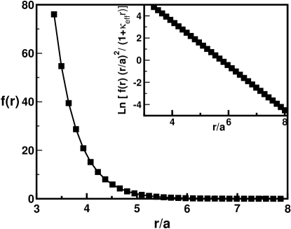
Figure 1:

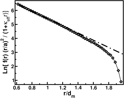
Figure 2:

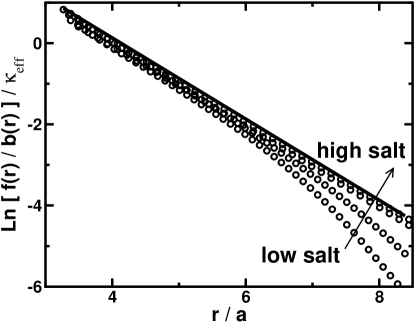
Figure 3:

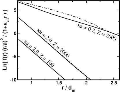
Figure 4:

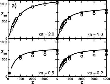
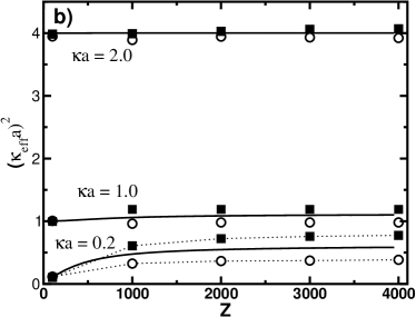
Figure 5:

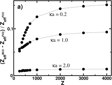
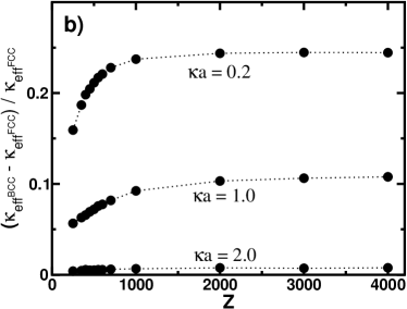
Figure 6:

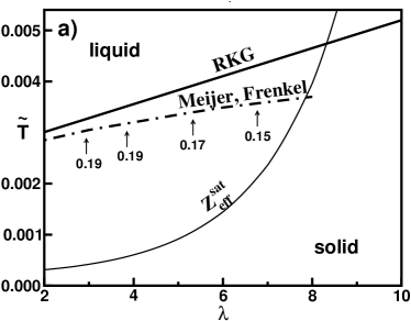
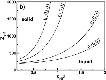
Figure 7:

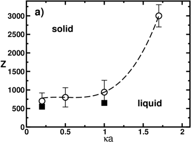
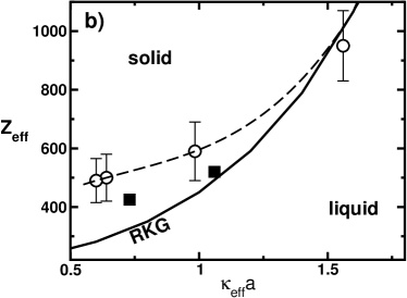
Figure 8:

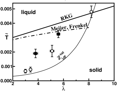
Figure 9:

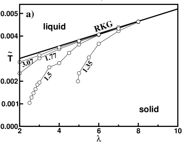
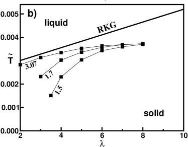
Figure 10:

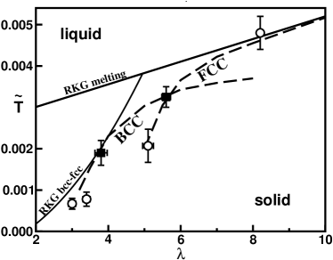
Figure 11:

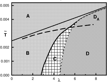
Figure 12:

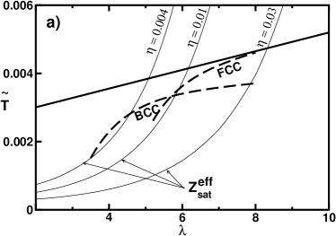
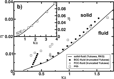
Figure 13:

References

- (1) E.J.W. Verwey and J.T.G. Overbeek, Theory of the Stability of Lyophobic Colloids (Elsevier, Amsterdam, 1948).
- (2) C.N. Likos, Phys. Rep.-Rev. Sec. Phys. Lett. 348, 267 (2001).
- (3) Y. Levin, Rep. Prog. Phys. 65, 1577 (2002).
- (4) P. Attard, Current opinion in colloidal interfaces science 6, 366 (2001).
- (5) H. Löwen and J.P. Hansen, Annu. Rev. Phys. Chem. 51, 209 (2000).
- (6) L. Belloni, J.Phys.: Condens. Matter 12, R549 (2000).
- (7) J.C. Crocker and D.G. Grier, Phys. Rev. Lett. 73, 352 (1994).
- (8) K. Vondermasse, J. Bongers, A. Mueller, and H. Versmold, Langmuir 10, 1351 (1994).
- (9) J.C. Crocker and D.G. Grier, Phys. Rev. Lett. 77, 1897 (1996).
- (10) P. Linse, J. Chem. Phys. 94, 8227 (1991).
- (11) H. Löwen and E. Allahyarov, J.Phys.: Condens. Matter 10, 4147 (1998).
- (12) J.Z. Wu, D. Bratko, H.W. Blanch, and J.M. Prausnitz, J. Chem. Phys. 113, 3360 (2000).
- (13) C. Russ, R. van Roij, M. Dijkstra, and H.H. von Grünberg, Phys. Rev. E 66, 011402 (2002).
- (14) R. Tehver, A. Ancilotto, F. Toigo, J. Koplik, and J.R. Banavar, Phys. Rev. E 59, R1335 (1999).
- (15) M. Fushiki, J. Chem. Phys. 97, 6700 (1992).
- (16) R.L. Henderson, Phys. Lett. A 49, 197 (1974).
- (17) P. Attard, Phys. Rev. A 45, 3659 (1992).
- (18) L. Reatto and M. Tau, J. Chem. Phys. 86, 6474 (1987).
- (19) J. Ram and Y. Singh, J. Chem. Phys. 66, 924 (1977).
- (20) R. Klein, H.H. von Grünberg, C. Bechinger, M. Brunner, and V. Lobaskin, J.Phys.: Condens. Matter 14, 7631 (2002).
- (21) M. Brunner, C. Bechinger, W. Strepp, V. Lobaskin, and H.H. von Grünberg, Europhys. Lett. 58, 926 (2002).
- (22) J.A. Barker and D. Henderson, Rev. Mod. Phys. 48, 587 (1976).
- (23) B.M. Axilrod and E. Teller, J. Chem. Phys. 11, 299 (1943).
- (24) M. Tau, L. Reatto, R. Magli, P.A. Egelstaff, and F. Barocchi, J.Phys.: Condens. Matter 1, 7131 (1989).
- (25) N. Jakse, J.M. Bomont, and J.L. Bretonnet, J. Chem. Phys. 116, 8504 (2002).
- (26) J.A. Barker, R.A. Fisher, and R.O. Watts, Mol. Phys. 21, 657 (1971).
- (27) R. Bukowski and K. Szalewicz, J. Chem. Phys. 114, 9518 (2001).
- (28) J.M. Bomont and J.L. Bretonnet, Phys. Rev. B 65, 224203 (2002).
- (29) P.B. Warren, J. Chem. Phys. 112, 4683 (2000).
- (30) B. Beresford-Smith, D.Y. Chan, and D.J. Mitchell, J. Colloid Interface Sci. 105, 216 (1984).
- (31) R. van Roij and R. Evans, J.Phys.: Condens. Matter 11, 14 (1999).
- (32) P. Linse, J. Chem. Phys. 113, 4359 (2000).
- (33) P. Linse and V. Lobaskin, Phys. Rev. Lett. 83, 4208 (1999).
- (34) P. Linse and V. Lobaskin, J. Chem. Phys. 112, 3917 (2000).
- (35) M. Dijkstra and R. van Roij, J.Phys.: Condens. Matter 10, 1219 (1998).
- (36) N.G. Almarza, E. Lomba, G. Ruiz, and C.F. Tejero, Phys. Rev. Lett. 86, 2038 (2001).
- (37) A.A. Louis, J.Phys.: Condens. Matter 14, 9187 (2002).
- (38) A.A. Louis, P. G. Bolhuis, J. P. Hansen, and E.J. Meijer, Phys. Rev. Lett. 85, 2522 (2000).
- (39) P. G. Bolhuis, A. A. Louis, and J.P. Hansen, Phys. Rev. E 64, 021801 (2001).
- (40) C.F. Tejero, J.Phys.: Condens. Matter 15, S395 (2002).
- (41) J. Dobnikar, D. Halozan, M. Brumen, H.H. von Grünberg, and R.Rzehak, Comput. Phys. Commun. (submitted) (2002).
- (42) G. Donnan, Chem. Rev. 1, 73 (1924).
- (43) J. Th. G. Overbeek, Prog. Biophys. and Biophys. Chem. 6, 57 (1956).
- (44) T.L. Hill, Disc. Faraday Soc. 21, 31 (1956).
- (45) V. Reus, L. Belloni, T. Zemb, N. Lutterbach, and H. Versmold, J. Phys. II France 7, 603 (1997).
- (46) M.N. Tamashiro, Y. Levin, and M.C. Barbosa, Eur. Phys. J. B 1, 337 (1998).
- (47) M. Deserno and H.H. von Grünberg, Phys. Rev. E 66, 011401 (2002).
- (48) D. Andelman, in Structure and Dynamics of Membranes, edited by R. Lipowsky and E. Sackmann (North Holland, Amsterdam, 1995), p. 603.
- (49) S. Levine, J. Chem. Phys. 7, 831 (1939).
- (50) S.L. Brenner and R. E. Roberts, J. Phys. Chem. 77, 2367 (1973).
- (51) We believe that the present article adresses the chemical physics community and that the results presented are new, relevant and suitable for publication in your journal. E.S. Reiner and C. J. Radke, J. Chem. Soc. Farad. Trans. 86, 3901 (1990).
- (52) E. Trizac and J.P. Hansen, Phys. Rev. E 56, 3137 (1997).
- (53) M. Deserno and C. Holm, in Proceedings of NATO Advanced Study Institute on Electrostatic Effects in Soft Matter and Biophysics, edited by C. Holm, P. Kekicheff, and R. Podgornik (Kluwer, Drodrecht, 2001), p. 27.
- (54) N.N. Tamashiro and H. Schiessel, cond-mat (preprint) 0210245, (2002).
- (55) R. Podgornik and B. Žekš, J. Chem. Soc. Faraday Trans. 84, 611 (1988).
- (56) R.D. Coalson and A. Duncan, J. Chem. Phys. 97, 5653 (1992).
- (57) I. Borukhov, D. Andelman, and H. Orland, Electrochimica Acta 46, 221 (2000).
- (58) R.R.Netz and H. Orland, Eur. Phys. J. E 1, 203 (2000).
- (59) H. Löwen, J.P. Hansen, and P.A. Madden, J. Chem. Phys. 98, 3275 (1993).
- (60) V. Lobaskin and P. Linse, J. Chem. Phys. 111, 4300 (1999).
- (61) V. Lobaskin, A.Lyubartsev, and P. Linse, Phys. Rev. E 63, 020401 (2001).
- (62) R.D. Groot, J. Chem. Phys. 95, 9191 (1991).
- (63) S.L. Carnie and G.M. Torrie, Adv. Chem. Phys. 56, 142 (1984).
- (64) M. D. Gilson, J. A. McCammon, and J. D. Madura, J. Comp. Chem. 16, 1081 (1995).
- (65) H. Müller, Kolloidchem. Beihefte 26, 257 (1928).
- (66) C. A. J. Fletcher, Computational Techniques for Fluid Dynamics I (Springer, Heidelberg, 1991).
- (67) J. Ortega and W. C. Rheinboldt, Iterative solution of nonlinear equations in several variables (Academic Press, New York, 1970).
- (68) P. E. Klöden and E. Platen, umerical Solution of Stochastic Differential Equations (Springer, Heidelberg, 1992).
- (69) H. C. Öttinger, Stochastic Processes in Polymeric Fluids (Springer, Heidelberg, 1996).
- (70) H. Löwen and G. Kramposthuber, Europhys. Lett. 23, 673 (1993).
- (71) S. Alexander, P.M. Chaikin, P. Grant, G.J. Morales, P. Pincus, and D. Hone, J. Chem. Phys. 80, 5776 (1984).
- (72) J. Yamanaka, H. Yoshida, T. Koga, N. Ise, and T. Hashimoto, Phys. Rev. Lett. 80, 5806 (1998).
- (73) Y. Monovouskas and A.P. Gast, J. Colloid Interface Sci. 128, 533 (1989).
- (74) L. Belloni, Colloids Surfaces A 140, 227 (1998).
- (75) P. Linse, J. Chem. Phys. 94, 3817 (1991).
- (76) M. Fushiki, J. Chem. Phys. 89, 7445 (1988).
- (77) L. Belloni, J. Chem. Phys. 85, 519 (1986).
- (78) M. Quesada-Perez, J. Callejas-Fernandez, and R. Hidalgo-Alvarez, Adv. Colloid Interface Sci. 95, 295 (2002).
- (79) L. Bocquet, E. Trizac, and M. Aubouy, J. Chem. Phys. 117, 8138 (2002).
- (80) E. Trizac, L. Bocquet, and M. Aubouy, Phys. Rev. Lett. 89, 248301 (2002).
- (81) M.O. Robbins, K. Kremer, and G.S. Grest, J. Chem. Phys. 88, 3286 (1988).
- (82) D. Frenkel and D.J. Meijer, J. Chem. Phys. 94, 2269 (1991).
- (83) H. Löwen, Phys. Rep.-Rev. Sec. Phys. Lett. 237, 76 (1994).
- (84) A.K. Arora and B.V.R. Tata, Adv. Colloid Interface Sci. 78, 49 (1998).
- (85) J. Chakrabarti, H.R. Krishnamurthy, S. Sengupta, and A.K. Sood, in Ordering and Phase Transition in Charged Colloids, edited by A.K. Arora and B.V.R. Tata (VCH Publishers, New York, 1995), p. 235.
- (86) P.S. Kuhn, A. Diehl, Y. Levin, and M.C. Barbosa, Physica A 247, 235 (1997).
- (87) D.C. Wang and A.P. Gast, J.Phys.: Condens. Matter 11, 10133 (1999).
- (88) C.F. Tejero, in Chemical Applications of Density-Functional Theory, ACS Symp. Ser. (ACS, New York, 1996), p. 297.
- (89) D.B. Lukatsky and S.A. Safran, Phys. Rev. E 63, 011405 (2001).
- (90) D.C. Wang and A.P. Gast, J. Chem. Phys. 112, 2826 (2000).
- (91) R.O. Rosenberg and D. Thirumalai, Phys. Rev. A 36, 5690 (1987).
- (92) G. Dupont, S. Moulinasse, J.P. Ryckaert, and M. Baus, Mol. Phys. 79, 453 (1993).
- (93) E.J. Meijer and F. El Azhar, J. Chem. Phys. 106, 4678 (1997).
- (94) F. El Azhar, M. Baus, J.P. Ryckaert, and E.J. Meijer, J. Chem. Phys. 112, 5121 (2000).
- (95) F.A. Lindemann, Z. Phys. 11, 609 (1910).
- (96) H. Oshima, T. Healy, and L.R. White, J. Colloid Interface Sci. 90, 17 (1982).
- (97) A. Phillipse, private communication.
- (98) A. Yethiraj and A. van Blaaderen, Nature, in press, (2002).