Event-plane flow analysis without non-flow effects

Abstract

The event-plane method, which is widely used to analyze anisotropic flow in nucleus-nucleus collisions, is known to be biased by nonflow effects, especially at high $p_{t}$. Various methods (cumulants, Lee-Yang zeroes) have been proposed to eliminate nonflow effects, but their implementation is tedious, which has limited their application so far. In this paper, we show that the Lee-Yang-zeroes method can be recast in a form similar to the standard event-plane analysis. Nonflow correlations are strongly suppressed by using the information from the length of the flow vector, in addition to the event-plane angle. This opens the way to improved analyses of elliptic flow and azimuthally-sensitive observables at RHIC and LHC.

I Introduction

Studies of particle production at the BNL Relativistic Heavy Ion Collider (RHIC) have revealed strong collective effects: in particular, the azimuthal distribution transverse to the direction of the colliding nuclei has sizable anisotropies, a phenomenon called anisotropic flow. The main component of this anisotropy, elliptic flow, has been extensively measured for several beam energies and collision systems Ackermann:2000tr ; Back:2002gz ; Adler:2003kt .

Anisotropic flow is most often analyzed using the event-plane method Poskanzer:1998yz . This analysis technique is plagued by systematic errors due to nonflow effects Ollitrault:1995dy . There are other sources of systematic errors, such as fluctuations Miller:2003kd ; Alver:2006wh , but nonflow effects are expected to be the dominant source of error at high $p_{t}$ Adams:2004bi , where they are likely to originate from jet-like (hard) correlations; they are expected to be even larger at the LHC. The purpose of this paper is to show that nonflow effects can be suppressed at the expense of a slight modification of the event-plane method.

Anisotropic flow of selected produced particles, in a given part of phase-space, is defined as their azimuthal correlation with the reaction plane Voloshin:1994mz

$$v_{n}\equiv\left\langle\cos(n(\phi-\Phi_{RP}))\right\rangle$$ (1)

where $n$ is an integer ($v_{1}$ is directed flow, $v_{2}$ is elliptic flow), $\phi$, $\Phi_{RP}$ and angular brackets denote respectively the azimuth of the particle under study, the azimuth of the reaction plane, and an average over particles and events. Since $\Phi_{RP}$ is not known experimentally, $v_{n}$ cannot be measured directly.

The most commonly used method to estimate $v_{n}$ is the event-plane method Poskanzer:1998yz . In each event, one constructs an estimate of the reaction plane $\Phi_{RP}$, the “event plane” $\Phi_{EP}$ Danielewicz:1985hn . The anisotropic flow coefficients are then estimated as

$$v_{n}{\{\rm EP}\}\equiv\frac{1}{R}\left\langle\cos(n(\phi-\Phi_{EP}))\right\rangle,$$ (2)

where $R=\left\langle\cos(n(\Phi_{EP}-\Phi_{RP}))\right\rangle$ is the event-plane resolution, which corrects for the difference between $\Phi_{EP}$ and $\Phi_{RP}$. This resolution is determined in each class of events through a standard procedure Ollitrault:1997di .

The analogy between Eq. (2) and Eq. (1) makes the method rather intuitive, but its practical implementation has a few subtleties:

• One must remove autocorrelations: the particle under study should not be used in defining the event plane, otherwise there is a trivial correlation between $\phi$ and $\Phi_{EP}$ Danielewicz:1985hn . This means in practice that one must keep track of which particles have been used in defining the event plane, so as to remove them if necessary.

• More generally, there are sources of correlation, other than flow, through which the particle under study can be correlated with a particle used in defining the event plane. Such correlations, called “nonflow effects”, result in $v_{n}\{{\rm EP}\}\not=v_{n}$ and must be suppressed. This cannot be done in a systematic way, but rapidity gaps are believed to reduce nonflow effects Adler:2003kt ; Voloshin:2006wi .

• Event-plane flattening procedures must be implemented to correct for azimuthal asymmetries of the detector acceptance Poskanzer:1998yz .

A systematic way of suppressing nonflow effects is to use improved methods such as cumulants Borghini:2001vi or Lee-Yang zeroes Bhalerao:2003xf . Cumulants have been used at SPS Alt:2003ab and RHIC Adler:2002pu ; Adams:2004bi . Lee-Yang zeroes have been implemented at SIS Bastid:2005ct and at RHIC Abelev:2008ed . They are comparatively much less used than the event-plane method, and one reason is that the event-plane method is deemed more intuitive and handy.

In this paper, we show that the method of flow analysis based on Lee-Yang zeroes can be rewritten in a way which is mathematically equivalent to the original formulation Bhalerao:2003xf , but formally analogous to the event-plane method, which makes it more intuitive. The corresponding estimate of $v_{n}$ is defined as

$$v_{n}\{{\rm LYZ}\}\equiv\left\langle W_{R}\cos(n(\phi-\Phi_{EP}))\right\rangle,$$ (3)

where $\Phi_{EP}$ is the same as in Eq. (2), and $W_{R}$ is an event weight as defined in this paper. The formal analogy with the event-plane method, Eq. (2), is obvious. The advantage of the improved event-plane method defined by Eq. (3) over the standard event-plane method is that both autocorrelations and nonflow effects are automatically suppressed.

The paper is organized as follows. In Sec. II, we describe the method for a detector with perfect azimuthal symmetry, and we explain why it automatically removes autocorrelations and nonflow correlations, in contrast to the standard event-plane method. Readers interested in applying the method should read Appendix A, which describes the recommended practical implementation, taking into account anisotropies in the detector acceptance. In Sec. III, we present results of Monte-Carlo simulations, where results obtained with the Lee-Yang zeroes method are compared to those obtained with 2- and 4-particle cumulants. Sec. IV concludes with a discussion of where the method should be applicable, and of its limitations.

II Description of the method

II.1 The flow vector

The first step of the flow analysis is to evaluate, for each event, the flow vector of the event. It is a two-dimensional vector ${\bf Q}=(Q_{x},Q_{y})$ defined as

$$Q_{x}=Q\cos(n\Phi_{EP}) \equiv \sum_{j=1}^{M}w_{j}\,\cos(n\phi_{j})$$ (4)

$$Q_{y}=Q\sin(n\Phi_{EP}) \equiv \sum_{j=1}^{M}w_{j}\,\sin(n\phi_{j}),$$ (5)

where the sum runs over all detected particles footnote1 . $M$ is the observed multiplicity of the event, $\phi_{j}$ are the azimuthal angles of the particles measured with respect to a fixed direction in the laboratory. The coefficients $w_{j}$ in Eq. (4) are weights depending on transverse momentum, particle mass and rapidity. The best weight, which minimizes the statistical error (or, equivalently, maximizes the resolution) is $v_{n}$ itself, $w_{j}(p_{T},y)\propto v_{n}(p_{T},y)$ Borghini:2000sa . A reasonable choice for elliptic flow measurements at RHIC (and probably LHC) is $w=p_{T}$.

If collective flow is present, the azimuthal angles $\phi_{j}$ and the event plane $\Phi_{EP}$ are correlated with the true reaction plane $\Phi_{RP}$, and the goal of the flow analysis is to measure this correlation. This is usually done within a set of events belonging to the same centrality class. Integrated flow is defined as the average value of the projection of ${\bf Q}$ onto the true reaction plane:

$$V_{n}\equiv\left\langle Q\cos(n(\Phi_{EP}-\Phi_{RP}))\right\rangle$$ (6)

where angular brackets denote an average over events in the same centrality class. We use a capital letter for $V_{n}$ because it is in general a dimensionful quantity: it is the weighted sum of the $v_{n}$’s of individual particles, according to Eqs. (1) and (4). The flow vector fluctuates around this average value because the multiplicity is finite. These fluctuations can be modeled using the central limit theorem. The resulting distribution of $Q$ is Ollitrault:1995dy :

$$\frac{dN}{dQ}=\frac{2\chi^{2}Q}{V_{n}^{2}}\exp\left(-\chi^{2}\left(\frac{Q^{2}}{V_{n}^{2}}+1\right)\right)I_{0}\left(\frac{2\chi^{2}Q}{V_{n}}\right),$$ (7)

where $\chi$ is a dimensionless quantity called the resolution parameter, which characterizes the relative magnitude of collective flow and statistical fluctuations. The resolution $R$ in Eq. (2) increases from $0$ to $1$ as $\chi$ goes from $0$ to $+\infty$. Fig. 1 illustrates the distribution of $Q$ for two values of $\chi$. For $\chi\gg 1$, this distribution is a narrow peak centered at $Q=V_{n}$.

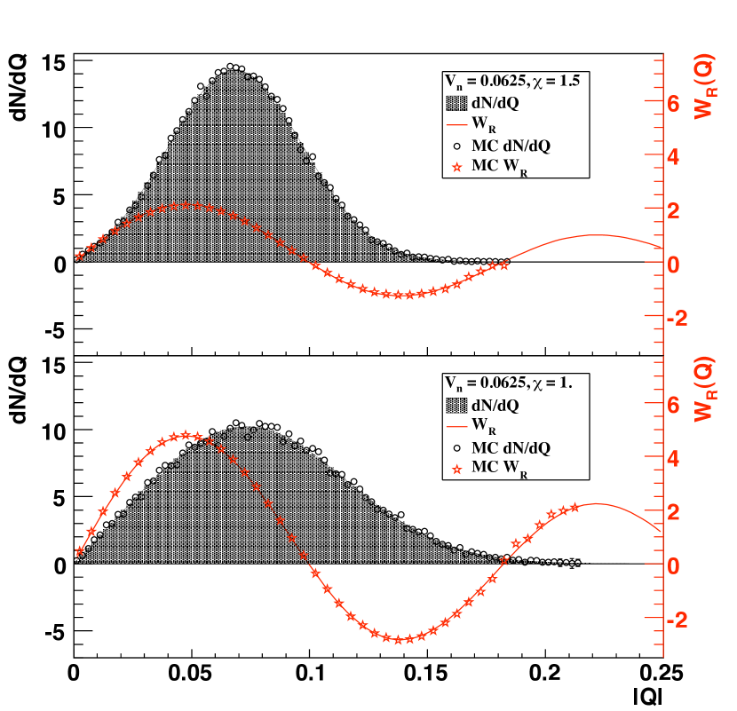
Figure 1: (Color online) Shaded area: probability distribution of $Q$, Eq. (7), with $V_{n}=0.0625$. Top: $\chi=1.5$, corresponding to a resolution $R=0.86$ in the standard analysis (see Eq. (2)). Bottom: $\chi=1$, corresponding to a resolution $R=0.71$. This is the typical value for a semi-central Au-Au collision at RHIC analyzed by the STAR TPC Adams:2004bi . Solid curve: weight $W_{R}$ defined by Eqs. (16) and (17). Open circles: histograms of the distribution of $Q$ obtained in the Monte-Carlo simulation of Sec. III, following the procedure detailed in Appendix A. Stars: weights obtained in Sec. III.

Lee-Yang zeroes use the projection of the flow vector onto a fixed, arbitrary direction making an angle $n\theta$ with respect to the $x$-axis. We denote this projection by $Q_{\theta}$:

$$Q_{\theta}\equiv Q_{x}\cos n\theta+Q_{y}\sin n\theta=Q\cos(n(\Phi_{EP}-\theta)).$$ (8)

II.2 Integrated flow

We now explain how the integrated flow $V_{n}$, defined by Eq. (6), is obtained. We define the complex-valued function:

$$G_{\theta}(r)\equiv\left\langle e^{irQ_{\theta}}\right\rangle\equiv\frac{1}{N_{\rm evts}}\sum_{\rm events}e^{irQ_{\theta}}.$$ (9)

If there is no collective flow, the probability distribution of $Q_{\theta}$ is a Gaussian due to the central limit theorem (if $M\gg 1$). Its Fourier transform $G_{\theta}(r)$ is also a Gaussian. Collective flow results in oscillations of $G_{\theta}(r)$ around zero: In the ideal case where the multiplicity is so large that fluctuations can be neglected, $\Phi_{EP}\simeq\Phi_{RP}$ and $Q\simeq V_{n}$. Inserting Eq. (8) into (9) and averaging over $\Phi_{RP}$, one obtains

$$G_{\theta}(r)\simeq J_{0}(rV_{n}),$$ (10)

where $J_{0}(x)$ denotes the Bessel function of the first kind of order 0, which oscillates around 0. Finite multiplicity fluctuations result in a gaussian smearing of $G_{\theta}(r)$, but quite remarkably, the location of the zeroes is unchanged, up to statistical fluctuations due to the finite number of events Bhalerao:2003yq .

As a consequence, the modulus $|G_{\theta}(r)|$ has sharp minima for positive $r$, which can be estimated numerically. The position of the first minimum, $r_{\theta}$, is used to estimate $V_{n}$, using Eq. (10):

$$V_{n}=\frac{j_{01}}{r_{\theta}},$$ (11)

where $j_{01}\simeq 2.40483$ is the first zero of $J_{0}(x)$. One may also check, as a consistency test, that $|G_{\theta}(r_{\theta})|=0$ within statistical errors Bhalerao:2003yq .

The above procedure only makes use of the projection of the flow vector onto an arbitrary direction $\theta$. For a perfect detector, azimuthal symmetry ensures that $r_{\theta}$ is independent of $\theta$, up to statistical errors. In practice, however, it is recommended to repeat the analysis for several values of $\theta$ (see Appendix A).

II.3 Differential flow and event weight

We now derive the expression of the event weight in Eq. (3), which is the crucial improvement of our paper over the standard event-plane method. The goal is to measure the differential flow $v_{n}$ of selected produced particles. $v_{n}$ can be obtained by shifting the weights $w_{j}$ of the selected particles in Eq. (4) by an infinitesimal quantity $\varepsilon$, $w^{\prime}_{j}=w_{j}+\varepsilon$, and computing the integrated flow $V^{\prime}_{n}$ with the new weights. The differential flow is then simply given by $v_{n}=\delta V_{n}/\varepsilon$, with $\delta V_{n}=V^{\prime}_{n}-V_{n}$. Differentiating Eq. (11),

$$v_{n}\{\rm LYZ\}=\frac{\delta V_{n}}{\varepsilon}=-\frac{V_{n}}{\varepsilon}\frac{\delta r_{\theta}}{r_{\theta}},$$ (12)

where $\delta r_{\theta}$ denotes the shift of the zero. Differentiating the condition $\langle e^{ir_{\theta}Q_{\theta}}\rangle=0$, one obtains

$$\delta r_{\theta}\left\langle Q_{\theta}e^{ir_{\theta}Q_{\theta}}\right\rangle+r_{\theta}\left\langle\delta Q_{\theta}e^{ir_{\theta}Q_{\theta}}\right\rangle=0.$$ (13)

For an event containing one selected particle, Eqs. (4) and (8) give $\delta Q_{\theta}=\varepsilon\cos(n(\phi-\theta))$, where $\phi$ is the azimuth of the selected particle. Eq. (12) then gives

$$v_{n}\{\rm LYZ\}=V_{n}\frac{\left\langle\cos(n(\phi-\theta))e^{ir_{\theta}Q_{\theta}}\right\rangle}{\left\langle Q_{\theta}e^{ir_{\theta}Q_{\theta}}\right\rangle},$$ (14)

where the average in the numerator is over selected particles, and the average in the denominator is over events. In this expression, $\theta$ is an arbitrary reference angle. Both the numerator and the denominator are expected to be independent of $\theta$, up to asymmetries in the detector acceptance, and statistical fluctuations. In practice, we recommend to first take the ratio and then average over $\theta$, as explained in Sec.A.2. Here, we derive simple approximate expressions by assuming that $r_{\theta}$ is independent of $\theta$, and by averaging the numerator and the denominator over $\theta$ before taking the ratio. We thus obtain:

$$v_{n}\{\rm LYZ\}=V_{n}\frac{\left\langle\cos(n(\phi-\Phi_{EP}))J_{1}(r_{\theta}Q)\right\rangle}{\left\langle QJ_{1}(r_{\theta}Q)\right\rangle},$$ (15)

where $J_{1}(x)$ is the derivative of $-J_{0}(x)$. Identifying Eq. (15) with Eq. (3), we obtain the event weight

$$W_{R}\equiv\frac{1}{C}J_{1}(r_{\theta}Q),$$ (16)

where $C$ is a normalization constant which can be computed using the distribution (7):

$$C=\frac{1}{V_{n}}\left\langle QJ_{1}(r_{\theta}Q)\right\rangle=\exp\left(-\frac{j_{01}^{2}}{4\chi^{2}}\right)J_{1}(j_{01}).$$ (17)

The difference with the standard event-plane analysis is that each event is given a weight (16) which depends on the length of the flow vector $Q$, a quantity which is not used in the standard analysis. Eq. (16) involves the integrated flow $V_{n}$ through $r_{\theta}$, which must be determined in a first pass through the data.

Fig. 1 displays the variation of $W_{R}$ with $Q$, for two values of the resolution parameter. For $\chi\gg 1$, the distribution of $Q$ is a narrow peak centered at $Q=V_{n}$. Therefore, the weight defined by Eqs. (16) and (17) is close to $1$ for all events. If $\chi$ is smaller, the distribution of $Q$ is wider, and $W_{R}$ is negative for some events. These negative weights are required in order to subtract nonflow effects. On the other hand, they also subtract part of the flow. In order to compensate for this effect, the global normalization of the weight increases when $\chi$ decreases (as illustrated in Fig. 1 by the fact that the amplitude of the curve showing the weight changes for different values of $\chi$). This qualitatively explains the $\chi$ dependence in Eq. (17).

The weight (16) vanishes linearly at $Q=0$. This is physically intuitive. Given that the flow vector is obtained by summing over all particles, one increases the relative weight of collective flow over individual, random motion of the particles. If the flow vector is small in an event, it means that the random motion hides the collective motion in this particular event, which is therefore of little use for the flow analysis.

II.4 Nonflow effects and autocorrelations

We now explain why the method suppresses nonflow effects and autocorrelations on the basis of two simple examples.

As a first example, we assume that each particle splits into two particles with identical momenta, roughly imitating the effect of resonance decays or track splitting in a detector. This splitting does not change the anisotropic flow $v_{n}$, defined by Eq. (1), but it introduces nonflow correlations, which bias standard analyses as will be shown in Sec. III. The splitting leaves $v_{n}\{\rm LYZ\}$ unchanged: it multiples both the flow vector, Eq. (4) and the integrated flow $V_{n}$, Eq. (6) by 2. Therefore $r_{\theta}$ in Eq. (11) is divided by 2, and $v_{n}\{\rm LYZ\}$ defined by Eq. (14) is unchanged.

As a second example, we consider the situation where there is collective flow in the system, but the selected particles have $v_{n}=0$. We further assume that the selected particles are uncorrelated with the other particles. In the standard event-plane method, one needs to subtract the selected particles from the flow vector (4), otherwise autocorrelations yield $v_{n}\{EP\}>0$. We now show that $v_{n}\{LYZ\}=0$, even if selected particles are included in the flow vector.

We separate the flow vector, Eq. (4), into the contribution of selected particles, ${\bf Q}_{\rm sel.}$, and other particles ${\bf Q}_{\rm others}$.

$${\bf Q}={\bf Q}_{\rm sel.}+{\bf Q}_{\rm others}.$$ (18)

Our estimate of $v_{n}$ is defined by Eq.(14). Since the flow vector appears in an exponential, the contributions of selected particles and other particles can be written as a product of two independent factors:

$$v_{n}=V_{n}\frac{\left\langle\cos(n(\phi-\theta))e^{ir_{\theta}(Q_{\rm sel.})_{\theta}}\right\rangle\left\langle e^{ir_{\theta}(Q_{\rm others})_{\theta}}\right\rangle}{\left\langle Q_{\theta}e^{ir_{\theta}Q_{\theta}}\right\rangle},$$ (19)

Let us define $G_{\rm others,\theta}(r)$ by replacing $Q_{\theta}$ with $Q_{\rm others,\theta}$ in Eq. (9). Following the same reasoning as in Sec. II.2, the first zero of $G_{\rm others,\theta}$ depends on the integrated flow $V_{n,{\rm others}}$ of other particles. We have assumed that $v_{n}=0$ for selected particles, therefore $V_{n,{\rm others}}=V_{n}$, and

$$\left\langle e^{ir_{\theta}(Q_{\rm others})_{\theta}}\right\rangle=\left\langle e^{ir_{\theta}Q_{\theta}}\right\rangle=0.$$ (20)

Inserting into Eq. (19), we find

$$v_{n}\{{\rm LYZ}\}=0,$$ (21)

up to statistical fluctuations. This proof can easily be generalized to the situation where each selected particle is correlated with a few additional particles (e.g. within a jet) which are not correlated with the bulk of particles producing collective flow.

We have constructed two simple examples where Lee-Yang zeroes are able to eliminate nonflow effects and autocorrelations. In actual experiments, however, flow and nonflow effects are likely to be mingled, and detailed simulations must be carried out to determine to what extent the suppression is effective.

III Simulations

To check the validity of the procedure described in this paper and to compare it with other analysis methods $N=$ 28 000 events were simulated with a Monte-Carlo program dubbed GeVSim gevsim . In GeVSim the $v_{2}$ and the particle yield as function of transverse momentum and pseudorapidity are generated according to a user-defined parameterization. For these simulations events were generated using a linear dependence of $v_{2}(p_{t})$ in the range 0–2 GeV/$c$, above 2 GeV/$c$ the $v_{2}(p_{t})$ was set constant. The average elliptic flow is $\langle v_{2}\rangle=0.0625$. We then reconstructed $v_{2}(p_{t})$ from the simulated events using several methods: the Lee-Yang-zeroes method described in Appendix A, as well as 2- and 4-particle cumulants Borghini:2001vi . The corresponding estimates of $v_{2}$ are denoted by $v_{2}\{{\rm LYZ}\}$, $v_{2}\{2\}$ and $v_{2}\{4\}$, respectively. $v_{2}\{2\}$ is generally close to $v_{2}$ from the traditional event-plane method; both are biased by nonflow effects. On the other hand, $v_{2}\{4\}$ is expected to be close to $v_{2}\{{\rm LYZ}\}$, with the bias from nonflow effects suppressed. The weight $w_{j}$ in Eq. (4) was chosen identically $1/M$ for all particles, with $M$ the event multiplicity, so that the integrated flow $V_{n}$ defined by Eq. (1) coincides with the average elliptic flow, i.e., $V_{n}=0.0625$. The analysis was repeated twice by varying the multiplicity $M$ used in the flow analysis: the values 256 and 576 were used, so as to achieve a resolution of $\chi=$1 and 1.5. footnote2 .

Fig. 2 shows the generated (input) $v_{2}(p_{t})$ together with the reconstructed $v_{2}(p_{t})$ using cumulants and Lee-Yang zeroes for $\chi=1$. The upper panel shows the results in the case where all correlations are due to flow. In this case, all three methods yield the correct $v_{2}(p_{t})$ and $\langle v_{2}\rangle$ within statistical uncertainties (see Table 1), which are twice larger for $v_{2}\{4\}$ and $v_{2}\{{\rm LYZ}\}$ than for $v_{2}\{2\}$ (see Sec. A.3).

In the lower panel, simulations are shown which include nonflow effects. Because GeVSim generates no nonflow, nonflow correlations are introduced by using each input track twice, as in Sec. II.4. Experiments at RHIC have shown Adams:2004bi that nonflow effects are larger at high-$p_{t}$ (probably due to jet-like correlations), and a realistic simulation of nonflow effects should take into account this $p_{t}$ dependence. Our simplified implementation, which does not, is not realistic. It is merely an illustration of the impact of nonflow effects on the flow analysis. Fig. 2 shows that due to nonflow effects, the method based on two-particle cumulants ($v_{2}\{2\}$) overestimates the average elliptic flow $\langle v_{2}\rangle$. The error on the average elliptic flow is larger than 20% (see Table 1, right column). The transverse-momentum dependence of $v_{2}(p_{t})$ is also not correct, with an excess at low $p_{t}$ by $0.03$. By contrast, the results from 4-particle cumulants ($v_{2}\{4\}$) and Lee-Yang zeroes ($v_{2}\{{\rm LYZ}\}$) are, within statistical uncertainties, in agreement with the true generated flow distribution. This shows that the method presented in this paper is able to remove nonflow effects.

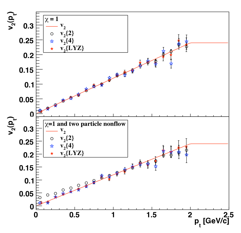
Figure 2: (Color online) Differential elliptic flow $v_{2}(p_{t})$ reconstructed using different methods; in the upper panel from events where no nonflow was included, in the lower panel from events with nonflow. The line in both panels is the input $v_{2}$.

Table 1: Value of the average elliptic flow $\langle v_{2}\rangle$ reconstructed, using different methods, from simulated data with and without nonflow effects. The input value is $\langle v_{2}\rangle=0.0625$.

Method	Flow only	Flow+nonflow
$v_{2}\{2\}$	$0.0626\pm 0.0003$	$0.0764\pm 0.0004$
$v_{2}\{4\}$	$0.0624\pm 0.0005$	$0.0627\pm 0.0007$
$v_{2}\{{\rm LYZ}\}$	$0.0626\pm 0.0005$	$0.0629\pm 0.0007$

IV Discussion

Two effects limit the accuracy of flow analyses at high energy: nonflow effects and eccentricity fluctuations Miller:2003kd ; Alver:2006wh . The method presented in this paper is an improved event-plane method, which strongly suppresses the first source of uncertainty, nonflow effects. It has been argued Voloshin:2007pc that cumulants (and therefore Lee-Yang zeroes, which corresponds to the limit of large-order cumulants) also eliminate eccentricity fluctuations Miller:2003kd ; Alver:2006wh . However, a detailed study Alver:2008zza shows that even with cumulants, there may remain large effects of fluctuations in central collisions and/or small systems. This issue deserves more detailed investigation.

Letting aside the question of fluctuations, we now discuss which method of flow analysis should be used, depending on the situation. There are three main classes of methods: the standard event-plane method Poskanzer:1998yz , four-particle cumulants Borghini:2001vi , and the Lee-Yang-zeroes method presented in this paper. When the standard event-plane method is used, nonflow effects and eccentricity fluctuations are generally the main sources of uncertainty on $v_{n}$, and they dominate over statistical errors. The magnitude of this uncertainty is at least 10% at RHIC in semi-central collisions; it is larger for more central or more peripheral collisions, and also larger at high $p_{t}$. Unless statistical errors are of comparable magnitude as errors from nonflow effects, cumulants or Lee-Yang zeroes should be preferred over the standard method.

The main advantage of Lee-Yang zeroes, compared to cumulants, is that the method involves an event-plane angle. This is useful in particular for studying azimuthally dependent correlations Adams:2004wz ; Bielcikova:2003ku . Such studies cannot be done with cumulants, but they are straightforward with Lee-Yang zeroes. The only complication is that the azimuthal distribution of particle pairs generally involves sine terms Borghini:2004ra , in addition to the cosine terms of Eq. (1). These terms are simply obtained by replacing cos with sin in Eq. (3).

When studying anisotropic flow of individual particles, both cumulants and Lee-Yang zeroes can be applied. The cumulant method has been recently improved by directly calculating the cumulants Bilandzic:2010jr . With these improvements, both methods are expected to be essentially equivalent. The slight advantages of Lee-Yang zeroes are: 1) They are easier to implement. 2) They further reduce the error from nonflow effects. 3) The statistical error is slightly smaller if the resolution parameter $\chi>1$. For $\chi=0.8$, the error is only 35% larger with Lee-Yang zeroes than with 4-particle cumulants (and 4 times larger than with the event-plane method).

Our recommendation is that Lee-Yang zeroes should be used as soon as $\chi>0.8$. For small values of $\chi$, typically $\chi<0.6$, statistical errors on Lee-Yang zeroes blow up exponentially, which rules out the method; the statistical error on 4-particle cumulants also increases but more mildly, and their validity extends down to lower values of the resolution if very large event statistics is available.

A limitation of the present method is that it does not apply to mixed harmonics: this means that it cannot be used to measure $v_{1}$ and $v_{4}$ at RHIC and LHC using the event plane from elliptic flow Adams:2003zg . Note that $v_{1}$ can in principle be measured using Lee-Yang zeroes Borghini:2004ad using the “product” generating function, but this method cannot be recast in the form of an improved event-plane method. Higher harmonics such as $v_{4}$ also have a sensitivity to autocorrelations and nonflow effects, which is significantly reduced by using the product generating function Borghini:2001vi .

In conclusion, we have presented an improved event-plane method for the flow analysis, which automatically corrects for autocorrelations and nonflow effects. As in the standard method, each event has its event plane $\Phi_{EP}$, an estimate of the reaction plane, which is the same as for the standard method, except for technical details in the practical implementation. The trick which removes autocorrelations and nonflow effects is that there is in addition an event weight. Anisotropic flow $v_{n}$ is then estimated as a weighted average of $\cos(n(\phi-\Phi_{EP}))$. A straightforward application of this method would be to measure jet production with respect to the reaction plane at LHC. With the traditional event-plane method, such a measurement would require to subtract particles belonging to the jet from the event plane; in addition, strong nonflow correlations are expected within a jet, which would bias the analysis.

Appendix A Practical implementation

Before we describe the implementation of the method, let us mention that there are in fact two Lee-Yang-zeroes methods, depending on how the generating function is defined: the “sum generating function” makes explicit use of the flow vector Bhalerao:2003yq , while the “product generating function” Borghini:2004ke is constructed using the azimuthal angles of individual particles, and cannot be expressed simply in terms of the flow vector. Cumulants also exist in both versions, the “sum” Borghini:2000sa and the “product” Borghini:2001vi . For Lee-Yang zeroes, both the sum and the product give essentially the same result for the lowest harmonic Bastid:2005ct : the difference between results from the two methods is significantly smaller than the statistical error. On the other hand, the product generating function is significantly better than the sum generating function if one analyzes $v_{4}$ or $v_{1}$ Borghini:2004ad using mixed harmonics. The method described below is strictly equivalent to the sum generating function, although expressed in different terms. On the other hand, the product generating function cannot be recast in a form similar to the event-plane method, and will not be used here.

The method a priori requires two passes through the data, which are described in Sec. A.1 and Sec. A.2.

A.1 First pass: locating the zeroes

As with other flow analyses, one must first select events in some centrality class. The whole procedure described below must be carried out independently for each centrality class.

The flow vector $(Q_{x},Q_{y})$ is defined by Eq. (4). In contrast to the standard event-plane method, no flattening procedure is required to make the distribution of ${\bf Q}$ isotropic. Corrections for azimuthal anisotropies in the acceptance, which do not vary significantly in the event sample used, are handled using the procedure described below. We do not define the event plane $\Phi_{EP}$ as the azimuthal angle of the flow vector, as in Eq. (4). The procedure below defines both the event weight and the event plane.

The analysis uses the projection of the flow vector onto an arbitrary direction, see Eq. (8). In practice, the first pass should be repeated for several equally-spaced values of $n\theta$ between $0$ and $\pi$. This reduces the statistical error as shown by Eq. (29). For more than 5 values of $\theta$ the reduction is not significant anymore, so this number is recommended. For elliptic flow, for instance, $\theta$ takes the values $\theta=0,\pi/10,2\pi/10,3\pi/10,4\pi/10$.

One first computes the modulus $|G_{\theta}(r)|$, with $G_{\theta}$ defined by Eq. (9), as a function of $r$ for positive $r$. One determines numerically the first minimum of this function. This is the Lee-Yang zero. We denote its value by $r_{\theta}$. It must be stored for each $\theta$.

A.2 Second pass: determining the event weight, $w_{R}$, and the event plane, $\Phi_{EP}$.

In the second pass, one computes and stores, for each $\theta$, the following complex number:

$$D_{\theta}\equiv\frac{1}{j_{01}N_{\rm evts}}\sum_{\rm events}r_{\theta}Q_{\theta}e^{ir_{\theta}Q_{\theta}},$$ (22)

where $j_{01}\simeq 2.40483$. Except for statistical fluctuations and asymmetries in the detector acceptance, $D_{\theta}$ should be purely imaginary.

For each event, the event weight and the event plane are defined by

$$W_{R}\cos n\Phi_{EP} \equiv \left\langle{\rm Re}\left(\frac{e^{ir_{\theta}Q_{\theta}}}{D_{\theta}}\right)\cos n\theta\right\rangle_{\theta}$$ (23)

$$W_{R}\sin n\Phi_{EP} \equiv \left\langle{\rm Re}\left(\frac{e^{ir_{\theta}Q_{\theta}}}{D_{\theta}}\right)\sin n\theta\right\rangle_{\theta},$$ (24)

where Re denotes the real part, and angular brackets denote averages over the values of $\theta$ defined in subsection A.1. Our estimate of $v_{n}$, denoted by $v_{n}\{{\rm LYZ}\}$, is then defined by Eq. (3).

We now discuss how the angle $\Phi_{EP}$ defined by Eq. (23) compares with the event-plane from the standard analysis. First, we note that Eqs. (23) uniquely determine the angle $n\Phi_{EP}$ (modulo $2\pi$) only if the sign of $W_{R}$ is known. The simplest convention is $W_{R}>0$. In the simplified implementation described in Sec. II, however, where $\Phi_{EP}$ coincides with the standard event plane, $W_{R}$ defined by Eq. (16) can be negative, because the Bessel function changes sign (see Fig. 1). The convention $W_{R}>0$ then leads to a value of $n\Phi_{EP}$ which differs from the standard event plane by $\pi$, since changing the sign of $W_{R}$ amounts to shifting $n\Phi_{EP}$ by $\pi$ in Eqs. (23). This is illustrated in Fig. 3, which shows the distribution of the relative angle between $\Phi_{EP}$ and the standard event plane in the simulation of $v_{2}$ at LHC described in Sec. III. The distribution has two sharp peaks at 0 and $\pi/2$. The sign ambiguity produces the peak at $\pi/2$. The width of the peaks results from statistical fluctuations. The final result $v_{n}\{{\rm LYZ}\}$, given by Eq. (3), does not depend on the sign chosen for $W_{R}$.

If one wishes to have an event-plane as close as possible to the standard event plane, one may choose the following convention. Denoting by $\Phi_{EP}^{\rm std}$ the standard event plane, one computes the following quantity:

$$S\equiv W_{R}\cos n\Phi_{EP}\cos n\Phi_{EP}^{\rm std}+W_{R}\sin n\Phi_{EP}\sin n\Phi_{EP}^{\rm std},$$ (25)

where $W_{R}\cos n\Phi_{EP}$ and $W_{R}\sin n\Phi_{EP}$ are defined by Eq. (23). The sign of $W_{R}$ is then chosen as the sign of $S$, which ensures that $n\Phi_{EP}-n\Phi_{EP}^{\rm std}$ lies between $-\pi/2$ and $\pi/2$.

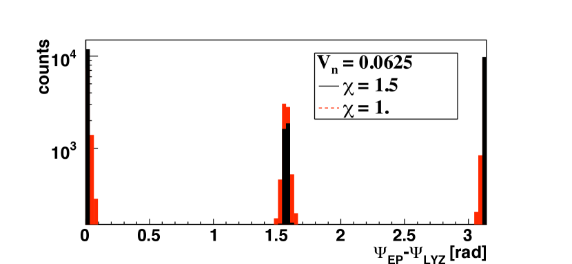
Figure 3: (Color online) Distribution of the relative angle between the event plane $\Phi_{EP}$ defined by Eq. (23), with $W_{R}>0$, and the standard event plane, for the reconstruction shown in Fig. 2.

The procedure described in this Appendix differs from the procedure described in Sec. II only in the case of non-uniform acceptance. This agreement can be seen in Fig. 1, which displays a comparison between the two. The solid line corresponds to the weight defined in Sec. II (Eqs. (16) and (17)), while the stars corresponds to the weight defined by Eq. (23), as implemented in the Monte-Carlo simulation presented in Sec. III. The agreement is very good. This agreement can also be seen directly from the equations. If the detector has perfect azimuthal symmetry, $r_{\theta}$ and $D_{\theta}$ in Eq. (23) are independent of $\theta$, up to statistical fluctuations. Neglecting these fluctuations, replacing $Q_{\theta}$ with Eq. (8) and integrating over $\theta$, one easily recovers Eq. (16). If there are azimuthal asymmetries in the detector acceptance, on the other hand, they are automatically taken care of by Eq. (23). The fact that one first projects the flow vector onto a fixed direction $\theta$ is essential (for a related discussion, see Selyuzhenkov:2007zi ).

A.3 Statistical errors

The statistical error strongly depends on the resolution parameter Ollitrault:1997di $\chi$, which is closely related to the reaction plane resolution in the event-plane analysis. It is given by

$$\chi=\frac{V_{n}}{\sqrt{\left\langle Q_{x}^{2}+Q_{y}^{2}\right\rangle-\left\langle Q_{x}\right\rangle^{2}-\left\langle Q_{y}\right\rangle^{2}-V_{n}^{2}}}.$$ (26)

In this equation, $V_{n}$ is given by Eq. (11), averaged over $\theta$ to minimize the statistical dispersion. The average values $\left\langle Q_{x}\right\rangle$, $\left\langle Q_{y}\right\rangle$, $\left\langle Q_{x}^{2}\right\rangle$ and $\left\langle Q_{y}^{2}\right\rangle$ must be computed in the first pass through the data. Note that $\left\langle Q_{x}\right\rangle$ and $\left\langle Q_{y}\right\rangle$ vanish for a symmetric detector: they are acceptance corrections.

The price to pay for the elimination of nonflow effects is an increased statistical error. This increase is very modest if $\chi$ is larger than 1: If $\chi=1.5$, the error is only $25\%$ larger than with the standard event-plane method. If $\chi=1$, it is larger by a factor 2. If $\chi=0.6$, it is 20 times larger. This prevents the application of Lee-Yang zeroes in practice for $\chi$ smaller than 0.6.

We now recall the formulas Bhalerao:2003xf which determine the statistical error $\delta v_{n}^{\rm stat}$ on $v_{n}\{{\rm LYZ}\}$:

$$(\delta v_{n}^{\rm stat})^{2}=\frac{1}{4N^{\prime}J_{1}(j_{01})^{2}p}\sum_{k=0}^{p-1}\cos\left(\frac{k\pi}{p}\right)$$ (29)

$$\times\left[\exp\!\left(\!\frac{j_{01}^{2}}{2\chi^{2}}\cos\left(\!\frac{k\pi}{p}\!\right)\!\right)J_{0}\!\left(\!2j_{01}\sin\!\left(\!\frac{k\pi}{2p}\!\right)\!\right)\right.$$

$$-\left.\exp\!\left(-\frac{j_{01}^{2}}{2\chi^{2}}\cos\left(\!\frac{k\pi}{p}\!\right)\!\right)J_{0}\!\left(\!2j_{01}\cos\!\left(\!\frac{k\pi}{2p}\!\right)\!\right)\right]$$

where $N^{\prime}$ denotes the number of of objects one correlates to the event plane, whatever they are (jets, individual particles), and $p$ is the number of equally-spaced values of $\theta$ used in the analysis (see above). The larger $p$, the smaller the error. The recommended value is $p=5$, because larger values do not significantly reduce the error. This equation shows that the statistical error diverges exponentially when $\chi$ is small.

References

- (1) K. H. Ackermann et al. [STAR Collaboration], Phys. Rev. Lett. 86, 402 (2001).
- (2) B. B. Back et al. [PHOBOS Collaboration], Phys. Rev. Lett. 89, 222301 (2002).
- (3) S. S. Adler et al. [PHENIX Collaboration], Phys. Rev. Lett. 91, 182301 (2003).
- (4) A. M. Poskanzer and S. A. Voloshin, Phys. Rev. C 58, 1671 (1998).
- (5) J. Y. Ollitrault, Nucl. Phys. A 590, 561C (1995).
- (6) M. Miller and R. Snellings, arXiv:nucl-ex/0312008.
- (7) B. Alver et al. [PHOBOS Collaboration], Phys. Rev. Lett. 98, 242302 (2007).
- (8) J. Adams et al. [STAR Collaboration], Phys. Rev. C 72, 014904 (2005).
- (9) S. Voloshin and Y. Zhang, Z. Phys. C 70, 665 (1996).
- (10) P. Danielewicz and G. Odyniec, Phys. Lett. B 157, 146 (1985).
- (11) J. Y. Ollitrault, arXiv:nucl-ex/9711003.
- (12) S. A. Voloshin [STAR Collaboration], AIP Conf. Proc. 870, 691 (2006).
- (13) N. Borghini, P. M. Dinh and J. Y. Ollitrault, Phys. Rev. C 64, 054901 (2001); arXiv:nucl-ex/0110016.
- (14) R. S. Bhalerao, N. Borghini and J. Y. Ollitrault, Nucl. Phys. A 727, 373 (2003).
- (15) C. Alt et al. [NA49 Collaboration], Phys. Rev. C 68, 034903 (2003).
- (16) C. Adler et al. [STAR Collaboration], Phys. Rev. C 66, 034904 (2002).
- (17) N. Bastid et al. [FOPI Collaboration], Phys. Rev. C 72, 011901 (2005).
- (18) B. I. Abelev et al. [STAR Collaboration], Phys. Rev. C 77, 054901 (2008).
- (19) In the event-plane method, the sum runs over a selected subset of detected particles, not over all particles, in order to suppress nonflow correlations. With the present method, nonflow correlations are not an issue. On the other hand, the method can only be applied if the resolution is large enough, as will be discussed in Sec. IV. In order to maximize the resolution, one must use all detected particles.
- (20) N. Borghini, P. M. Dinh and J. Y. Ollitrault, Phys. Rev. C 63, 054906 (2001).
- (21) R. S. Bhalerao, N. Borghini and J. Y. Ollitrault, Phys. Lett. B 580, 157 (2004).
- (22) S. Radomski and Y. Foka, ALICE NOTE 2002-31; http://www.gsi.de/forschung/kp/kp1/gevsim.html
- (23) depends on the average elliptic flow , and on the event multiplicity . If there are no nonflow effects, and if the weights in Eq. (4) are identical for all particles, .
- (24) S. A. Voloshin, A. M. Poskanzer, A. Tang and G. Wang, Phys. Lett. B 659, 537 (2008).
- (25) B. Alver et al., Phys. Rev. C 77, 014906 (2008).
- (26) J. Adams et al. [STAR Collaboration], Phys. Rev. Lett. 93, 252301 (2004).
- (27) J. Bielcikova, S. Esumi, K. Filimonov, S. Voloshin and J. P. Wurm, Phys. Rev. C 69, 021901 (2004).
- (28) N. Borghini and J. Y. Ollitrault, Phys. Rev. C 70, 064905 (2004).
- (29) A. Bilandzic, R. Snellings and S. Voloshin, arXiv:1010.0233 [nucl-ex].
- (30) J. Adams et al. [STAR Collaboration], Phys. Rev. Lett. 92, 062301 (2004).
- (31) N. Borghini and J. Y. Ollitrault, Nucl. Phys. A 742, 130 (2004).
- (32) N. Borghini, R. S. Bhalerao and J. Y. Ollitrault, J. Phys. G 30, S1213 (2004).
- (33) I. Selyuzhenkov and S. Voloshin, Phys. Rev. C 77, 034904 (2008).