Picking up the Pieces: Self-Healing in Reconfigurable Networks

Abstract

We consider the problem of self-healing in networks that are reconfigurable in the sense that they can change their topology during an attack. Our goal is to maintain connectivity in these networks, even in the presence of repeated adversarial node deletion, by carefully adding edges after each attack. We present a new algorithm, $\mathrm{DASH}$, that provably ensures that: 1) the network stays connected even if an adversary deletes up to all nodes in the network; and 2) no node ever increases its degree by more than $2\log n$, where $n$ is the number of nodes initially in the network. $\mathrm{DASH}$ is fully distributed; adds new edges only among neighbors of deleted nodes; and has average latency and bandwidth costs that are at most logarithmic in $n$. $\mathrm{DASH}$ has these properties irrespective of the topology of the initial network, and is thus orthogonal and complementary to traditional topology-based approaches to defending against attack.

We also prove lower-bounds showing that $\mathrm{DASH}$ is asymptotically optimal in terms of minimizing maximum degree increase over multiple attacks. Finally, we present empirical results on power-law graphs that show that $\mathrm{DASH}$ performs well in practice, and that it significantly outperforms naive algorithms in reducing maximum degree increase.

1 . Introduction

On August 15, 2007 the Skype network crashed for about $48$ hours, disrupting service to approximately $200$ million users [8, 13, 16, 19, 20]. Skype attributed this outage to failures in their “self-healing mechanisms” [2]. We believe that this outage is indicative of a much broader problem. Modern computer systems have complexity unprecedented in the history of engineering: we are approaching scales of billions of components. Such systems are less akin to a traditional engineering enterprise such as a bridge, and more akin to a living organism in terms of complexity. A bridge must be designed so that key components never fail, since there is no way for the bridge to automatically recover from system failure. In contrast, a living organism can not be designed so that no component ever fails: there are simply too many components. For example, skin can be cut and still heal. Designing skin that can heal is much more practical than designing skin that is completely impervious to attack. Unfortunately, current algorithms ensure robustness in computer networks through hardening individual components or, at best, adding lots of redundant components. Such an approach is increasingly unscalable.

In this paper, we focus on a new, responsive approach for maintaining robust networks. Our approach is responsive in the sense that it responds to an attack (or component failure) by changing the topology of the network. Our approach works irrespective of the initial state of the network, and is thus orthogonal and complementary to traditional non-responsive techniques. There are many desirable invariants to maintain in the face of an attack. Here we focus only on one of the simplest and most fundamental invariants: maintaining network connectivity.

The responsive approach will only work on networks that are reconfigurable, in the sense that the topology of the network can be changed. Not all networks have this property. However, many large-scale networks are reconfigurable. For example, peer-to-peer and overlay networks are reconfigurable, as are wireless and mobile networks. More generally, many social networks, such as a company’s organizational chart; infrastructure networks, such as an airline’s transportation network; and biological networks, such as the human brain, are also reconfigurable. The increasing importance of these types of networks calls for new mathematical and algorithmic methods to study and exploit their flexibility.

Our Model: We now describe our model of attack and network response. We assume that the network is initially a connected graph over $n$ nodes. We assume that every node knows not only its neighbors in the network but also the neighbors of its neighbors i.e. neighbor-of-neighbor (NoN) information. In particular, for all nodes $x$,$y$ and $z$ such that $x$ is a neighbor of $y$ and $y$ is a neighbor of $z$, $x$ knows $z$. There are many ways that such information can be efficiently maintained, see e.g. [14, 18].

We assume that there is an adversary that is attacking the network. This adversary knows the network topology and our algorithm, and it has the ability to delete carefully selected nodes from the network. However, we assume the adversary is constrained in that in any time step it can only delete a small number of nodes from the network. We further assume that after the adversary deletes some node $x$ from the network, that the neighbors of $x$ become aware of this deletion and that they have a small amount of time to react.

When a node $x$ is deleted, we allow the neighbors of $x$ to react to this deletion by adding some set of edges amongst themselves. We assume that these edges can only be between nodes which were previously neighbors of $x$. This is to ensure that, as much as possible, edges are added which respect locality information in the underlying network. We assume that there is very limited time to react to deletion of $x$ before the adversary deletes another node. Thus, the algorithm for deciding which edges to add between the neighbors of $x$ must be fast and localized.

Our Results: We introduce an algorithm for self-healing of reconfigurable networks, called $\mathrm{DASH}$ (an acronym for Degree based Self-Healing). $\mathrm{DASH}$ is locality-aware in that it uses only the neighbors of the deleted node for reconnection. We prove that $\mathrm{DASH}$ maintains connectivity in the network, and that it increases the degree of any node by no more than $O(logn)$. During reconnection of nodes, our algorithm uses only local information, therefore, it is scalable and can be implemented in a completely distributed manner. Algorithm $\mathrm{DASH}$ is described as Algorithm 1 in Section 2. The main characteristics of $\mathrm{DASH}$ are summarized in the following theorem that is proved in Section 2.

Theorem 1.

$\mathrm{DASH}$ guarantees the following properties even if up to all the nodes in the network are deleted:

• The degree of any vertex is increased by at most $2\log n$.

• The number of messages any node of initial degree $d$ sends out and receives is no more than $2(d+2\log n)\ln n$ with high probability over all node deletions.

• The latency to reconnect is $O(1)$ after attack; and the amortized latency to update the state of the network over $\theta(n)$ deletions is $O(\log n)$ with high probability.

We also prove (in Section 3) the following lower bound that shows that $\mathrm{DASH}$ is asymptotically optimal.

Theorem 2.

Consider any locality-aware algorithm that increases the degree of any node after an attack by at most a fixed constant. Then there exists a graph and a strategy of deletions on that graph that will force the algorithm to increase the degree of some node by at least $\log n$.

We also present empirical results (in Section 4) showing that $\mathrm{DASH}$ performs well in practice and that it significantly outperforms naive algorithms in terms of reducing the maximum degree increase. Finally (in Section 4) we describe $\mathrm{SDASH}$, a heuristic based on $\mathrm{DASH}$ that we show empirically both keeps node degrees small and also keeps shortest paths between nodes short.

Related Work: There have been numerous papers that discuss strategies for adding additional capacity and rerouting in anticipation of failures [7, 9, 12, 17, 21, 22]. Here we focus on results that are responsive in some sense. Médard, Finn, Barry, and Gallager [15] propose constructing redundant trees to make backup routes possible when an edge or node is deleted. Anderson, Balakrishnan, Kaashoek, and Morris [1] modify some existing nodes to be RON (Resilient Overlay Network) nodes to detect failures and reroute accordingly. Some networks have enough redundancy built in so that separate parts of the network can function on their own in case of an attack [11]. In all these past results, the network topology is fixed. In contrast, our algorithm adds edges to the network as node failures occur. Further, our algorithm does not dictate routing paths or specifically require redundant components to be placed in the network initially. In this paper, we build on earlier work done in [5, 6], which proposed a simple line algorithm for self-healing to maintain network connectivity.

Table of Contents: The rest of our paper is organized as follows. Section 2 describes the algorithm $\mathrm{DASH}$, and its theoretical properties. Section 3 gives a lower bound on locality-aware algorithms. Section 4 gives empirical results for $\mathrm{DASH}$, and several other simple algorithms on random power-law networks. It also describes and gives results for $\mathrm{SDASH}$. We conclude and give areas for future work in Section 5.

2 . $\mathrm{DASH}$: An Algorithm for Self-Healing

In this Section, we describe $\mathrm{DASH}$ and prove certain properties about it. In brief, when a deletion occurs, $\mathrm{DASH}$ asks the neighbors of the deleted node to reconnect themselves into a certain kind of complete binary tree. Then messages are propagated so that the nodes can keep track of which connected component they belong to.

Let the actual network at a particular time step be $G(V,E)$. Let $E^{\prime}$ be the edges (i.e. healing edges), that have been added by the algorithm up to that time step (note $E^{\prime}\subseteq E$). Let $G^{\prime}=(V,E^{\prime})$. We show that $G^{\prime}$ is a forest in Lemma 1.

2.1 . $\mathrm{DASH}$: Degree based Self-Healing

As the acronym suggests, $\mathrm{DASH}$ employs information of previous degree increase to control further degree increase for a node. When a deletion occurs, we assume the neighbors of the deleted node are able to detect the deletion. Then they employ $\mathrm{DASH}$ to heal. To maintain connectivity, $\mathrm{DASH}$ connects the neighbors of a deleted node as a binary tree. The tree is structured so that the vertices which have incurred the maximum degree increase previously get to be leaves and thus not increase their degree in this round. Notice that at least half the vertices in a binary tree are leaves. The nodes maintain information about the virtual network and their connected component in this network. The algorithm tries to use only a single node from each component during reconnection and thus adds only a low number of new edges during healing.

To describe $\mathrm{DASH}$ we give some definitions. Let $N(v,G)$ be the neighbors of vertex $v$ in the graph $G$ representing the real network. Let $N(v,G^{\prime})$ be the neighbors of vertex $v$ in graph $G^{\prime}$ consisting of the edges added by the healing algorithm. Let $\delta(v)$ be the degree increase of the vertex $v$ compared to its initial degree. Note that this is not the same as the degree of $v$ in $G^{\prime}$.

When a node $v$ is deleted, partition on the basis of their $ID$ all the neighbors of $v$ in $G$ (not having the same $ID$ as $v$). Let $UN(v,G)$ (Unique Neighbors) be the set having one representative from each of the partitions. If there is more than one node as a possible representative from a partition, we include the one with the lowest initial $ID$.

Note that $UN(v,G)\cap N(v,G^{\prime})=\phi$ and $UN(v,G)\cup N(v,G^{\prime})\subseteq N(v,G)$ . The $ID$ of a node allows us to keep track of which connected component in $G^{\prime}$ it belongs to. The lowest $ID$ of any node in that component is broadcast and all the nodes in the component take on this $ID$.

Algorithm 1 DASH: Degree-Based Self-Healing

1:  Init: for given network $G(V,E)$, Initialize each vertex with a random number $ID$ between [0,1] selected uniformly at random.

2:  while true do

3:     If a vertex $v$ is deleted, do

4:     Nodes in $UN(v,G)\cup N(v,G^{\prime})$ are reconnected into a complete binary tree. To connect the tree, go left to right, top down, mapping nodes to the complete binary tree in increasing order of $\delta$ value.

5:     Let $MINID$ be the minimum $ID$ of any node in $UN(v,G)\cup N(v,G^{\prime})$. Propagate $MINID$ to all the nodes in the tree of $UN(v,G)\cup N(v,G^{\prime})$ in $G^{\prime}$. All these nodes now set their $ID$ to $MINID$.

6:  end while

Our main results about $\mathrm{DASH}$ are stated in Theorem 1.

Theorem 1.

$\mathrm{DASH}$ is a distributed algorithm with the following properties:

• The degree of any vertex is increased by at most $2\log n$.

• The latency to reconnect is $O(1)$.

• The number of messages any node of degree $d$ sends out and receives is no more than $(2d+2\log n)\ln n$ with high probability over all node deletions.

• The amortized latency for $ID$ propagation is $O(logn)$ with high probability over all node deletions.

2.2 . Proof of Theorem 1

For analysis, we use the following definitions:

• Let $T(x,y)$ be the tree in $G^{\prime}-y$ that contains $x$.

• Each vertex $v$ will have a weight, $w(v)$. The weight of a vertex will start at 1 and may increase during the algorithm. If $v$ is deleted, $w(v)$ is added to an arbitrarily chosen neighbor in $G^{\prime}$.

• Let $W(S)=\sum\limits_{v\in V}w(v)$, for a graph $S(V,E)$ i.e. the sum of the weights of all vertices in $S$.

• For vertex $v$, let $\mathrm{rem}(v)$ =

  $$\sum_{u\in N(v,G^{\prime})}\!\!\!\!\!\!W(T(u,v))\,-\mathop{\rm max}\limits_{u\in N(v,G^{\prime})}\!\!\!\!\!\!(W(T(u,v)))\,+w(v).$$

  We will show that as the degree of a vertex increases in our algorithm, so will the $\mathrm{rem}$ value of that vertex. Intuitively $\mathrm{rem}(v)$ is large when removing $v$ from its tree in $G^{\prime}$ gives rise to many connected components with large weight.

Lemma 1.

The edges added by the algorithm, $E^{\prime}$, form a forest.

Proof.

We prove this by induction on the number of nodes deleted.

Base Case: Initially, $G^{\prime}$ is a forest because $E^{\prime}$ is empty.

We note that $E^{\prime}$ and $G^{\prime}$ change only when a deletion occurs. Consider the $i^{th}$ deletion and let $v$ be the node deleted.
Let $v$ belong to tree $T_{v}$ in $G^{\prime}$ just prior to the deletion of $v$. Now, for all $x,y\in N(v,G^{\prime})$ x and y are not connected in $E^{\prime}$ since that would have implied the existence of a cycle through $v$ contradicting the Inductive Hypothesis. Note also that for all $z\in UN(v,G),z\notin T_{v}$. Since we select only 1 node from each tree $T_{i}$ in which $v$ had a neighbor, no pair of nodes in $UN(v,G)\cup N(v,G^{\prime})$ are connected in $G^{\prime}$. We reconnect all the nodes in $UN(v,G)\cup N(v,G^{\prime})$ in a Binary Tree and propagate the minimum ID. Since we are adding edges between nodes which previously were in separate connected components in $G^{\prime}$, no cycles are introduced. Hence, $G^{\prime}$ remains a forest.

∎

Lemma 2.

For any vertex $v$, $rem(v)$ is non-decreasing over any vertex deletion where $v$ has not been deleted.

Proof.

By Lemma 1, every vertex $v$ in $G^{\prime}$ belongs to some tree, which we will call $T_{v}$. For every $T_{v}$ in $G^{\prime}$, $W(T_{v})$ is the sum of the weights of all vertices in $T_{v}$.

By definition, $\mathrm{rem}(v)$ =

$$\sum_{u\in N(v,G^{\prime})}\!\!\!\!\!\!W(T(u,v))\,-\mathop{\rm max}\limits_{u\in N(v,G^{\prime})}\!\!\!\!\!\!(W(T(u,v)))\,+w(v).$$

Therefore,
$rem(v)=W(T_{v})-\mathop{\rm max}\limits_{u\in N(v,G^{\prime})}W(T(u,v))$

Observe first that $W(T_{v})$ cannot decrease even when there is a deletion in $T_{v}$ because the deleted vertex’s weight is not “lost”, but added to some member of $T_{v}$.

Since $W(T_{v})$ cannot decrease, $rem(v)$ can only decrease if the maximum subtree weight increases more than $W(T_{v})$. Since the maximum subtree is a subset of the tree, $T_{v}$, any increases or decreases in the maximum subtree is also counted in $W(T_{v})$. Thus, $rem(v)$ cannot decrease.

∎

Lemma 3.

For any node $v$, for all nodes $q\in N(v,G^{\prime})$ , $W(T(v,q))\geq rem(v)$.

Figure 1: $W(T(v,m))\geq rem(v)$.

Proof.

For all nodes $q$,

$$W(T(v,q)) = \sum\limits_{u\in N(v,G^{\prime})\atop{u\neq q}}W(T(u,v))+w(v)$$

$$\geq \sum\limits_{u\in N(v,G^{\prime})}W(T(u,v))$$

$$-\mathop{\rm max}\limits_{u\in N(v,G^{\prime})}W(T(u,v))+w(v)$$

$$= rem(v)$$

For example, in figure 1, $W(T(V,M))=W(T(L,V))+W(T(R,V))+w(v)\geq rem(v)$. ∎

Lemma 4.

For any node v, $rem(v)\geq 2^{\delta(v)/2}$, where $\delta(v)$, as defined earlier, is the degree increase of the vertex $v$ in $G$.

Proof.

Let $t$ be the number of rounds of healing where a round is a single adversarial deletion followed by self-healing by $\mathrm{DASH}$. We prove this lemma by induction on $t$.
Let $\mathrm{G}^{\prime}_{t}$, $\mathrm{rem}_{t}(v)$ and $\delta_{t}(v)$ be $\mathrm{G}^{\prime}$, $\mathrm{rem}(v)$ and $\delta(v)$ respectively at time $t$.

Base Case: t = 0: In this case, all nodes $v$ have $\delta(v)=0$; $\mathrm{rem}(v)=1$. Thus, $\mathrm{rem}(v)\geq 2^{0}$.

Inductive Step: Consider the network at round $t$. We assume by the inductive hypothesis that for all nodes $v$ in $\mathrm{G}^{\prime}$, $\mathrm{rem}_{t-1}(v)\geq 2^{\delta_{t-1}(v)/2}$. Our goal is to show that $\mathrm{rem}_{t}(v)\geq 2^{\delta_{t}(v)/2}$.

Suppose node $x$ was deleted at round $t$. According to our algorithm, some or all of the neighbors of $x$ will be reconnected as a binary tree. Let us call this tree $\mathrm{RT}$ (short for Reconstruction Tree). Let $T(x,y)$ be the tree in $G^{\prime}_{t-1}-y$ that contains $x$, and $T^{\prime}(x,y)$ be the tree in $G^{\prime}_{t}-y$ that contains $x$.

Consider a surviving vertex $v$. If $v$ is not a part of $\mathrm{RT}$, then by a simple application of lemma 2, our induction holds. If $v$ is a part of $\mathrm{RT}$, there are 3 possibilities:

1. $v$ is a leaf node in $\mathrm{RT}$

   The degree of $v$ did not change. Thus, $\delta_{t}(v)=\delta_{t-1}(v)$. By Lemma 2, $\mathrm{rem}_{t}(v)\geq\mathrm{rem}_{t-1}(v)$. Thus, using the induction hypothesis, $\mathrm{rem}_{t}(v)\geq 2^{\delta_{t}(v)/2}$.

2. $v$ is the root of $\mathrm{RT}$

   

   Figure 2: node $v$ is the root, with 2 children

   If $v$ has only one child in $\mathrm{RT}$, then this is the same as the previous case with the parent and child role reversed and the induction holds. Let us consider the case when $v$ has two children in $\mathrm{RT}$. Now, $\delta_{t}(v)$ has increased by 1. Let $z$ be the neighbor of $v$ such that $W(T(z,v))$ is the largest among all neighbors of $v$ except $x$. Note that $W(T^{\prime}(z,v))=W(T(z,v))$, since this subtree was not involved in the reconstruction. Consider the possibly empty subtree of $v$ rooted at $z$. Let the two children of $v$ in $\mathrm{RT}$ be $w_{1}$ and $w_{2}$, as illustrated in figure 2. By our algorithm, we know that $\delta_{t-1}(w_{1})\geq\delta_{t-1}(v)$ and $\delta_{t-1}(w_{2})\geq\delta_{t-1}(v)$. Thus, using the inductive hypothesis and lemma 3, we have that $\mathrm{W}(\mathrm{T}(w_{1},x))\geq\mathrm{rem}_{t-1}(w_{1})\geq 2^{\delta_{t-1}(w_{1})/2}$ and $\mathrm{W}(\mathrm{T}(w_{2},x))\geq\mathrm{rem}_{t-1}(w_{2})\geq 2^{\delta_{t-1}(w_{2})/2}$. By lemma 2, this implies that in $G^{\prime}_{t}$,

   $$W(\mathrm{T}^{\prime}(w_{1},v)) \geq 2^{\delta_{t-1}(w_{1})/2} \geq 2^{\delta_{t-1}(v)/2}$$

   $$W(\mathrm{T}^{\prime}(w_{2},v)) \geq 2^{\delta_{t-1}(w_{2})/2} \geq 2^{\delta_{t-1}(v)/2}$$

   Assume without loss of generality that $\mathrm{W}(\mathrm{T}^{\prime}(w_{1},v))\leq\mathrm{W}(\mathrm{T}^{\prime}(w_{2},v))$. There are two cases:

   1. $\mathrm{W}(\mathrm{T}(z,v))<\mathrm{W}(\mathrm{T}^{\prime}(w_{1},v))$

      In this case $\mathrm{rem}_{t-1}(v)$ did not include $\mathrm{W}(\mathrm{T}(x,v))$. But $\mathrm{rem}_{t}(v)$ will include $\mathrm{W}(\mathrm{T}^{\prime}(w_{1},v))$ Hence,
      

      $$\mathrm{rem}_{t}(v) \geq \mathrm{rem}_{t-1}(v)+\mathrm{W}(\mathrm{T}^{\prime}(w_{1},v))$$

      $$\geq 2^{\delta_{t-1}(v)/2}+2^{\delta_{t-1}(v)/2}$$

      $$= 2^{(\delta_{t-1}(v)+2)/2}$$

      $$= 2^{(\delta_{t}(v)+1)/2}$$

   2. $\mathrm{W}(\mathrm{T}(z,v))\geq\mathrm{W}(\mathrm{T}^{\prime}(w_{1},v))$

      In this case $\mathrm{rem}_{t}(v)$ will include $\mathrm{W}(\mathrm{T}^{\prime}(w_{1},v))$ and the smaller of $\mathrm{W}(\mathrm{T}^{\prime}(w_{2},v))$ and $\mathrm{W}(\mathrm{T}^{\prime}(z,v))$. Note that by Lemmas 3 and 2, the inductive hypothesis, and the fact that $\delta_{t-1}(w_{1})\geq\delta_{t-1}(v)$, $\mathrm{W}(T^{\prime}(w_{1},v))\geq\mathrm{rem}_{t}(w_{1})\geq\mathrm{rem}_{t}(w_{1})\geq 2^{\delta_{t-1}(w_{1})/2}\geq 2^{\delta_{t-1}(v)/2}$.
      Also, since by assumption $\mathrm{W}(T^{\prime}(w_{2},v))\geq\mathrm{W}(T^{\prime}(w_{1},v))$, we know that $\mathrm{W}(T^{\prime}(w_{2},v))\geq 2^{\delta_{t-1}(v)/2}$.
      Further, since $\mathrm{W}(T^{\prime}(z,v))=\mathrm{W}(T(z,v))\geq\mathrm{W}(T^{\prime}(w_{1},v))$ we know that $\mathrm{W}(T^{\prime}(z,v))\geq 2^{\delta_{t-1}(v)/2}$.

      Hence,

      $$\mathrm{rem}_{t}(v) \geq 2^{\delta_{t-1}(v)/2}+2^{\delta_{t-1}(v)/2}$$

      $$= 2^{(\delta_{t-1}(v)+2)/2}$$

      $$= 2^{(\delta_{t}(v)+1)/2}$$

3. $v$ is an internal node in $T^{\prime}$

   

   Figure 3: Internal node $v$ with 1 child

   

   Figure 4: Internal node $v$ with 2 children

   For node $v$ to become an internal node, the deleted neighbor $x$ must have at least three other neighbors. Three neighbors of $x$ are shown as $C1$, $C2$ and $P$ in the figures 3 and 4. Also, now $v$’s degree can increase by 1, as illustrated in figure 3, or by 2, as illustrated in figure 4. Let us consider these cases separately:

   1. $\delta_{t}(v)=\delta_{t-1}(v)+1$

      This can only happen when $v$ has a parent and a single child in $\mathrm{RT}$ as in figure 3. Let $P$ be the parent of $v$ and $C1$ the child of $v$. $C1$ has to be a leaf node since the tree is complete and $v$ has only one child. Observe that there exists at least one leaf node besides $C_{1}$ in the tree, accessible to $v$ only via $P$. Let this node be $C2$ and let $P2$ be its parent. Note that $P2$ and $P$ may even be the same node. In our algorithm, any leaf node in $\mathrm{RT}$ has a $\delta$ value no less than the $\delta$ value of any internal node. Thus,

      $$\delta_{t-1}(C1) \geq \delta_{t-1}(v);\textrm{ and}$$

      $$\delta_{t-1}(C2) \geq \delta_{t-1}(v)$$

      These inequalities, Lemmas 2 and 3, and the Inductive Hypothesis, imply that

      $$\mathrm{W}(\mathrm{T}^{\prime}(C1,v)) \geq \mathrm{rem}_{t}(C1)$$

      $$\geq \mathrm{rem}_{t-1}(C1)$$

      $$\geq 2^{\delta_{t-1}(v)/2};$$

      $$\mathrm{W}(\mathrm{T}^{\prime}(C2,P2)) \geq \mathrm{rem}_{t}(C2)$$

      $$\geq \mathrm{rem}_{t-1}(C2)$$

      $$\geq 2^{\delta_{t-1}(v)/2};$$

      $$\mathrm{W}(\mathrm{T}(v,x)) \geq \mathrm{rem}_{t}(v)$$

      $$\geq \mathrm{rem}_{t-1}(v)$$

      $$\geq 2^{\delta_{t-1}(v)/2}.$$

      Since $\mathrm{rem}_{t}(v)$ can exclude at most one of $W(T^{\prime}(C1,v))$, $W(T^{\prime}(C2,P2))$ and $W(T(v,x))$,

      $$\mathrm{rem}_{t}(v) \geq 2^{\delta_{t-1}(v)/2}+2^{\delta_{t-1}(v)/2}$$

      $$= 2^{(\delta_{t}(v)+1)/2}$$

   2. $\delta_{t}(v)=\delta_{t-1}(v)+2$

      In this case $v$ has two children in $\mathrm{RT}$, $C1$ and $C2$, as illustrated in figure 4. The analysis is similar to the case above. The value $\mathrm{rem}_{t}(v)$ can exclude at most one of $W(T^{\prime}(C1,v))$, $W(T^{\prime}(C2,v))$ and $W(T(v,x))$ and we can show that all three of these values are at least $2^{\delta_{t-1}(v)/2}$. Thus, $\mathrm{rem}_{t}(v)\geq 2^{(\delta_{t}(v))/2}$.

Hence, the induction holds.

∎

Lemma 5.

For all vertices $v$, $rem(v)$ is always no more than n.

Proof.

No vertex is counted twice in a $rem$ value since the subtrees of a vertex are disjoint. Since the number of vertices in the subtrees cannot be more than the number of vertices remaining, the $rem$ value is always no more than the sum of the weights of all undeleted vertices in $G^{\prime}$.

Define $W^{*}$ to be the sum of weights of all undeleted vertices in $G^{\prime}$. After initialization, $W^{*}=n$, since there are $n$ vertices. At each step of the algorithm, $W^{*}=n$ , since the weight of the deleted vertex is added to one of the remaining vertices. Thus, for node $v$, $rem(v)\leq n$.

∎

Lemma 6.

$\mathrm{DASH}$ increases the degree of any vertex by at most $O(\log n)$.

Proof.

Every vertex $v$ starts with $\mathrm{rem}(v)=w(v)=1$. We know that $\mathrm{rem}(v)\geq 2^{\delta(v)/2}$ by Lemma 4. since $\mathrm{rem}(v)$ is at most n, $2^{\delta(v)/2}\leq n$ . Taking $\log$ of both sides, $\delta(v)/2\leq\log n$. Solving for $\delta(v)$ gives $\delta(v)\leq 2\log n$.

∎

Lemma 7.

The latency to reconnect the network in $\mathrm{DASH}$ is $O(1)$.

Proof.

During the reconnection process, $\mathrm{DASH}$ requires communication only between nodes one hop away, thus, the latency is just $O(1)$. ∎

Lemma 8.

The number of messages any node of initial degree $d$ sends out and receives is no more than $2(d+2\log n)\ln n$ with high probability over all node deletions.

Proof.

In $\mathrm{DASH}$, after the reconnections have been made, messages are sent out by nodes when the minimum $ID$ has to be propagated. With similarity to the record breaking problem [10], it is easily shown that w.h.p., a node has its $ID$ reduced no more than 2 $\ln n$ times, where the record is the node’s $ID$. These are the only messages the node needs to transmit or receive. Each time its $ID$ changes, the node sends this message to all its neighbors, Thus, it sends or receives $O((d+\log n)\ln n)$ messages, since the final degree of the node is at most $d+2\log n$.

∎

Lemma 9.

The amortized latency for $ID$ propagation is $O(\log n)$ with high probability over all node deletions.

Proof.

Again, with similarity to the record breaking problem, a node sends messages to its neighbors (neighbors, by definition, are a single hop away) only $O(\log n)$ times with high probability. Thus, messages are transmitted $O(n\log n)$ times over all the nodes. Over $O(n)$ deletions, this implies that the amortized latency for messages (involving $ID$ propagation) is only $O(\log n)$ . ∎

2.3 . Proof of Theorem 1

The proof of Theorem 1 now follows immediately from Lemmas 6, 7, 8 and 9.

3 Lower bounds on Locality-aware algorithms

3.1 . Necessity of Component tracking for healing strategies

To begin with, we give an insight as to why a healing strategy might need to keep track of connected components.

Lemma 10.

For a tree, deletion of a node of degree $d$ increases the sum total of degrees of its neighbors by $d-2$ for a locality-aware acyclic healing strategy.

Proof.

A locality-aware acyclic healing strategy will reconnect the neighbors of a deleted node without creating any cycles. If there were no cycles in the original graph involving the neighbors and not involving the deleted node, then such a strategy can only reconnect these neighbors as a tree to maintain their connectivity.

A node of degree $d$ has $d$ neighbors. Since it was part of a tree, this node and its neighbors also constitute a tree. Let us call this the immediate subtree. The immediate subtree had $d$ edges and a total of $2d$ degrees. These $d$ neighbors are now reconnected as a tree with $d-1$ edges and $2(d-1)$ degrees. Each of these neighbors lost a single degree due to the deletion of their edge to the deleted node. Thus, the total degrees gained on reconstruction are $2(d-1)-d=d-2$.

∎

It is reasonable to assume that an efficient healing algorithm adds close to the minimum possible edges at each step to maintain connectivity of the neighbors of the deleted node. In $G^{\prime}$, if a deleted node $v$ had two neighbors which had an alternate path between themselves not involving $v$, then the algorithm may need to use only one of them for reconnection to other nodes. By extension, if there were many neighbors which had alternate connections between them, the algorithm may need to use only one of these nodes. This is equivalent to stating that the algorithm may need to use only one node from a connected component. Knowing that certain nodes are in the same component would allow the algorithm to do this. $G^{\prime}$ is comprised only of edges added by the healing algorithm, and is always a forest. If the adversary mainly deletes nodes with degree greater than 2 and the algorithm does not use the component information, the sum total of degrees of the neighbors of the deleted nodes will increase by $(d-2)$ i.e. at least 1, at each step. After many ($O(n)$) deletions, only a few nodes will be left, and these will have $O(n)$ degree increase.

3.2 A lower bound on healing by Degree-bounded locality-aware healing algorithms

We now prove our result regarding the lower bounds for locality-aware algorithms in Theorem 2. Our lower bound occurs on graphs that are originally trees. To state the proof, we need to prove some other lemmas.

First, we define the following operation that the adversary can perform on trees, where we assume self-healing is applied after every deletion:

Prune (r,s)

: For a node $r$ and its subtree headed by node $s$, the $Prune$ operation on $s$ leads to deletion of all the nodes in that subtree including $s$. This operation can be accomplished by repeatedly deleting leaf nodes in the subtree till all the nodes including $s$ are deleted.

Figure 5: Steps in Prune(v,x). Leaf nodes are deleted at each step.

Lemma 11.

Deletion of a node with degree at least 3 increases the degree of at least one node by degree 1, no matter how the healing occurs.

Proof.

Any reconnection of more than two nodes has a 3-node line (as in figure 6) as a subgraph. Here the internal node has a degree increase of $1$. Thus, at least one node increases it’s degree by at least $1$.

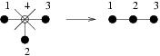
Figure 6: An internal node in a 3-node line reconnection suffers a degree increase.

∎

For further discussion, we define the following:

Degree-bounded / M-degree-bounded :

A healing algorithm is degree-bounded or M-degree-bounded if any node can increase its degree by at most $M$ in a single round of deletion and healing.

Lemma 12.

Consider a M-degree-bounded locality-aware healing algorithm used on a tree. In such a situation, deletion of a node $v$ with degree at least M+3 leads to degree increase for at least two neighbors of $v$. .

Proof.

Node $v$ has $M+3$ neighbors. By Lemma 10, the sum total of degree increase of neighbors is $M+1$, when the graph is a tree. Since one node can get a maximum degree increase of $M$, at least one node has to incur the rest of the degree increase. Thus, at least two nodes have to increase their degrees.

∎

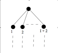
Figure 7: M+2 -ary Tree

Algorithm 2 LevelAttack: level-by-level attack on a (M+2)-ary tree

1:  Consider an (M+2)-ary tree $T$ of depth $D$ with levels numbered $0$ to $D$, the root being at level $0$.

2:  $i\leftarrow D-1$

3:  while $i\geq 0$ do

4:     for each node $v$ at level $i$ do

5:         if $v$ has $c>M+2$ children remove the excess $c-(M+2)$ nodes by deleting those with least degree increases and their subtrees by using the Prune operation, so that $v$ now has $M+2$ children.

6:        delete $v$.

7:     end for

8:     $i\leftarrow i-1$

9:  end while

Here, we introduce a new attack strategy:

LevelAttack: This strategy is described in Algorithm 2. In brief, the adversary deletes nodes one level at a time beginning one level above the leaves of a $M+2$-ary complete tree going up to the root. The reasoning behind the strategy is the following: If the adversary deletes a node of degree $M+3$ in a tree, this ensures that a degree increase of at least 1 is passed to its children. What the adversary must do is to ensure that $logn$ of these degree increases are credited to the same node.

Lemma 13.

Assume a $(M+2)-ary$ tree $T$, a degree-bounded locality-aware healing algorithm and the LevelAttack adversarial strategy. Then, when LevelAttack deleted a node at level $i$, $0<i<D$ some leaf node of the original tree increases its degree by at least $D-i$.

Proof.

The proof is by induction.

Base case: In the LevelAttack strategy, the nodes at level $D-1$ are deleted first. Thus, a deletion of a node at $D-1$ is our base case. A node at level $D-1$ has $M+3$ neighbors. By lemma 12, there is at least one leaf node that increases its degree by 1 or more. Thus, the base case holds.

Inductive step: Assume the hypothesis holds for nodes at level $i+1$. We now show that it holds for nodes at level $i$. Consider a node, say X at level $i\geq 0$ . It had $M+2$ children at level $i+1$. By the inductive hypothesis, each of these deletions led to at least one node with degree $D-(i+1)$. Moreover, $X$ is not among these $M+2$ nodes. Moreover, all of these are now neighbors of $X$, since $X$ itself was involved in each of these deletions. The Prune algorithm in step 5 retains only these $M+2$ as children of $X$. Each of these children has degree increase $D-(i+1)$ and was originally a leaf node of $T$. The adversary now deletes $X$. By lemma 12, at least one of these children incurs a degree increase.

∎

Theorem 2.

Consider any locality-aware algorithm that increases the degree of any node after an attack by at most a fixed constant. Then there exists a graph and a strategy of deletions on that graph that will force the algorithm to increase the degree of some node by at least $\log n$.

Proof.

It is sufficient to give a graph and an attack strategy such that any degree-bounded locality-aware healing algorithm will have to increase a particular node’s degree by $\log n$. Let $M$ be the constant degree increase that is the maximum that the healing algorithm can impose on any one node in the graph. Then, for a graph which is a full (M+2)-ary tree ( Figure 7), the adversary uses LevelAttack.

Consider a (M+2)-ary tree $T$ of depth $D$ with levels numbered $0$ to $D$. By lemma 13, after the last deletion in the adversary strategy, which is the deletion of the root of $T$ i.e. the node at level $0$ there is at least one node left which has a degree increase of $D$. Since $D$ is $O(logn)$, this adversary strategy achieves a degree increase of at least $O(logn)$.

∎

4 . Experiments

We carried out a number of experiments to ascertain the performance of various healing algorithms. We used a number of attack strategies to measure how different healing strategies performed with regard to degree increase and stretch, where stretch is the maximum ratio of distance increase in the healed network compared to the original network, over all pairs of nodes. Our empirical results on stretch and a heuristic for maintaining low stretch are described in Section 4.6.

4.1 . Methodology

Most of our experiments were conducted on random graphs. These graphs were generated by the Preferential attachment model proposed by Barabasi [3, 4]. The experimental approach was the following:

• For each graph size, for a particular deletion and healing strategy, repeat for 30 random instances of the graph:

  • Repeat while there are nodes in the graph:

    • delete a single node according to the deletion strategy.

    • repair according to the self-healing strategy.

    • measure the statistics (e.g. maximum change of degree for any node) for the graph.

• average the statistics for each graph size.

4.2 . Attack Strategies

The aim of the adversary is to collapse the network by trying to overload a node beyond it’s maximum capacity. There are many possible attack strategies. One strategy is to delete the node with the maximum degree. We call this the $MaxNodestrategy$. It would seem that a strategy that leads to additional burden on an already high burden node would be a good strategy. For the adversary, one good adversarial strategy is to continuously attack/delete a randomly chosen neighbor of the highest degree node in the network. We call this the $NeighborofMaxStrategy(NMS)$. This would also seem plausible as in a real network or the kind of networks we are looking at, it would be reasonable that the hubs or the high degree nodes would be more well protected and resilient to attack while their less significant neighbors should be easy to take down.

4.3 . Healing strategies

We attempted various locality-aware healing strategies, some of which are the following:

• Graph heal: On each deletion, we reconnect the neighbors of the deleted node in a binary tree regardless of whether we introduced any cycles in the graph formed by the new edges introduced for healing. This seems to be a naive algorithm since the nodes use more edges than what are required for maintaining connectivity.

• Binary tree heal: On each deletion, we reconnect the neighbors of the deleted node in a binary tree being careful not to introduce any cycles in the graph formed by the new edges introduced for healing. This is done using random IDs which can then be used to identify which tree a particular node belongs to. This is an improvement on the previous algorithm but still naive since it does not take into consideration the previous degree increase suffered by nodes during healing.

• $\mathrm{DASH}$ (degree based binary tree heal): DASH is smarter than the previous algorithms as borne out by the results of the experiments. The DASH algorithm has been earlier described in Section 2.1 and stated as Algorithm 1.

• $\mathrm{SDASH}$ (Surrogate degree based binary tree heal): (described in Section 4.6.2) A heuristic based on $\mathrm{DASH}$ that tries to keep both node degrees and path lengths small.

4.4 . Degree increase

The $NeighborofMaxStrategy$ consistently resulted in higher degree increase, hence, we report results for only this attack strategy. Our experimental results clearly show that0 $\mathrm{DASH}$ and $\mathrm{SDASH}$ are good healing strategies. It performed well against both adversary strategies. Figure 8 shows that $\mathrm{DASH}$ and $\mathrm{SDASH}$ have much lower degree increase than the other more naive strategies. Also, this degree increase was less than $\log n$, which is consistent with our theoretical results. $\mathrm{SDASH}$ has the additional nice property that it keeps path lengths small over multiple adversarial deletions.

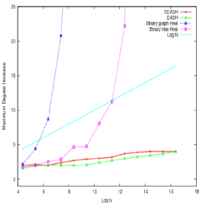
Figure 8: Maximum Degree increase: DASH vs other algorithms

4.5 . Messages

Figure 9(a) shows that the number of time a nodes $ID$ changes is less than $\log n$, as expected, for all healing strategies. Figure 9(b) shows the maximum number of messages a node sent out for the different strategies. Note that the number of messages a node sends out has to be less than or equal to the number of times a node changes ID times the degree of the node. Thus, algorithms with higher degree increase perform poorly.

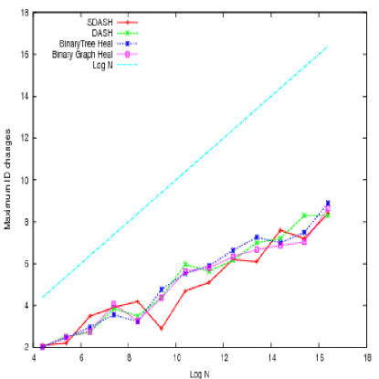
(a) ID changes for nodes

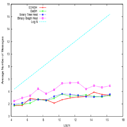
(b) Number of messages exchanged for Component(ID) information maintenance

Figure 9: ID changes and Messages exchanged per node

4.6 . Heuristics and experiments involving Stretch

4.6.1 Stretch

Stretch is an important property we would also like our self-healing algorithms to minimize. The stretch for any two nodes is the ratio between their distance in the new healed network and their distance in the original network. Stretch for the network is the maximum stretch over all pairs of nodes. Stretch is also closely related to the diameter of the network. In some sense, maintaining low degree increase and low stretch are contradictory aims since a high-degree node will lead to shorter paths and possibly lower stretch in the network.

4.6.2 $\mathrm{SDASH}$: a strategy with good empirical results

$\mathrm{SDASH}$ is an algorithm we have devised which empirically has both low degree increase and low stretch. During self-healing, we say a node surrogates if it replaces its deleted neighbor in the network. i.e. it takes all the connections of the deleted neighbor to itself. Surrogation never increases stretch since the paths never increase in length. In certain situations, it turns out that surrogation can be done without degree increase. In such situations, $\mathrm{SDASH}$ does surrogation else it simply applies $\mathrm{DASH}$. $\mathrm{SDASH}$ is described in Algorithm 3.

Algorithm 3 SDASH: Surrogate Degree-Based Self-Healing

1:  Init: for given network $G(V,E)$, Initialize each vertex with a random number $ID$ between [0,1] selected uniformly at random.

2:  while true do

3:     If a vertex $v$ is deleted, do

4:     Let $m\in UN(v,G)\cup N(v,G^{\prime})$ be the node with Maximum degree increase ($\delta$) of all nodes in $UN(v,G)\cup N(v,G^{\prime})$.

5:     if $w\in UN(v,G)\cup N(v,G^{\prime})$ and $\delta(w)+|UN(v,G)\cup N(v,G^{\prime})|-1\leq\delta(m)$  then

6:        connect all nodes in $UN(v,G)\cup N(v,G^{\prime})$ to $w$.

7:     else

8:        Nodes in $UN(v,G)\cup N(v,G^{\prime})$ are reconnected into a complete binary tree. To connect the tree, go left to right, top down, mapping nodes to the complete binary tree in increasing order of $\delta$ value.

9:     end if

10:     Let $MINID$ be the minimum $ID$ of any node in $UN(v,G)\cup N(v,G^{\prime})$. Propagate $MINID$ to all the nodes in the tree of $UN(v,G)\cup N(v,G^{\prime})$ in $G^{\prime}$. All these nodes now set their $ID$ to $MINID$.

11:  end while

As can be seen in the figures that follow, $\mathrm{SDASH}$ seems to allow a degree increase up to $O(\log n)$ and stretch up to $O(\log n)$. We are working on proving theoretical properties of this algorithm.

4.6.3 Stretch: empirical results

Figure 10 shows the performance of some of our algorithms for stretch. We determined that the $MaxNodestrategy$ is most effective for the adversary when trying to maximize stretch and so our results in Figure 10 are against that adversarial strategy. The more naive degree-control healing strategies do a good job of minimizing stretch. However, it is important to keep in mind that these more naive algorithms increase the node degrees to a point where they are unlikely to be useful for many applications. In contrast, our experiments show that $\mathrm{SDASH}$ does a good job of minimizing both stretch and degree increase.

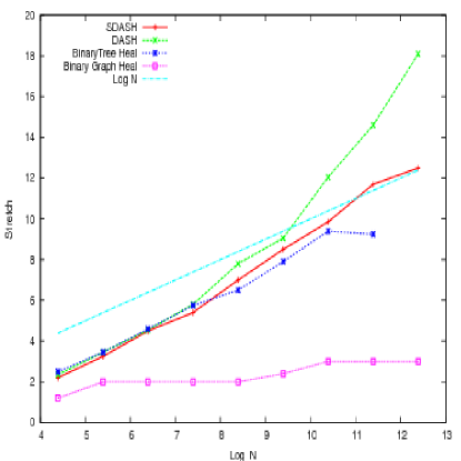
Figure 10: Stretch for various algorithms

5 . Conclusions and future work

We have studied the problem of self-healing in networks that are reconfigurable in the sense that new edges can be added to the network. We have described $\mathrm{DASH}$, a simple, efficient and localized algorithm for self-healing, that provably maintains network connectivity, even while increasing the degree of any node by no more than $O(\log n)$. We have shown that $\mathrm{DASH}$ is asymptotically optimal in terms of minimizing the degree increase of any node. Further, we have presented empirical results on power-law networks showing that $\mathrm{DASH}$ significantly outperforms the naive algorithms for this problem.

Several interesting problems remain open including the following: Can we not only maintain connectivity, but also provably ensure that lengths of shortest paths in the graph do not increase by too much? Can we remove the need for propagating IDs in order to maintain connected component information, or is such information strictly necessary to keep the degree increase small? Can we use the self-healing idea to protect invariants for combinatorial objects besides graphs? For example, can we provide algorithms to rewire a circuit so that it maintains essential functionality even when multiple gates fail?

5.1 Acknowledgments

We gratefully acknowledge the help of Iching Boman, Dr. Deepak Kapur and his class Introduction to Proofs, Logic and Term-rewriting and the UNM Computer Science Theory Seminar in writing this paper.

References

- [1] D. Andersen, H. Balakrishnan, F. Kaashoek, and R. Morris. Resilient overlay networks. SIGOPS Oper. Syst. Rev., 35(5):131–145, 2001.
- [2] V. Arak. What happened on August 16, August 2007.
- [3] A.-L. Barabasi and R. Albert. Emergence of scaling in random networks. Science, 286:509, 1999.
- [4] A.-L. Barabási and E. Bonabeau. Scale-free networks. Scientific American, pages 50–59, 2003.
- [5] I. Boman, J. Saia, C. T. Abdallah, and E. Schamiloglu. Brief announcement: Self-healing algorithms for reconfigurable networks. In Symposium on Stabilization, Safety, and Security of Distributed Systems(SSS), 2006.
- [6] I.-C. C. Boman. Algorithms for self-healing networks. M.S. Thesis, Computer Science, University of New Mexico., 2006.
- [7] R. D. Doverspike and B. Wilson. Comparison of capacity efficiency of dcs network restoration routing techniques. J. Network Syst. Manage., 2(2), 1994.
- [8] K. Fisher. Skype talks of ”perfect storm” that caused outage, clarifies blame, August 2007.
- [9] T. Frisanco. Optimal spare capacity design for various protection switchingmethods in atm networks. In Communications, 1997. ICC 97 Montreal, ’Towards the Knowledge Millennium’. 1997 IEEE International Conference on, volume 1, pages 293–298, 1997.
- [10] N. Glick. Breaking records and breaking boards. In The American Mathematical Monthly, volume 85, pages 2–26, January 1978.
- [11] S. Goel, S. Belardo, and L. Iwan. A resilient network that can operate under duress: To support communication between government agencies during crisis situations. Proceedings of the 37th Hawaii International Conference on System Sciences, 0-7695-2056-1/04:1–11, 2004.
- [12] R. R. Iraschko, M. H. MacGregor, and W. D. Grover. Optimal capacity placement for path restoration in stm or atm mesh-survivable networks. IEEE/ACM Trans. Netw., 6(3):325–336, 1998.
- [13] O. Malik. Does Skype Outage Expose P2P s Limitations?, August 2007.
- [14] G. S. Manku, M. Naor, and U. Wieder. Know thy neighbor’s neighbor: the power of lookahead in randomized p2p networks. In Proceedings of the 36th ACM Symposium on Theory of Computing (STOC), 2004.
- [15] M. Medard, S. G. Finn, and R. A. Barry. Redundant trees for preplanned recovery in arbitrary vertex-redundant or edge-redundant graphs. IEEE/ACM Transactions on Networking, 7(5):641–652, 1999.
- [16] M. Moore. Skype’s outage not a hang-up for user base, August 2007.
- [17] K. Murakami and H. S. Kim. Comparative study on restoration schemes of survivable ATM networks. In INFOCOM (1), pages 345–352, 1997.
- [18] M. Naor and U. Wieder. Know thy neighbor’s neighbor: Better routing for skip-graphs and small worlds. In The Third International Workshop on Peer-to-Peer Systems (IPTPS), 2004.
- [19] B. Ray. Skype hangs up on users, August 2007.
- [20] B. Stone. Skype: Microsoft Update Took Us Down, August 2007.
- [21] B. van Caenegem, N. Wauters, and P. Demeester. Spare capacity assignment for different restoration strategies in mesh survivable networks. In Communications, 1997. ICC 97 Montreal, ’Towards the Knowledge Millennium’. 1997 IEEE International Conference on, volume 1, pages 288–292, 1997.
- [22] Y. Xiong and L. G. Mason. Restoration strategies and spare capacity requirements in self-healing atm networks. IEEE/ACM Trans. Netw., 7(1):98–110, 1999.