Monte Carlo Simulations of Star Clusters - IV. Calibration of the Monte Carlo Code and Comparison with Observations for the Open Cluster M67

Abstract

We outline the steps needed in order to incorporate the evolution of single and binary stars into a particular Monte Carlo code for the dynamical evolution of a star cluster. We calibrate the results against $N$-body simulations, and present models for the evolution of the old open cluster M67 (which has been studied thoroughly in the literature with $N$-body techniques). The calibration is done by choosing appropriate free code parameters. We describe in particular the evolution of the binary, white dwarf and blue straggler populations, though not all channels for blue straggler formation are represented yet in our simulations. Calibrated Monte Carlo runs show good agreement with results of $N$-body simulations not only for global cluster parameters, but also for e.g. binary fraction, luminosity function and surface brightness. Comparison of Monte Carlo simulations with observational data for M67 shows that is possible to get reasonably good agreement between them. Unfortunately, because of the large statistical fluctuations of the numerical data and uncertainties in the observational data the inferred conclusions about the cluster initial conditions are not firm.

1 Introduction

The modelling of individual globular clusters has a long history (see Meylan & Heggie (1997), especially §§3 and 7.7). Much of the focus of this work is on static models such as the King model and its variants. In this kind of modelling the dynamical history of the cluster is almost irrelevant, except for the general assumption that the cluster is almost relaxed. By contrast, there have been a small number of studies based on techniques which can follow the dynamical evolution of a cluster. Most of this work has been performed with a Fokker-Planck scheme using finite differences, but also there are examples of the use of fluid and Monte Carlo methods (Tab. 1).

Table 1: Dynamical evolutionary models of individual globular clusters

Cluster	Method	Reference
47 Tuc	Fokker-Planck	Behler et al. (2003), Murphy et al. (1998)
M15	Fokker-Planck	Murphy et al. (2003, 1997, 1994), Dull et al. (1997), Grabhorn et al. (1992)
M30	Fokker-Planck	Howell, Guhathakurta & Tan (2000)
N6397	Fokker-Planck	Dull et al. (1994), Drukier (1993, 1992)
N6624	Fokker-Planck	Grabhorn et al. (1992)
$\omega$ Cen	Monte Carlo	Giersz & Heggie (2003)
M3	Moment equations	Angeletti, Dolcetta & Giannone (1980)

In the present paper we develop the Monte Carlo technique further, and apply it to a new object. The dynamical ingredients of the Monte Carlo code are essentially the same as those described in Giersz (2006), whose code embodies several features introduced by Stodołkiewicz (1986), whose code was in turn based on that originally devised by Hénon (1971). Three main features distinguish the code which is described in the present paper from that used by Giersz & Heggie (2003) in their work on $\omega$ Cen: (i) it now incorporates dynamical interactions between binary and single stars, between pairs of binaries, and interactions of three single stars resulting in the creation of new binaries, all using cross sections; (ii) it replaces the skeletal approach to stellar evolution taken from Chernoff & Weinberg (1990) by the algorithms of Hurley, Pols & Tout (2000) for the evolution of single stars, supplemented by the methods of Hurley, Tout & Pols (2002) for the internal evolution of binary stars; (iii) a better treatment of the escape process in the presence of a static tidal field according to the theory proposed by Baumgardt (2001).

There are several factors which motivate this work. Star clusters are the focus of several intensive observational campaigns (e.g. Bedin et al., 2001; Bedin, Piotto & King, 2003; Grindlay et al., 2001; Piotto et al., 2002; Kaliari et al., 2003; Kafka et al., 2004; Richer et al., 2004; Anderson et al., 2006), which are now turning to an examination of the parameters of their populations of binaries and blue stragglers (BS). Dynamical models are needed for the design and interpretation of observational programmes: how is the period distribution and the spatial distribution of binaries affected by dynamical evolution? Another problem is the abundance and spatial distribution of blue stragglers, which can only be answered by a technique which follows simultaneously both their dynamics and internal evolution. While $N$-body techniques may ultimately be the method of choice for such studies, systems with the size of a globular cluster are likely to remain beyond reach for some years, simply because of the number of stars and the population of binaries. After all, it is only recently that the “hardest” open clusters have been modelled at the necessary level of sophistication, and even then the typical simulation takes one month (Hurley et al., 2005). These authors focused on the old open cluster M67, which has been chosen by the MODEST international collaboration (MOdelling DEnse STellar systems) (Sills et al., 2003) as a target cluster for comparison between observations and various techniques of numerical simulation. We also focus on this cluster, partly for the purpose of refining our calibration of the Monte Carlo method.

This paper begins in Sec.2 with a summary of the features which have been added to the Monte Carlo scheme. We also show there how we calibrate the Monte Carlo technique with $N$-body simulations. Next (Sec. 3) we apply the technique to construct a dynamical evolutionary model of the old open cluster M67, and compare our results with observations. We give predictions for the initial parameters of the old open cluster M67. The final section summarises our conclusions, and discusses some of the main limitations of our models.

2 Technique

2.1 Coding of binary- and single-star evolution

From the dynamical point of view our Monte Carlo code is almost exactly as described in Giersz (2006). In this technique a star cluster is treated as a collection of spherical shells, each one representing a single star with a certain energy and angular momentum. Neighbouring shells are allowed to interact and exchange energy and angular momentum at a rate determined by the theory of relaxation. Escapers are removed according to a prescription which mimics the effect of a tide. Shells corresponding to binary stars also interact with single stars, and other binary stars, at rates determined by cross sections drawn from the literature (Giersz, 2001). The only dynamical alterations deal with tightly bound subsystems, which often arise in systems with a large mass range (e.g. those including both stellar-mass black holes and stars at the hydrogen-burning limit of the main sequence).

The introduction of stellar and binary evolution has been greatly facilitated by the development of the “McScatter” interface (Heggie, Portegies Zwart & Hurley, 2006), which provides subroutines for initialising the stellar evolution of single and binary stars, and for retrieving the results of subsequent evolution, mass loss, merging of binary components, etc. At present two such packages for stellar evolution can be employed. One of these is SeBa (Portegies Zwart & Verbunt, 1996), which is incorporated within the STARLAB environment (Hut, 2003). The other is referred to as “BSE” (binary star evolution), and is based on the extensive formulae for the evolution of single stars of a range of metallicities given by Hurley, Pols & Tout (2000), along with the treatment of binaries presented by Hurley, Tout & Pols (2002). Most of our effort has been conducted with BSE, partly to minimise any development problems with mixed-language programming, and partly because SeBa is at present restricted to solar metallicity, whereas our interest is mainly directed to globular clusters. Generally speaking, the use of the McScatter interface poses few problems:

1. There was one instance of a named common block in BSE which by coincidence was the same as the name of one common block in the Monte Carlo code; a change of name in the Monte Carlo code was sufficient cure.

2. The enumeration of stars requires care. Although it is not clear from the interface, the numerical identity of each binary determines the numerical identity of the two single stars from which it is composed, and it is important that the numerical identities of all single stars (both binary components and those which are genuinely single) are different.

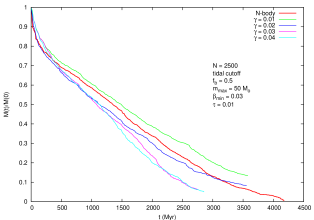
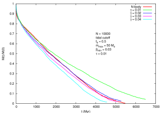
Figure 1: Comparison of $N$-body and Monte Carlo simulations for models with tidal cutoff. The mass (normalised by its initial value) is given as a function of time. The initial conditions are given in Tab. 2 and described in the figures. The value of $N$ referred to is $N_{s}+N_{b}$, but this differs from the total number of particles ($N_{s}+2N_{b}$). The $N$-body model is the heavy continuous line, and the others are Monte-Carlo simulations with (from the left) $\gamma=0.04,0.03,0.02,0.01$.

During a time step of the Monte Carlo code, the changes caused by relaxation and dynamical interactions between binaries and single stars are performed, and then the stellar evolution of all stars and binaries is updated. The associated loss of mass (if any) is incorporated into the data for each star and binary in the Monte Carlo code, and any mergers are dealt with by altering the numbers of single and binary stars and adjusting the parameters of the bodies affected.

2.2 Calibration

In a Monte Carlo simulation it is usual to adopt units such that the constant of gravitation, the initial total mass and the initial virial radius are 1. In order to incorporate stellar evolution into a Monte Carlo simulation, dimensional values for the initial total mass and virial radius (or equivalent) must be specified, and then the unit of time in the Monte Carlo code (which is essentially a relaxation time) is expressible dimensionally with a factor proportional to $N/\log(\gamma N)$, where $\gamma$ is a constant and $N$ is the number of stars in the system. While the value of $\gamma$ is rather well known for the case of single stars of equal mass, i.e. $\gamma=0.11$ approximately (Giersz & Heggie, 1994; Joshi, Rasio & Portegies Zwart, 2000), the case of unequal masses with a population of primordial binaries has been studied much less. On analytical grounds Hénon (1975) gave a formula which, by way of example, yields a value $\gamma=0.007$ approximately for a mass function for single stars of the form $dN\propto m^{-2}dm$, over a range in which the mass ratio between the maximum and minimum mass is $500:1$. This theory also implies that the value depends on the mass ratio, which changes through stellar evolution. Giersz & Heggie (1996) found a value $\gamma\simeq 0.015$ for a power-law mass function of index $-2.5$ and a smaller mass range of $37.5:1$, by means of intercomparison of $N$-body simulations, and somewhat larger values from Hénon’s formula or from comparison with isotropic Fokker-Planck models.

Here we adopt a pragmatic approach, comparing Monte Carlo and $N$-body models with identical initial conditions. These are summarised in Tab. 2, where the tidal radius refers to a tidal cutoff (or, for the $N$-body models discussed from Sec.2.2.2 onwards, a tidal field). It is necessary to carry out this comparison for at least two values of $N$. If we were to determine $\gamma$ from a single value of $N$, it might be that this value simply obscures some systematic problem with the Monte Carlo code, and would fail for a different value of $N$. Modest values of $N$ are better for this purpose, as the $N$-dependence of the Coulomb logarithm becomes weaker as $N$ increases. We study cases with $N=N_{s}+2N_{b}=3750$ and $15000$, where $N_{s},N_{b}$ are the initial numbers of single and binary stars, respectively.

The Monte Carlo code free parameters are as follows: (i)   $\gamma$, (ii)   $\beta_{min}$, minimum value of the deflection angle (Giersz, 1998), (iii)   $\tau$, the overall time step and (iv)  $\alpha$, see for the definition Sec. 2.2.2.

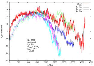
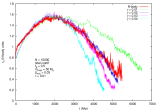
Figure 2: Comparison of the evolution of the half-mass radius in $N$-body and Monte Carlo simulations for models with tidal cutoff. The initial conditions are given in Tab. 2 and described in the figures. The value of $N$ referred to is $N_{s}+N_{b}$. The $N$-body model is the heavy continuous line, and the others are Monte-Carlo simulations with (from the left, at late times) $\gamma=0.04,0.03,0.02,0.01$. The mismatch at early times in the upper panel is discussed in 2.2.2.

Table 2: Initial conditions of calibration runs

$N_{s}+2N_{b}$	$3750$ ($15000$)
Initial model	Plummer
Initial tidal radius	$30$pc ($30$pc)
Initial half-mass radius	$3$pc ($3$pc)
Initial mass function	Kroupa, Tout & Gilmore (1993)
	with $\alpha_{1}=1.3$, mass range
	between $0.1M_{\odot}$ and $50M_{\odot}$
Binary fraction	$N_{s}/(N_{s}+N_{b})=0.5$
Binary eccentricities	$f(e)=2e$
Binary semi-major axes	Uniformly distributed in the
	logarithm in the range
	$2(R_{1}+R_{2})$ to 50AU
Run time (Monte Carlo)	0.4 min (3 min)
Run time (NBODY4 with	41 min (1400 min)
GRAPE6Af)

Notes: where two values are given, the first value refers to runs with $N_{s}+2N_{b}=3750$, the second (in brackets) to those with $N_{s}+2N_{b}=15000$. The timings are on a 3GHz PC ($N$-body) and AMD Opetron 242 (Monte Carlo).

2.2.1 Models with tidal cutoff

First, we concentrated on calibration of Monte Carlo models for which the influence of the tidal field of a parent galaxy is characterised by the tidal energy cutoff - all stars which have energy larger than $E_{t_{c}}=-GM/r_{t}$ are immediately removed from the system – $M$ is the total mass and $r_{t}$ is the tidal radius. The comparison of the evolution of the mass with time (Fig. 1) suggests that a value just about $\gamma=0.02$ is an appropriate choice (especially for an age of order a few Gyr, as in M67).

Apart from mass, the other fundamental measure of a cluster is its radius, and the same comparison for the half-mass radius ($r_{h}$) is presented in Fig. 2. It is however, much less discriminating of the appropriate value of $\gamma$, particularly for $N=2500$. A comparison of the two panels also suggests caution in applying the Monte Carlo method to a single system with $N\mathrel{\raise 1.29167pt\hbox{$<$}\mkern-14.0mu\lower 2.58334pt\hbox{$\sim$}}10^{3}$, because of the increasing role of statistical fluctuations.

To properly assess the inferred values of the free parameters of the Monte Carlo code it is important to check the intrinsic statistical fluctuation of the code.

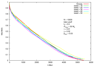
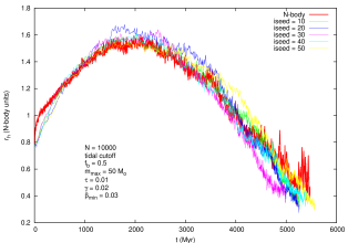
Figure 3: Comparison of the evolution of the total mass and half-mass radius in $N$-body and Monte Carlo simulations for models with tidal cutoff. The initial conditions are given in Tab. 2 and described in the figures. The $N$-body model is the heavy continuous line, and the others are Monte-Carlo simulations with different initial random number sequence $iseed=10,20,30,40,50$.

As can be seen from Fig. 3 the spread between models with exactly the same parameters, but with different initial random number sequence (iseed), is substantial, even for $N=15000$. This spread is even larger for $N=2500$, as can be expected from theory. The spread between results with different $\beta_{min}$ and $\tau$ is well inside the spread connected with different iseed. Only the spread between models with different $\gamma$ is larger that the one connected with different iseed. The best values of the free code parameters are: $\gamma=0.2$, $\beta=0.03$ and $\tau=0.01$.

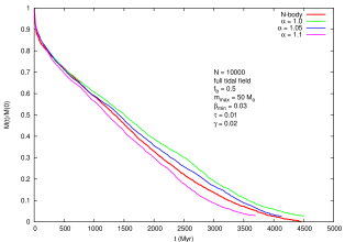
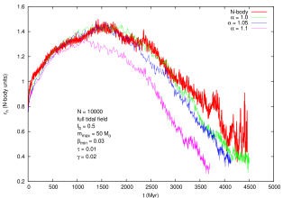
Figure 4: Comparison of the evolution of the total mass and the half-mass radius in $N$-body and Monte Carlo simulations for models with full tidal field. The initial conditions are given in Tab. 2 and described in the figures. The $N$-body model is the heavy continuous line, and the others are Monte-Carlo simulations with (from the right) $\alpha=1.0,1.05,1.1$.

2.2.2 Models with full tidal field

The process of escape from a cluster in a steady tidal field is extremely complicated. Some stars which fulfil the energy criterion (binding energy of the star greater than the critical energy $E_{t_{f}}=-1.5(GM/r_{t})$, see Spitzer (1987)) can still be trapped inside the potential well. Those stars can be scattered back to lower energy before they escape from the system. As was pointed out by Baumgardt (2001) these mechanisms cause the cluster lifetime to scale nonlinearly with relaxation time, in contrast with what would be expected from the standard theory. The efficiency of these effects decreases as the number of stars increases. To account for this in the Monte Carlo code an additional free parameter was introduced according to the theory presented by Baumgardt (2001). The critical energy for escaping stars was approximated by: $E_{t_{f}}=-\alpha(GM/r_{t})$, where $\alpha=1.5-a(ln(\gamma N)/N)^{1/4}$. Thus the effective tidal radius for Monte Carlo simulations is $r_{t_{eff}}=r_{t}/\alpha$ and it is smaller than $r_{t}$. This leads to the result that for Monte Carlo simulations a system is slightly too concentrated compared to $N$-body simulations, but the evolution of the total mass is well reproduced, as well as the scaling of the dissolution time with $N$.

Fig. 4 shows the evolution of the total mass and the half-mass radius for different $\alpha$ for $N=10000$. The other free parameters for the case of a full tidal field are the same as for the tidal cutoff case: $\gamma=0.02$, $\tau=0.01$ and $\beta_{min}=0.03$. As can be seen by comparing Fig.5 (lower two panels) with Fig.3 (top panel), again the spread between models with different $\beta_{min}$ and $\tau$ is well inside the spread connected with different iseed. The statistical spread also does not substantially interfere with the determination of $\alpha$ and $\gamma$ (see Fig.5 (top panel) for $\gamma$).

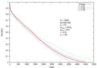
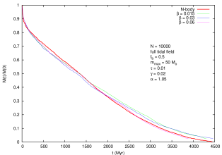
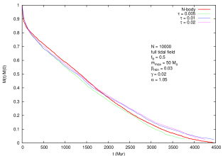
Figure 5: Comparison of the evolution of the total mass in $N$-body and Monte Carlo simulations for models with full tidal field. The initial conditions are given in Tab. 2 and described in the figures. The $N$-body model is the heavy continuous line, and the others are Monte-Carlo simulations with (from the left) $\gamma=0.03,0.02,0.01$ (top), (from the ) $\beta=0.06,0.03,0.015$ (middle), and (from the right) $\tau=0.02,0.01,0.005$ (bottom).

As can be seen in Fig. 4 (lower panel) the evolution of $r_{h}$ up to time about 0.5 Gyr is slightly too slow in comparison to $N$-body results. (This effect is even more pronounced for smaller $N$: see Fig.2, top panel.) This behaviour is connected with the way in which the effect of stellar mass loss is fed in to the cluster. In the Monte Carlo model the stellar evolution mass loss is postponed until the end of the overall time step, usually several Myr. So, for the most massive stars the stellar evolution can be substantially delayed and the cluster expands slower. In Fig. 6 the evolution of $r_{h}$ is presented for different models in which the overall time step was reduced by factor of two up to a certain time, $s$. It is clear that reduction of the overall time step in the phases of cluster evolution in which the most massive stars end their evolution helps to bring the Monte Carlo results close to the $N$-body ones. In later phases of cluster evolution, in which the time-scale of stellar evolution becomes larger than the half-mass relaxation time, the evolution does not depend systematically on the chosen overall time step. (In the simulations used in the determination of the free code parameters the adopted overall time step was a compromise between accuracy and speed.)

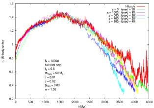
Figure 6: Comparison of the evolution of the half-mass radius in $N$-body and Monte Carlo simulations for models with a full tidal field. The initial conditions are given in Tab. 2 and described in the figures. The $N$-body model is the heavy continuous line, and the others are Monte-Carlo simulations with different time, $s$, up to which the overall time step is half of the standard one. The model with $s=100$ has two different statistical realisations with $iseed=20,40$. Note that some curves are overprinted (and hence invisible) at early times.

As can be seen in Figs. 7, 8, 9 the Monte Carlo code can reproduce $N$-body simulations not only in respect of the global parameters of the system, but also in respect of properties connected with binary activity. Despite the fact that the total number of binaries in the system and the binary fraction agree quite well with $N$-body simulations, the total binding energy is substantially too high for the Monte Carlo simulations. This is connected with the fact that the present Monte Carlo simulations cannot follow 3- and 4-body interactions directly as the $N$-body code does. Binaries can only harden or dissolve. Therefore much of the complexity of binary dynamical interactions is missing in the present Monte Carlo simulations.

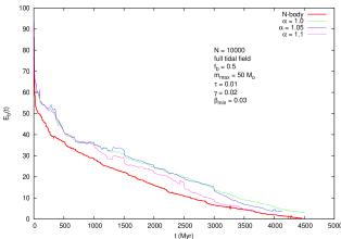
Figure 7: Comparison of the evolution of the binary binding energy in $N$-body and Monte Carlo simulations for models with full tidal field. The initial conditions are given in Tab. 2 and described in the figures. The $N$-body model is the heavy continuous line, and the others are Monte-Carlo simulations with $\alpha=1.1,1.05,1.0$.

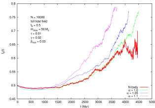
Figure 8: Comparison of the evolution of the binary fraction in $N$-body and Monte Carlo simulations for models with full tidal field. The initial conditions are given in Tab. 2 and described in the figures. The $N$-body model is the heavy continuous line, and the others are Monte-Carlo simulations with $\alpha=1.1,1.05,1.0$.

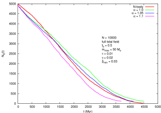
Figure 9: Comparison of the evolution of the number of binaries in $N$-body and Monte Carlo simulations for models with full tidal field. The initial conditions are given in Tab. 2 and described in the figures. The $N$-body model is the heavy continuous line, and the others are Monte-Carlo simulations with $\alpha=1.1,1.05,1.0$.

In Fig. 10 is shown the number of collisions as a function of time for the Monte Carlo and $N$-body models. The collisions are mainly connected with binary mergers due to stellar evolution or dynamical binary interactions. There are only a few direct physical collisions between single stars. Up to time about 1.5 Gyr both models give similar results, and then the $N$-body model shows a larger number of collisions than the Monte Carlo model. Again this can be attributed to the fact that in the Monte Carlo simulations the complex dynamical binary interactions are not followed. In the Monte Carlo code a binary can only coallesce if, after the dynamical interaction, the periastron distance is smaller than the sum of the stellar radii. In the $N$-body code binary coallescence occurs if, during the interaction, the distance between two stars is smaller than the sum of their radii. Definitely the latter can happen more frequently, in the case of strong interactions such as prolonged resonances (temporary capture). When most collision events are connected with the stellar evolution of nearly isolated binaries, then both models agree.

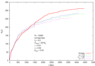
Figure 10: Comparison of the evolution of the number of collisions in $N$-body and Monte Carlo simulations for models with full tidal field. The initial conditions are given in Tab. 2 and described in the figures. The $N$-body model is the heavy continuous line, and the others are Monte-Carlo simulations with $\alpha=1.1,1.05,1.0$.

2.2.3 Model of M67

The old open cluster M67 is an ideal testing ground for modelling the interactions between dynamical and stellar evolution. It has a substantial population of blue stragglers, which are almost certainly the product of stellar collisions, or mergers within primordial binaries. Also, it is small enough that its entire life history can be modelled with $N$-body techniques (Hurley et al., 2005), though this has become possible only within the last few years: though its present mass (of order $2000M_{\odot}$) makes it seem an easy target for simulation, its initial mass is likely to have been much higher (Tab. 3). This table also specifies the other initial parameters for our model, which closely follow the prescription of Hurley et al. (2005). The initial value of the tidal radius is determined by scaling the value in their model at 4Gyr to the initial mass of our model.

Table 3: Initial conditions for M67

$N_{s}+N_{b}$	$24000$
M(0)	$1.904\times 10^{4}M_{\odot}$
Initial model	Plummer
Initial tidal radius	$32.2$pc
Initial mass function	Kroupa, Tout & Gilmore (1993)
	with $\alpha_{1}=1.3$
IMF of binaries	Kroupa, Gilmore & Tout (1991), eq.(1)
Binary fraction	$N_{s}/(N_{s}+N_{b})=0.5$
Binary eccentricities	$f(e)=2e$
Binary semi-major axes	Uniformly distributed in the logarithm
	in the range $2(R_{1}+R_{2})$ to $50$AU
Run time (Monte Carlo)	7 min
Run time (NBODY6)	1 month

The data from $N$-body simulations of M67 (Hurley et al., 2005) were used to calibrate the last remaining parameter of the Monte Carlo code, namely $\alpha$. The inferred formula is $\alpha=1.5-3.0(ln(\gamma N)/N)^{1/4}$. The comparison of results from $N$-body and Monte Carlo simulations for M67 confirmed the values of $\gamma$, $\tau$ and $\beta_{min}$ found for smaller $N$ systems.

Table 4: Monte Carlo and $N$-body results for M67 at 4 Gyr

	$N$-body (Hurley et al., 2005)	This work
$M/M_{\odot}$	2037	1984
$f_{b}$	0.60	0.59
$r_{t}$ $pc^{-1}$	15.2	15.1
$r_{h}$ $pc^{-1}$	3.80	3.03
$M_{L}/M_{\odot}$	1488	1219
$M_{L10}/M_{\odot}$	1342	1205
$r_{h,L10}$ $pc^{-1}$	2.70	2.67

L – stars with mass above $0.5M_{\odot}$ and burning nuclear fuel

L10 – the same as L but for stars contained within 10 pc

The results of a comparison are summarised in Tab. 4. Taking into account the intrinsic statistical fluctuations of both methods the results presented in Tab. 4 show reasonably good agreement. At the time of 4 Gyr, when the comparison was done, both models consist of only a small fraction of the initial number of stars, making fluctuations even more important. The values of the half-mass radius $r_{h}$ suggest that the Monte Carlo model is slightly too concentrated by comparison with the $N$-body model. This, however, can be attributed to the treatment of the tide (Sec.2.2.2), which leads to a smaller effective tidal radius than the tidal radius inferred from $N$-body simulations. Additionally, in $N$-body simulations, stars are considered as escapers only if their distance from the cluster centre is larger than $2r_{t}$ (Hurley et al., 2005). The mass outside $r_{t}$ is about $100M_{\odot}$ (see Fig.11), which is small compared to the total cluster mass at any time, but nevertheless leads to slightly too large a half-mass radius. Compared to $N$-body simulations, the values shown by the Monte Carlo simulations for the luminous mass $M_{L}$ and the luminous mass inside 10 pc distance from the centre $M_{L10}$ are too low. (The luminous mass is the mass of all stars with mass above $0.5M_{\odot}$ and burning nuclear fuel (Hurley et al., 2005)). The reasons for this disagreement are unclear, but it is partly attributable to the smaller total mass of the Monte Carlo model, and balanced by the somewhat larger total mass in white dwarfs (see below). Note, however, that the lower effective tidal radius, $r_{t_{eff}}$, in the Monte Carlo model forces most stars to be confined inside 10 pc. Therefore $M_{L}$ and $M_{L10}$ are practically identical for the Monte Carlo simulations. Furthermore, the mismatch between the two models is much smaller inside 10pc, which suggests that the reason for the disagreement in $M_{L}$ concerns mainly large radii.

The spatial distributions of mass for the Monte Carlo and $N$-body models are illustrated in Fig. 11. There are only 4 blue stragglers in the model, compared with 20 in the $N$-body model. Agreement is not expected, because our model excludes one of the main channels for blue straggler production, i.e. collisions during resonant encounters. Despite the large difference in the number of blue stragglers present in both models, their mass distributions are very similar. Blue stragglers are more centrally concentrated then other luminous object in the cluster. The comparison with the $N$-body model is qualitatively satisfactory, but quantitatively reflects the larger half-mass radius and larger effective tidal radius in the $N$-body model.

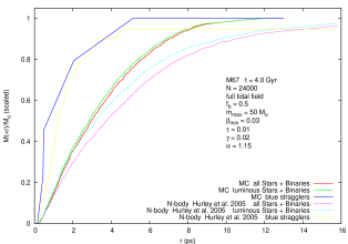
Figure 11: Mass profiles of the Monte Carlo and $N$-body models of M67 at 4Gyr, scaled by the total mass involved in constructing the profile; from the right all mass, luminous mass (as defined in the text) and blue stragglers. The initial conditions are given in Tab. 3 and described in the figure.

Comparisons of the time-evolution of the number-density within the core and half-mass radii for Monte Carlo and $N$-body models are presented in Fig. 12. Agreement between the two models is quite satisfactory. The observed difference can be attributed to two factors:

1. different definitions of the core radius are used in the two models. In the Monte Carlo model the core radius is defined according to equation 1-34 in Spitzer (1987) and in the $N$-body model from a density-weighted radius (Casertano & Hut, 1985);

2. the Monte Carlo model is more centrally concentrated than the $N$-body model because of the smaller effective tidal radius $r_{t_{eff}}$.

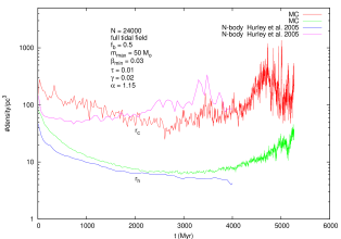
Figure 12: Number density within the core and half-mass radii of the Monte Carlo and $N$-body models of M67, as a function of time. The initial conditions are given in Tab. 3 and described in the figure.

A comparison of the projected number density of luminous stars above $0.8M_{\odot}$ for the Monte Carlo and $N$-body simulations and from observations (Bica & Bonatto (2005) as quoted in Hurley et al. (2005)) is presented in Fig. 13. This confirms the conclusions reached so far: the overall density of the Monte Carlo model is slightly larger than that of the $N$-body model and the half-mass radius of the Monte Carlo model is too small. Both models exceed the observed surface density in the central part of the system but underpredict it in the outer halo. These regions require separate discussion:

1. The higher observational value at large radii suggests contamination of the observed field by stars which are not members of the cluster. Indeed, the data quoted in Hurley et al. (2005) are not corrected for the background density of stars. We also have not corrected the data for the background, in order to analyse the simulation data in the same way as in Hurley et al. (2005) (see Fig. 7 there). (We consider the effect of the background in Sec.3).

2. It is possible that the observational value at small radii could be lowered if it were supposed that the observations are not fully corrected for the large binary fraction in the core. Furthermore, as can be seen from the numerical simulations, the surface density is lower if only luminous stars are taken into account. So, corrections for a low-luminosity cutoff and unresolved binaries can help to bring observation and simulation closer. However, we should not expect a large correction factor for contamination, because of the high latitude of M67.

This discussion of the centre of M67 suggests that probably only some changes in the initial model of M67 can bring both observations and simulations into agreement, and we consider this in Sec.3. (That was not our intention in the present section, where our aim is to check that the Monte Carlo code can produce results consistent with the $N$-body model for a realistic cluster model.)

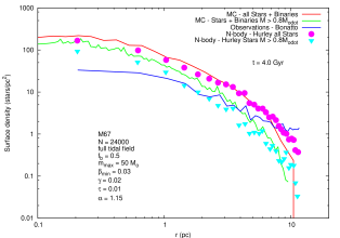
Figure 13: Profile of the projected number density of all luminous stars and binaries and luminous stars above $0.8M_{\odot}$, compared with the observations of Bonatto & Bica (extracted from Hurley et al. (2005, Fig.7)) and $N$-body simulations at 4 Gyr. The initial conditions are given in Tab. 3 and described in the figure.

In Fig. 14 the surface brightness profiles for the Monte Carlo and $N$-body models are presented. To construct these surface brightness profiles all stars and binaries were used. The data are very noisy, particularly for the $N$-body simulation. The agreement between the two models is reasonably good. Again the conclusion reached before are confirmed. The surface brightness in the central parts of the system is slightly larger for the Monte Carlo model than that of $N$-body model and outside in the cluster halo the surface brightness is larger for the $N$-body model. The latter is again connected with the effective tidal radius for the Monte Carlo code which is smaller than the nominal tidal radius for the two models. Its effects are particularly clear in Fig.13.

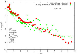
Figure 14: Surface brightness profile of all luminous stars and binaries for the Monte Carlo and $N$-body simulations at 4 Gyr. The initial conditions are given in Tab. 3 and described in the figure.

A form of colour-magnitude diagram is shown in Fig. 15, which can be compared with Fig.10 of Hurley et al. (2005). The resemblance is qualitatively satisfactory, except for the relative paucity, already referred to, of blue stragglers in the Monte Carlo model, and the shortness of the sequence of blue stragglers, compared to the $N$-body model.

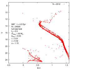
Figure 15: Colour-magnitude diagram at 4 Gyr for Monte Carlo simulation. The initial conditions are given in Tab. 3 and described in the figure.

Hurley et al. (2005) discuss the different exotic populations of their model at some length. As already stated in connection with the blue straggler population, however, our model lacks important processes for the formation of such objects. Therefore we confine attention to more normal populations, namely white dwarfs. The mass fraction of white dwarfs is $0.18$, slightly larger than the value of $0.15$ given by Hurley et al. (2005). Therefore the total mass in white dwarfs is larger in the Monte Carlo model by about 60$M_{\odot}$. In particular the white dwarf fraction in the central part of the system is larger for the Monte Carlo model than for the $N$-body model (Fig. 16). The spatial distributions of white dwarfs are similar in the two models. The maximum lies around 6 – 8 pc, and is more pronounced in the $N$-body model; in the Monte Carlo model the profile could be flat (within fluctuations) below this range of radii. The half-mass radius of the white dwarfs is 2.73 pc, much bigger than the value of 0.6 pc reported by Hurley et al. (2005); we believe their value may be in error.

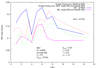
Figure 16: Mass fraction of white dwarfs as a function of radius for Monte Carlo and $N$-body models at 4 Gyr. The results are for all WDs and only single WDs and double WDs. The initial conditions are given in Tab. 3 and described in the figure.

For single main sequence stars we present in Fig. 17 the luminosity functions for the Monte Carlo and $N$-body models for times 0 Gyr and 4 Gyr. The luminosity functions for time 0 Gyr agree quite well for the two models. Only for very bright stars, $V<10$ mag, can one observe noticeable differences. They can be attributed to statistical fluctuations connected with different realisations of the initial model. For 4 Gyr our Monte Carlo result misses significant numbers of stars at the high-luminosity end of the distribution, which are found in the $N$-body simulation and which Hurley et al. (2005) attribute to collisions; as already stated in our discussion of blue stragglers, important channels for the formation of such stars are missing at present in our model. For the low mass end of the luminosity function the two models agree reasonably well.

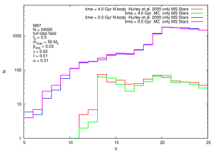
Figure 17: Luminosity function of single main sequence stars for Monte Carlo and $N$-body models at 0 Gyr and 4 Gyr. The initial conditions are given in Tab. 3 and described in the figure.

Finally, the comparison between observations (Montgomery, Marschall & Janes, 1993) and the Monte Carlo simulations for the luminosity function is presented in Fig. 18. The luminosity function was normalised by the number of stars with luminosity $V<15.5$ mag. In the figure are shown the luminosity functions for only main sequence stars, only main sequence binaries, and all main sequence stars and binaries (for the Monte Carlo model) and for main sequence stars and binaries (observations). It is clear that the simulations do not agree with the observations. The luminosity function for the Monte Carlo model is too low at the high-luminosity end, too high at the low-luminosity end and too high near the main sequence turn-off ($V=13$ mag). The drop in the luminosity function of the Monte Carlo model at the high-luminosity end can be attributed to an underproduction of blue stragglers in the Monte Carlo model comparable to observations. The excessive luminosity function at the low-luminosity end and around the main sequence turn off cannot be so easily explained. Even though observational issues may be relevant at the faint end (Sec.3), some of these mismatches suggest that the initial model of M67 is wrong and some refinement is needed. Because the Monte Carlo model agrees so well with the $N$-body model (Fig.17), similar conclusions may be reached for a comparison of the $N$-body model with observed luminosity function, except for the region occupied by blue stragglers.

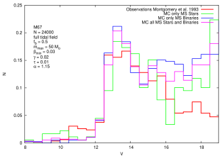
Figure 18: Comparison of the luminosity function for the Monte Carlo model at 4 Gyr and observations (Montgomery at al. 1993), for main sequence stars only, binaries only and both main sequence stars and binaries. The initial conditions are given in Tab. 3 and described in the figure. Note that all curves are normalised separately.

In this section it has been shown that the Monte Carlo code is able to follow the evolution of a realistic star cluster model at a similar level of complexity to that of the $N$-body code. The data provided by the code is as detailed as for the $N$-body code and can be used for comparison with many kinds of observational data. The next section will be devoted to further Monte Carlo modeling of the old open cluster M67 in order to improve the match with its observational properties and find possible initial conditions for this cluster.

3 Refinement of the M67 model

As was shown in the previous subsection (see Sec. 2.2.3) the model of M67 proposed by Hurley et al. (2005), whether one uses an $N$-body code or a Monte Carlo code, shows significant disagreement with such observational properties of the cluster as the luminosity function and the surface density profile. Other observational data about M67 are summarised in Hurley et al. (2005) and listed in Tab. 5. Generally, however, the structural cluster parameters are not well known, and have been derived from more basic data by some model-dependent analysis. Therefore we prefer to compare with the observational data as directly as possible.

Table 5: Properties of M67 ^a

Distance from Sun	870 pc
Absolute distance modulus b	9.44
Distance from GC	6.8 – 9.1 kpc
Orbit eccentricity	0.14
Luminous mass	$\sim 1000M_{\odot}$
Core radius	1.2 pc
Tidal radius	$>11.4$ pc
Half-mass radius c	$\sim 3.0$ pc
Binary fraction	$\sim 50\%$
Z	$\sim 0.0$
Age	$\sim 4$ Gyr
$A_{V}=3.25E(B-V)$	0.16

^a References are given in Hurley et al. (2005)

^b (Montgomery, Marschall & Janes, 1993); used in the calculation of the luminosity function of of the model

^c For main sequence stars with masses $\geq 0.87M_{\odot}$ and within 10 pc

The observational data we shall use for comparison with the results of Monte Carlo simulations are: (i) the luminosity function - (Montgomery, Marschall & Janes, 1993), and (ii) the surface density profile - (Bonatto & Bica, 2003; Bica & Bonatto, 2005). Unfortunately, the observational data for the surface density profile also seem very uncertain, even though they were collected by 2MASS (Two Micron All Sky Survey); they differ by a factor larger than 1.5. In all figures in which the surface density profiles will be presented there are two observational curves: (i) - (Bica & Bonatto, 2005) (bottom), corrected for the background density at the level of $0.73$ stars arcmin^-2, which was estimated at the distance about $25$ arcmin, and (ii) - (Bonatto & Bica, 2003) (top), corrected for the background density at the level of $4$ stars pc^-2, which was estimated at the limiting radius about $9$ pc.

The model of M67 presented in the previous section had three problems: (i) it was too dense, (ii) it produced too flat a luminosity function for dim stars, and (iii) it contained too many stars around the main sequence turn off. If we take the observations at face value, to bring the model into better agreement with observation it has to either lose more of its less massive stars, or else contain smaller numbers of those stars initially. Additionally, it has to have some property such as initial mass segregation or stronger energy generation in order to show a smaller concentration at the present day. We now describe the parameter space which we explored in order to improve the model.

The free parameters of the initial models are: (i)   $N$, number of objects (stars and binaries), which we explored in the range between 22000 and 40000, (ii)   $f_{b}$, binary fraction, in the range between 0.4 and 0.7, (iii)   $r_{t}$, tidal radius, between 30 and 38 pc, (iv)   $r_{t}/r_{h}$, i.e. the ratio between the tidal and half-mass radii, between 6 and 12, and (v)  $\alpha_{IMF}$, the power-law index of the low-mass part of the initial mass function (IMF), between 0.1 and 1.3. (The canonical value is $\alpha_{IMF}=1.3$ (Kroupa, 2007)). Over 135 models of the old open cluster M67 were run. We did not carry out this exploration very systematically; rather on the basis of inspection of the results, the parameters of the next set of new models were chosen.

Unfortunately, there is no single model which can reproduce the observational properties of the cluster. Instead, there are several models which can equally well produce a reasonable fit to the observations (Figs. 19, 20, 21, 22, 23)

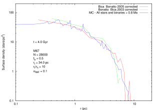
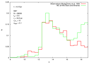
Figure 19: Comparison of the surface density profile and luminosity function for the Monte Carlo model for $\alpha_{IMF}=0.1$ and observations. The initial model parameters are described in the figures. The observational data is described in the text

In general from very low values of $\alpha_{IMF}$, i.e. 0.1, up to the canonical value, 1.3, the agreement with observations is reasonably good. For some models the luminosity function is modelled better, while for others the surface density profile is better. The initial parameters of the best models and the parameters at 4 Gyr are summarised in Tab. 6. The other model parameters are close to those chosen by Hurley et al. (2005). The free parameters of the Monte Carlo code are exactly as determined in the previous Sections.

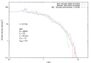
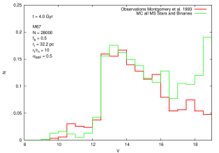
Figure 20: Comparison of the surface density profile and luminosity function for the Monte Carlo model for $\alpha_{IMF}=0.5$ and observations. The initial model parameters are described in the figures. The observational data is described in the text

Table 6: Initial parameters, and data at time 4 Gyr, for some models of M67

	t = 0						t = 4 Gyr						Figure
Model	N	$M(M_{\odot})$	$r_{t}$(pc)	$r_{t}/r_{h}$	$\alpha_{IMF}$	$f_{b}$	$M(M_{\odot})$	$M_{L10}(M_{\odot})$	$r_{t}$	$r_{h}$(pc)	$r_{hl10}$(pc)	$f_{b}$
I	28000	28747.2	34.0	10	0.1	0.5	1730.6	1007.6	13.3	3.3	3.1	0.54	19
II	28000	26329.2	32.2	10	0.5	0.5	2065.4	1215.0	13.8	3.2	3.1	0.53	20
III	32000	29228.5	32.0	10	0.7	0.4	1488.8	908.4	11.9	3.1	3.0	0.50	21
IV	32000a	28167.3	32.0	10	0.7	0.4	2815.2	1588.9	14.8	3.6	3.3	0.46	24
V	28000	26806.7	32.2	10	0.9	0.6	1587.2	992.8	12.5	2.6	2.5	0.64	22
VI	28000	24195.6	33.0	10	1.3	0.5	1799.1	1078.7	13.9	3.0	2.8	0.60	23

L10 – stars with mass above $0.5M_{\odot}$, burning nuclear fuel and contained within 10 pc

^a model with different initial realisation of the sequence of random numbers. All other model parameters are the same as for the model above.

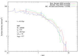
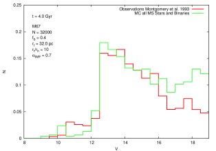
Figure 21: Comparison of the surface density profile and luminosity function for the Monte Carlo model for $\alpha_{IMF}=0.7$ and observations. The initial model parameters are described in the figures. The observational data is described in the text

For the purpose of the following comparison with the Monte Carlo simulations, we shall focus on the surface density profile given in Bica & Bonatto (2005), corrected as above for the background stars. Clearly, the models show reasonably good agreement with the observations (see Figs 19 - 23 (top panel)). Use of the corrected observational data brings the surface density profile for the large radii into much better agreement with the simulations (see for comparison Fig. 13). The special treatment of the tide in the Monte Carlo model plays only a minor role: the effective tidal radius, $r_{t_{eff}}$, is only reduced by about $15\%$ in comparison to the true tidal radius, $r_{t}$. It seems that, despite the large latitude of M67, the contamination of the observed surface density profile by background stars plays an important role, at large radii.

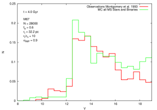
Figure 22: Comparison of the surface density profile and luminosity function for the Monte Carlo model for $\alpha_{IMF}=0.9$ and observations. The initial model parameters are described in the figures. The observational data is described in the text

The comparison between the luminosity functions from the Monte Carlo models and observations is given in the same figures as for the surface density profiles. The luminosity functions are in reasonable agreement with observations, except that the modelled luminosity function has an excess for $V>16$ mag, in comparison with observations. Of course there are also noticeable differences for the high-luminosity end connected with the relative lack of blue stragglers in the Monte Carlo models. It could be argued that the excess of low-luminosity stars cannot be explained by supposing that not all low-mass stars are observed, because the observational field of M67 is high-latitude, not heavily contaminated and sparse, and so all stars with $V\sim 18$ mag should be observed. On the other hand the authors themselves (Montgomery, Marschall & Janes, 1993) declared that the determination of the luminosity function “is a difficult procedure because of the presence of background stars”. Their background correction has been applied in the observational data shown in these figures, and they did it in the following way. The background was estimated by counting stars in an area of the colour-magnitude diagram just blue of the main sequence, and equal in area to the assumed boundaries of the main sequence. But photometric errors in the colours rise abruptly by $V=15$, and the resulting spread in the main sequence is very evident below $V=18$. If the result is that main sequence stars spread into the area in which field stars are counted, then the derived (observed) luminosity function will be too small.

Because of the difficulty in quantifying this effect, we should consider whether there are dynamical processes, omitted from the models, which could also account for the mismatch at the faint end of the luminosity function. The difference in the luminosity functions for $V>16$ mag suggests some mechanism by which the open cluster M67 very efficiently removed a substantial fraction of low mass stars ($M<0.7M_{\odot}$) during its evolution. There are two possibilities:

1. - removal of residual gas during the first few million years in a cluster with primordial mass segregation. The resulting expansion would lead to preferential removal of low mass stars.

2. - interactions with the galactic disk and bulge can produce tidal shocks which in turn again preferentially removes low mass stars (Spitzer, 1987). These effects would, of course, alter the entire history of mass-loss in the models, and require more massive initial models.

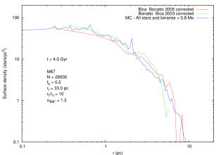
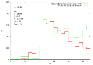
Figure 23: Comparison of the surface density profile and luminosity function for the Monte Carlo model for $\alpha_{IMF}=1.3$ and observations. The initial model parameters are described in the figures. The observational data is described in the text

Finally, we checked the influence of statistical fluctuations, which are intrinsic to the Monte Carlo method, on the determination of the initial cluster parameters which we have inferred from the comparison with observations. To assess the scale of this effect, the same model was repeated with different statistical realisations of the initial model, (i.e. different initial seeds (iseed) for the sequence of random numbers). Typical results are presented in Figs. 21 (Model III) and 24 (Model IV). It is clear that the use of different realisations of the initial model has a large impact on the observational properties of the cluster at time 4 Gyr. The good agreement for the surface density profile within the half-mass radius of the cluster is totally destroyed: the new model (iseed = 20) has a much higher central surface density, by factor of about 3. Also the luminosity function for model IV shows poorer agreement with the observations than model III: there are many more low-mass main sequence stars than in model III. As can be seen in the Tab. 6 the model with iseed = 20 is less advanced in its dynamical evolution. It has larger total mass and half-mass radius, and a smaller binary fraction. As can be seen in Fig. 24, at time 4.5 Gyr the model gives similar results to model III. Just because of the different statistical realisation of the initial conditions, model IV has smaller average mass than model III, and consequently smaller mass loss due to stellar evolution and a correspondingly smaller cluster expansion. The difference between the average masses is only about 4%, but it seems that this is enough to change the rate of cluster evolution substantially. This conclusion is supported by Hurley’s findings (Hurley, 2007) that the incidental formation of a massive binary can totally change the observational properties of the cluster.

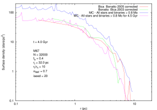
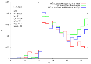
Figure 24: Comparison of the surface density profile and luminosity function for the Monte Carlo model for $\alpha_{IMF}=0.7$ and observations for different initial realisation of the models, iseed = 20. The initial model parameters are described in the figures. The observational data is described in the text

4 Discussion and Conclusions

In this paper we have presented an advanced Monte Carlo code for the evolution of rich star clusters, including most aspects of dynamical interactions involving binary and single stars, and the internal evolution of single and binary stars. It was shown that the free parameters of the Monte Carlo code can be successfully calibrated against results of small $N$-body simulations and simulations of the old open cluster M67.

Sec.3 described our best models of M67. The results show that an equally good fit to the observational data can be achieved by models which differ substantially in some initial parameters, such as the slope of the IMF. By contrast it seems that the other parameters are better constrained, at least within the ensemble of models which we studied. Actually, none of the models can successfully fit all the observational properties of M67 that we have studied, but we have argued that the remaining mismatches can be understood in terms of known characteristics of the Monte Carlo method, or the observational problem of subtracting the background. These difficulties are especially pronounced at the bright and faint ends of the luminosity function. The most satisfactory models are characterised by the following initial parameters: $N$ about 30000, $r_{t}$ about 33 pc, $f_{b}$ about 50% and $r_{t}/r_{h}$ about 10. The word “about” is used deliberately, because of the large effect of statistical fluctuations in such small systems. It is worth noting that a satisfactory fit can be achieved for a large range of values of the power-law index of the IMF for low mass stars, though it seems that values of $\alpha_{IMF}$ in the range 0.5 – 0.7 give slightly better agreement with observations.

Finally, these Monte Carlo simulations clearly show the strong influence of statistical fluctuations on the observational properties of a cluster. In consequence it seems that recovery of the initial cluster parameters from a comparison between numerical models and observations may be very difficult or even impossible, particularly for models with low or moderate $N$. More observational data is needed to constrain the models better, but the data on such properties as the number of particular kinds of binaries, pulsars or blue stragglers seem to provide only very weak constraints.

Despite these successes in fitting $N$-body models and the open cluster M67, the code has some known shortcomings, which we summarise here.

1. Cross sections: it has become apparent (Fregeau & Rasio, 2007) that the use of cross sections can lead to some systematic errors in the evolution of core parameters and other quantities. Within the context of the Monte Carlo code we are working on, it is known how to replace these by explicit numerical calculation of the interactions (Giersz & Spurzem, 2003), and this will be our next improvement. One side effect of the current absence of explicit interactions is that we do not yet model collisions which occur during them; therefore one channel for the formation of blue stragglers is missing from these simulations.

2. Higher-order multiples: It is widely argued that primordial triples and higher multiples should be incorporated into simulations along with primordial binaries. In any case, hierarchical triples form abundantly in binary-binary interactions (Mikkola, 1984). Such higher-order multiples are ignored in the present Monte-Carlo code, as cross sections for interactions with other objects have not yet been devised. Hierarchical triples and higher-order multiples can be introduced as new species when explicit calculation of interactions has been incorporated.

3. Escape: the Monte Carlo code described here incorporates a tidal cutoff, and a simple modification based on the theory devised by Baumgardt (2001). Other treatments are possible and worth trying.

4. Rotation: the Monte Carlo code is based on spherical symmetry, and would require rather fundamental and very difficult reconstruction in order to cope with cluster rotation. As was pointed out by Kim, Lee & Spurzem (2004) the rotation only somewhat accelerates the rate of core collapse.

5. Static tide: the effect of tidal shocks have been extensively studied (e.g. Kundic & Ostriker (1995)) and it would be possible to add the effects as another process altering the energies and angular momenta of the stars in the simulations. The addition of tidal shocks will be more important when modelling Galactic globular clusters than open clusters, which usually are confined inside the Galactic disk.

Despite these limitations, some of which are difficult to cure, the Monte Carlo model presented in this paper shows its potential power in simulations of star clusters, from open clusters to rich globular clusters. Monte Carlo models are feasible in a reasonable time (a week or so) for globular clusters, which are too large for direct $N$-body models, and future papers in this series will present results on M4 and several other globular clusters. The data provided by Monte Carlo simulations are as detailed as those provided by an $N$-body code. No available simulation methods, except Monte Carlo and $N$-body methods, can really provide that kind of comprehensive information. Even when $N$-body simulations eventually become possible, Monte Carlo models will remain as a quicker way of exploring the parameter space for the large scale $N$-body simulations.

References

- Anderson et al. (2006) Anderson, J., Bedin, L. R., Piotto, G., Yadav, R. S. & Bellini, A. 2006, A&A, 454, 1029
- Angeletti, Dolcetta & Giannone (1980) Angeletti, L., Dolcetta, R. & Giannone, P. 1980, Ap&SS, 69, 45
- Baumgardt (2001) Baumgardt, H. 2001, MNRAS, 325, 1323
- Bedin et al. (2001) Bedin, L. R., Anderson, J., King, I. R. & Piotto, G. 2001, ApJ, 560, L75
- Bedin, Piotto & King (2003) Bedin, L. R., Piotto, G. & King, I. R., & Anderson, J. 2003, AJ, 126, 247
- Behler et al. (2003) Behler, R. H., Murphy, B. W., Cohn, H. N. & Lugger, P. M. 2003, Bulletin of the American Astronomical Society, 35, 1289
- Bica & Bonatto (2005) Bica, E. & Bonatto, C. 2005, A&A, 431, 943
- Bonatto & Bica (2003) Bonatto, C. & Bica, E. 2003, A&A, 405, 525
- Casertano & Hut (1985) Casertano, S. & Hut. P. 1985, ApJ, 298, 80
- Chernoff & Weinberg (1990) Chernoff, D. F. & Weinberg, M. D. 1990, ApJ, 351, 121
- Drukier (1992) Drukier, G. A. 1992, Ph.D. Thesis,
- Drukier (1993) Drukier, G. A. 1993, MNRAS, 265, 773
- Dull et al. (1994) Dull, J. D., Cohn, H. N., Lugger, P. M., Slavin, S. D. & Murphy, B. W. 1994, Bulletin of the American Astronomical Society, 26, 1487
- Dull et al. (1997) Dull, J. D. et al. 1997, ApJ, 481, 267
- Fregeau & Rasio (2007) Fregeau, J. & Rasio, F. 2007, ApJ, 658, 1047
- Giersz (1998) Giersz, M. 1998, MNRAS, 298, 1239
- Giersz (2001) Giersz, M. 2001, MNRAS, 324, 218
- Giersz (2006) Giersz, M. 2006, MNRAS, 371, 484
- Giersz & Heggie (1994) Giersz, M. & Heggie, D. C. 1994, MNRAS, 268, 257
- Giersz & Heggie (1996) Giersz, M. & Heggie, D. C. 1996, MNRAS, 279, 1037
- Giersz & Heggie (2003) Giersz, M. & Heggie, D. C. 2003, MNRAS, 339, 486
- Giersz & Spurzem (2003) Giersz, M. & Spurzem, R. 2003, MNRAS, 343, 781
- Grabhorn et al. (1992) Grabhorn, R. P., Cohn, H. N., Lugger, P. M. & Murphy, B. W. 1992, ApJ, 392, 86
- Grindlay et al. (2001) Grindlay, J. E., Heinke, C., Edmonds, P. D. & Murray, S. S. 2001, Science, 292, 2290
- Heggie, Portegies Zwart & Hurley (2006) Heggie, D. C., Portegies Zwart, S. & Hurley, J. 2006, New Astronomy, 12, 20
- Hénon (1971) Hénon, M. H. 1971, Ap&SS, 14, 151
- Hénon (1975) Hénon, M. 1975, IAU Symp. 69: Dynamics of Stellar Systems, 69, 133
- Howell, Guhathakurta & Tan (2000) Howell, J. H., Guhathakurta, P. & Tan, A. 2000, AJ, 119, 1259
- Hurley (2007) Hurley, J. R. 2007, MNRAS, 379, 93
- Hurley, Pols & Tout (2000) Hurley, J. R., Pols, O. R. & Tout, C. A. 2000, MNRAS, 315, 543
- Hurley et al. (2005) Hurley, J. R., Pols, O. R., Aarseth, S. J. & Tout, C. A. 2005, MNRAS, 363, 293
- Hurley, Tout & Pols (2002) Hurley, J. R., Tout, C. A. & Pols, O. R. 2002, MNRAS, 329, 897
- Hut (2003) Hut, P. 2003, in Astrophysical Supercomputing Using Particle Simulations, IAU Symposium 208, ed.: P. Hut and J. Makino (San Francisco: the Astronomical Society of the Pacific), pp. 331-342.
- Joshi, Rasio & Portegies Zwart (2000) Joshi, K. J., Rasio, F. A. & Portegies Zwart, S. 2000, ApJ, 540, 969
- Kafka et al. (2004) Kafka, S., Gibbs, D. G., Henden, A. A. & Honeycutt, R. K. 2004, AJ, 127, 1622
- Kaliari et al. (2003) Kaliari, J. S., Fahlman, G. G., Richer, H. B. & Ventura, P. 2003, AJ, 126, 1402
- Kim, Lee & Spurzem (2004) Kim, E., Lee H. M. & Spurzem, R. 2004, MNRAS, 351, 220
- Kroupa (2007) Kroupa, P. 2007, arXiv:astro-ph/0703124
- Kroupa, Gilmore & Tout (1991) Kroupa, P., Gilmore, G. & Tout, C. A. 1991, MNRAS, 251, 293
- Kroupa, Tout & Gilmore (1993) Kroupa, P., Tout, C. A. & Gilmore, G. 1993, MNRAS, 262, 545
- Kundic & Ostriker (1995) Kundic, T. & Ostriker. J. P. 1995, ApJ, 438, 702
- Meylan & Heggie (1997) Meylan, G. & Heggie, D. C. 1997, A&A Rev., 8, 1
- Murphy et al. (1994) Murphy, B. W., Cohn, H. N., Lugger, P. M. & Dull, J. D. 1994, Bulletin of the American Astronomical Society, 26, 1487
- Murphy et al. (1997) Murphy, B. W., Cohn, H. N., Lugger, P. M. & Drukier, G. A. 1997, Bulletin of the American Astronomical Society, 29, 1338
- Murphy et al. (2003) Murphy, B. W., Cohn, H. N., Lugger, P. M. & Drukier, G. A. 2003, Bulletin of the American Astronomical Society, 35, 735
- Murphy et al. (1998) Murphy, B. W., Moore, C. A., Trotter, T. E., Cohn, H. N. & Lugger, P. M. 1998, Bulletin of the American Astronomical Society, 30, 1335
- Mikkola (1984) Mikkola, S. 1984, MNRAS, 207, 115
- Montgomery, Marschall & Janes (1993) Montgomery, K. A., Marschall, L. A. & Janes, K. A. 1993, AJ, 106, 181
- Piotto et al. (2002) Piotto, G. et al. 2003, A&A, 391, 945
- Portegies Zwart & Verbunt (1996) Portegies Zwart, S. F. & Verbunt, F. 1996, A&A, 309, 179
- Richer et al. (2004) Richer, H. B. et al. 2004, AJ, 127, 2771
- Sills et al. (2003) Sills, A. et al. 2003, New Astronomy, 8, 605
- Spitzer (1987) Spritzer, L. 1987, Princeton, NJ, Princeton University Press
- Stodołkiewicz (1986) Stodołkiewicz, J. S. 1986, Acta Astronomica, 36, 19