Observer dependence of the quasi-local energy and momentum in Schwarzschild space-time

Abstract

The observer dependence of the quasi-local energy (QLE) and momentum in the Schwarzschild geometry is illustrated. Using the Brown-York prescription, the QLE for families of non-geodesic and geodesic observers penetrating the event horizon is obtained. An explicit shell-building process is presented and the binding energy is computed in terms of the QLE measured by a static observer field at a radius outside the horizon radius. The QLE for a radially geodesic observer field freely-falling from infinity is shown to vanish. Finally, a simple relation for the dynamics of the quasi-local momentum density for a geodesic observer field is noted.

I Introduction

There has been rising interest in studying the quasi-local energy (QLE) inside the event horizon of the Schwarzschild geometry Lundgren:2006fu ; Blau:2007wj . However, the absence of physical, static observers on the interior, as exist on the exterior, has prevented a simple passage of QLE across the horizon. The alternative is then to identify families of non-static, non-geodesic and geodesic observers that can actually penetrate the horizon smoothly and measure the QLE. This is the main focus of the present work. It is hoped that this note can bring to the ongoing discussion a somewhat different perspective.

It is well-known that the quasi-local energy is observer dependent Brown:1992br . Take the Brown-York QLE for example, a family of prescribed observers – interchangeably referred to as an observer field – on a closed, orientable, space-like 2-surface, $S$, as embedded in a space-like hypersurface $\Sigma$ in the space-time manifold $M$, set up their frame fields and evaluate the trace of the mean curvature of $S$ as embedded in $\Sigma$ at their respective locations. After averaging over $S$ and calibrating against the Minkowski space reference, the ultimate quantity is the measured QLE associated with $S$. Among a sea of available observers in a space-time, the most physically meaningful ones are the observer fields that are static and those that are geodesic. In the Schwarzschild space-time, no static observer fields can enter the event horizon; on the other hand, there do exist geodesic observer fields that can cross the event horizon. Hence, to use one observer field as a probe to measure the QLE in the Schwarzschild space-time, the best candidates would be a non-static, observer field that penetrates the horizon or a geodesic observer field.

The Brown-York QLE measured by the above two kinds of observer fields in the Schwarzschild geometry are examined in this article. Generalizations to other spherically symmetric space-times should be straightforward. A simple observation regarding the dynamics of the relative quasi-local momentum density in a geodesic observer field is also presented.

A note about the Liu-Yau QLE Liu:2003 in the Schwarzschild space-time is recorded here as a comparison. Since the construction of the physical part of the Liu-Yau QLE employs a co-dimension 2 embedding of $S$, it is independent, in the exterior of the horizon, of the choice of observer field. However, the Liu-Yau QLE becomes invalid in the interior since the mean curvature vector of $S$ in $M$ becomes time-like, violating one of its defining hypotheses.

The structure of this article is as follows. An expeditious review of the fundamentals of the Schwarzschild and Kruskal space-times is given in Sec. II. Static and non-static, non-geodesic observer fields are used in the study in Sec. III, whereas the case of a geodesic observer field is presented in Sec. IV. Physical interpretations of the results are summarized in Sec. V.

II A Review of Definitions

Collected here are some necessary definitions and facts that are frequently referred to throughout the article. Hence, notations and terminology are unified in a consistent fashion, at the outset. It should be duly acknowledged that equivalent co-ordinate systems, such as those due to Novikov, Painleve, and Eddington-Finklestein, may as well be adopted for the problem at hand. The ones employed in the present work are an impartial choice at the service of highlighting the geometric nature. Details can be found in Ref. SachsWu1977 , for example.

The Schwarzschild space-time $({\cal M},g,D)$ consists of two connected components ${\cal M}=N\cup B$, namely its exterior $N=P_{\rm I}\times_{\rm r}S^{2}$, where $P_{\rm I}=p^{-1}({\mathds{R}}^{1}\times(2{\rm M},+\infty))$, and its interior $B=P_{\rm II}\times_{\rm r}S^{2}$, where $P_{\rm II}=p^{-1}({\mathds{R}}^{1}\times(0,2{\rm M}))$, each, in the form of warped product, equipped, in the Schwarzschild spherical co-ordinate system $x=p\times s$, where $p=(t,r)$ on $P=P_{\rm I}\cup P_{\rm II}$ and $s=(\vartheta,\varphi)$ on $S^{2}$, with the metric $g=g_{\rm P}+r^{2}g_{\rm S}$, where $g_{\rm P}=-h(r)dt\otimes dt+{dr\otimes dr}/{h(r)}$, $h(r)=1-{2{\rm M}}/{r}$ ($M>0$), and $g_{\rm S}$ the standard metric on $S^{2}$. $D$ is the Levi-Civita connection of $g$.

It is also quoted here, for notational purposes, the very basics of the Kruskal space-time that are referred to in the following section. The Kruskal plane $Q$ is obtained by joining the two connected components $P_{\rm I}$ and $P_{\rm II}$ via a diffeomorphism $f:{\mathds{R}}^{+}\longrightarrow(-{2{\rm M}}/{e},+\infty)$ by $f(r)=(r-2{\rm M})e^{\frac{r}{2{\rm M}}-1}$, ${\rm M}>0$. In terms of the Kruskal null co-ordinate functions $k=(u,v)\in{\mathfrak{F}}({\mathds{R}}^{2},{\mathds{R}})$ on the $u-v$ plane, $Q=k^{-1}\Big{(}\{(u,v)\in{\mathds{R}}^{2}:uv>-{2{\rm M}}/{e}\}\Big{)}$. The Schwarzschild co-ordinate functions $p=(t,r)$ on $Q$ become $t(u,v)=2{\rm M}{\rm log}|{v}/{u}|$ on $Q-Q_{\rm H}$, where $Q_{\rm H}=k^{-1}(\{(u,v)\in k(Q):uv=0\})$, and $r(u,v)=f^{-1}(uv)$ on $Q$. Thus, the metric on $Q$ reads $g_{\rm Q}=F(r)(du\otimes dv+dv\otimes du)$, where $F(r)=\frac{8{\rm M}^{2}}{r}e^{1-\frac{r}{2{\rm M}}}$, $\forall r\in{\mathds{R}}^{+}$. The Kruskal space-time, which is inextendible and incomplete, is the warped product $K=Q\times_{\rm r}S^{2}$, equipped with the metric $g_{\rm K}=g_{\rm Q}+r^{2}g_{\rm S}$. The four connected components, $\{Q_{j}\}_{j={\rm I}}^{j={\rm IV}}$, of $Q-Q_{\rm H}$ consisting of four open quadrants in the Kruskal plane, when lifted to $K$, yield $K_{\rm III}\approx K_{\rm I}\approx N$ and $K_{\rm IV}\approx K_{\rm II}\approx B$, by virtue of the isometries that preserve the Schwarzschild functions $p$. It is therefore sufficient to consider half of the Kruskal space-time.

The notions of a family of observers and an observer field (aka a reference frame) are used interchangeably throughout, the definition of which is adopted from Ref. SachsWu1977 . Namely, an observer field $Q$ on a space-time ${\cal M}$ is a vector field each of whose integral curves is an observer, where an observer is a future-directed time-like curve $\gamma:\mathscr{E}\longrightarrow{\cal M}$ with unit speed.

III Measurement by non-geodesic observers

III.1 Static observer field

The Schwarzschild exterior $N$, oriented by a nowhere-vanishing volume form $\Omega$ and time-oriented by defining the time-like Killing vector field $\frac{\partial}{\partial t}$ to be future-directed, is static with respect to the Schwarzschild observer field $U=\frac{1}{\sqrt{h(r)}}\frac{\partial}{\partial t}$, where $h(r)\in(0,1)$ on $N$. Since $D_{U}U=\frac{{\rm M}}{r^{2}}\frac{\partial}{\partial r}$, $U$ is not geodesic. The Schwarzschild interior $B$, however, is not static with respect to any observer field. Hence, Schwarzschild observers, i.e., integral curves of $U$, exist only in $N$, as $U$ becomes space-like in $B$. What inhabits $B$, nonetheless, is a geodesic observer field $V=-\sqrt{-h(r)}\frac{\partial}{\partial r}$, which is proper-time synchronizable since the dual frame field is $\theta^{\rm V}=-dg$, where $g(r)=\int\limits_{r^{\prime}=r_{0}}^{r}\frac{dr^{\prime}}{\sqrt{-h(r^{\prime})}}$, for some $r_{0}\in{\mathds{R}}^{+}$.

The Brown-York QLE measured by the Schwarzschild observer field in $N$ is

$${\rm QLE}(r)=r[1-\sqrt{h(r)}].$$ (1)

It is related to the ADM energy ${\rm M}$ for a spherically symmetric matter distribution via Brown:1992br

$${\rm M}={\rm QLE}(r_{*})-\frac{{\rm QLE}^{2}(r_{*})}{2r_{*}},$$ (2)

where $r_{*}$ is the outer boundary of the distribution and ${\rm M}=m(r_{*})$. The negative energy term on the right-hand side is interpreted in Brown:1992br as the negative energy outside of the matter distribution that equals the Newtonian gravitational binding energy associated with building a spherically symmetric shell with matter-energy ${\rm QLE}$ and radius $r_{*}$. In what follows, a hypothetical quasi-equilibrium procedure of constructing a spherically symmetric shell of gravitational mass ${\rm M}$ is described. The negative of the work done by the static Schwarzschild observer field $U$ to build up such a shell is explicitly computed.

Initially, no mass distribution is present. The Schwarzschild observer field $U$ starts moving from infinity, in a precisely spherically symmetric manner, a dust-shell of gravitational mass $dm$ and of zero thickness to a fixed radius $r_{*}$ which is outside of the horizon radius. It is assumed that each step is within quasi-equilibrium in the sense that staticity of the space-time is not sabotaged. It appears also legitimate to require that $dm$ be small enough so that the influence of the dust shell on $N$ is negligible. Moreover, the accumulation of mass on the shell at radius $r_{*}$ does not incur an expansion in its radius. Hence, no mechanism is provided to sustain the shell at rest; eventually, the shell of total gravitational mass ${\rm M}$ serves as an equivalent description of a spherically symmetric relativistic star of total gravitational mass ${\rm M}$ and radius $r_{*}$ seen from outside. More precisely, each of the instantaneous observers at $z\in N$ with co-ordinates $x(z)=(t,r,\vartheta,\varphi)$, carrying in $T_{z}N$ an orthonormal frame $X=\{U,X_{2},X_{3},X_{4}\}$, is referred to as $(z,X)$. The comoving dust-shell flow is modeled by its energy stress SachsWu1977 $T=\sigma\theta^{\rm U}\otimes\theta^{\rm U}$, where the gravitational mass surface density $\sigma$ measured by $(z,X)$ takes the form, in the Schwarzschild spherical co-ordinate system $x$, $\sigma\circ x=\frac{dm}{4\pi r^{2}\sqrt{h(r,m)}}\delta(x^{1}-r)$ and $\theta^{\rm U}$ is the dual of $U$. Here, a more explicit notation $h(r,m)=1-\frac{2m}{r}$ is employed purely to emphasize the dependence on the mass parameter. The use of the Dirac measure in the co-ordinate representation of $\sigma$ is but to indicate that ${\rm supp}(\sigma\circ x)$ is the shell of radius $r$ with zero thickness.

Before carrying out the computations, it seems worthwhile clarifying here the meaning of “work”. The absence of a globally defined inertial reference frame in $N$ prohibits any definition of work in the Newtonian fashion. However, the comoving feature of the dust-shell described above facilitates the evaluation of the work done by the observer field $U$ in the general relativistic context. An intuitive physical picture of the hypothetical shell-building process resembles very much a bucket brigade, where, by virtue of the spherical symmetry, the observer field $U$ is regarded as a continuum of radially lined up observers each exercising a certain amount of work moving a bit of the gravitational mass of the shell infinitesimally at their respective location. The total work, being a scalar, is registered as the sum of the infinitesimal work from each step. Precise calculations are as follows.

Suppose there exists already a spherical shell of gravitational mass $m$ at radius $r_{*}$. In the instantaneous inertial frame of each $(z,X)$, with $x^{1}(z)=r>r_{*}$, the measured infinitesimal gravitational mass density $\sigma=T(U,U)$ gets moved at the acceleration $A=D_{U}U=\frac{m}{r^{2}\sqrt{h(r,m)}}X_{2}$ by an infinitesimal “proper” radial distance $-\theta^{2}=-\frac{dr}{\sqrt{h(r,m)}}$. The infinitesimal work done in each such step amounts, in the continuous limit, to the total work done by the observer field $U$ throughout the entire moving process:

$$W_{U}=\int\limits_{0}^{{\rm M}}\int\limits_{+\infty}^{r_{*}}\int\limits_{S^{2}}(\sigma\circ x)|_{x^{1}=r}g(A,X_{2})\Omega_{S^{2}}(-\theta^{2})$$ (3)

$$\qquad\qquad=-{\rm M}+r_{*}(1-\sqrt{h(r_{*})}),$$

where $\Omega_{S^{2}}$ is the standard volume form on $S^{2}$ and $h(r_{*})=1-\frac{2{\rm M}}{r_{*}}\in(0,1)$. Written in a more suggestive form, the above relation, ${\rm M}={\rm QLE}(r_{*})+(-W_{\rm U})$, is precisely Eq. (2).

Recall the known inequality Bizon:1990nk on the total gravitational energy of a spherically symmetric distribution of matter which is instantaneously at rest: ${\rm M}\leq{\rm M}_{\rm p}-E_{\rm B}$, where ${\rm M}$ and ${\rm M}_{\rm p}$ are the total gravitational and the proper mass of the distribution, respectively, and $E_{\rm B}$ is the binding energy. The equality is achieved if and only if the general relativistic configuration possesses the least binding energy, i.e., a spherically symmetric shell as in the Newtonian limit. When ${\rm QLE}(r_{*})$ is understood to be the proper energy within the radius $r_{*}$ as in Brown:1992br , $W_{\rm U}$ gives the least binding energy required for the spherically symmetric shell configuration.

The geometry of the exterior of a spherically symmetric relativistic star is known to be modeled by the Schwarzschild exterior $(N,g)$, provided that the horizon is frozen inside the surface of the star. As another example, the QLE of a spherically symmetric star is easily computed. For a mass density $\rho(r)$, the gravitational mass contained within a radius $r$ is $m(r)=4\pi\int dr\,r^{2}\rho(r)$. Eq. (1) indicates that the slope of the QLE is discontinuous across the surface of the star. Furthermore, based on the positivity of the mass density, the QLE is a maximum at the surface of the star. Specifically, consider the case of a constant density star of radius $r_{*}$ and gravitational mass ${\rm M}\in(0,\frac{4}{9}r_{*})$, with Schwarzschild radius $r_{S}=2{\rm M}<r_{*}$. The QLE is

$${\rm QLE} = 2{\rm M}\frac{r}{r_{S}}[1-\sqrt{h(r)}]$$ (4)

$$h(r) = 1-\frac{r_{S}}{r}\left(\left(\frac{r}{r_{*}}\right)^{3}\Theta(r_{*}-r)-\Theta(r-r_{*})\right)$$ (5)

where $\Theta$ is the Heaviside function. The QLE grows inside the star from the center to the surface, whereupon it decays to ${\rm M}$ at infinity (see Figure 1). The left (resp. right) radial derivative of the QLE at $r_{*}$ tends to $+\infty$ (resp. $-\infty$) as $r_{\rm S}$ approaches $r_{*}$.

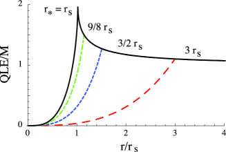
Figure 1: The BY QLE for stationary, non-geodesic observers outside a constant desity star of mass $M$ and radius $r_{*}$ is shown. Four cases are shown corresponding to $r_{*}/r_{S}=1$ (unstable, solid), and $r_{*}/r_{S}=9/8,\,3/2,\,3$ (long-short-dashed, short-dashed, long-dashed lines) where $r_{S}=2{\rm M}$ is the Schwarzschild radius of the star. In all cases, the slope of the QLE is discontinuous at the surface of the star.

III.2 Non-static observer field

It is natural to seek the QLE inside the horizon, in $B$ as well. The investigation has been carried out recently in Ref. Lundgren:2006fu , wherein an attempt has been made to continue the family of static, non-geodesic Schwarzschild observers from $N$ into $B$. The result is that the unit normal of $S^{2}$ as embedded in the space-like hypersurface $\Sigma$ is chosen to be time-like in $B$ (c.f. Eq.(16) in Lundgren:2006fu ), thereby forcing the observer field to be space-like in $B$. This unphysical choice for the observers seems incompatible with the construction of the Brown-York QLE. The result in Lundgren:2006fu , for Schwarzschild space-time, is invoked in Blau:2007wj to establish the relationship between the Brown-York QLE measured by the radial geodesic observers in $N\cup B$ and the effective potential of the radial time-like geodesics. However, the observers used in Lundgren:2006fu are not geodesic and are valid in $N$ only, which makes the analysis in Blau:2007wj less justified. If instead the geodesic observer field $V$ is employed in $B$, then the resulting QLE is simply ${\rm QLE}=r$, which matches Eq. (1) at the black hole horizon. Similar calculations in more general settings have been carried out in Booth:1998eh , where the “non-orthogonal” boundaries are taken into account. The non-orthogonality comes about by flowing the 2-dimensional closed orientable space-like surface $S$ along an observer field $T$ that differs from the unit time-like vector field $U$ that is orthogonal to the 3-dimensional space-like hypersurface into which $S$ is isometrically embedded. Such scenarios are of physical interest when the so called “boosted” observer fields are considered. As a consequence, a generalized reference embedding scheme has to be devised to adapt the foliation of $S$ along the flow of $T$. In particular, for the Schwarzschild space-time $N\cup B$, a natural choice of $U$ in $N$ is the Schwarzschild static observer field, with respect to which the observer field $T$ can be put in the form such as Eq.(30) in Ref. Booth:1998eh . The different time orientation in $B$, however, spoils the foliation by the privileged static observer field and thus invalidates the choice of $T$ for $N$. Additional comparison with the results in Ref. Booth:1998eh for the geodesic observer field in Schwarzschild geometry is given in Sec. IV. In addition, so far as measurements are concerned, it is always possible to associate to the observer field 2-dimensional closed orientable and space-like surfaces in the orthogonal fashion as shown in what follows.

The crux of the matter is an observer field that can penetrate the Schwarzschild horizon $r_{S}=2{\rm M}$. Such observer fields do exist. It is perhaps more convenient to use the Kruskal space-time $K$. Note that the radius function $r$ is well defined on all of $K$, whereas the time function $t$ is defined only on $K-H$, where $H$ is the lift of $Q_{\rm H}$ and represents the event horizon. By construction, $Y=\frac{1}{4{\rm M}}(v\frac{\partial}{\partial v}-u\frac{\partial}{\partial u})$ is a Killing vector field on $K$ and equals $\frac{\partial}{\partial t}$ on $K-H$, but $\frac{\partial}{\partial t}$ can be uniquely extended as a Killing field over all of $K$. Hence, the Kruskal space-time can be time-oriented, in accord with the physical interpretations on $N$, by requiring that $\frac{\partial}{\partial t}$ be future-directed on $K_{\rm I}$.

Clearly, the observer field of interest here cannot be $Y$, which changes its chronological signature in $K_{\rm II}$. It is, however, chosen, among others, to be $X_{1}=\frac{1}{\sqrt{2F(r)}}(-\frac{\partial}{\partial u}+\frac{\partial}{\partial v})$, with its dual $\theta^{1}=\sqrt{\frac{F(r)}{2}}d\xi$, where $\xi=-u+v$. Hence, $X_{1}$ is synchronizable, i.e., there exists a unique space-like hypersurface $\Sigma$ of ${\cal M}$, the distribution on which is annihilated by $\theta^{1}$, and thus completely integrable. Furthermore, the co-ordinate function $\xi\circ\iota=\xi_{0}({\rm const.})$, where $\iota:\Sigma\hookrightarrow{\cal M}$. Given $X_{1}$, there exists $X_{2}=\frac{1}{\sqrt{2F(r)}}(\frac{\partial}{\partial u}+\frac{\partial}{\partial v})$, with its dual $\theta^{1}=\sqrt{\frac{F(r)}{2}}d\rho$, where $\rho=u+v$, such that $X_{2}$ is space-like and $\theta^{1}(X_{2})=0$. Consequently, $X_{2}\circ\iota=X_{2}$ and in $\Sigma$, there exists a unique space-like hypersurface $S$ of $\Sigma$, the distribution on which is annihilated by $\theta^{2}$ and thus completely integrable. Similarly, the co-ordinate function $\rho\circ\eta=\rho_{0}({\rm const.})$, where $\eta:S\hookrightarrow\Sigma$. Thus, on $S$, $\xi=\xi_{0}$ and $\rho=\rho_{0}$, and correspondingly, $t=t(\xi_{0},\rho_{0})={\rm const.}$ and $r=r(\xi_{0},\rho_{0})={\rm const.}$, which implies that $(\iota\circ\eta)^{\ast}g=r^{2}g_{\rm S}$. That is, $S=S^{2}$. To complete the frame field for the observer field, pick the usual orthonormal frame on $S^{2}$, namely, $X_{3}=\frac{1}{r}\frac{\partial}{\partial\vartheta}$ and $X_{4}=\frac{1}{r{\rm sin\vartheta}}\frac{\partial}{\partial\varphi}$, with their duals $\theta^{3}=rd\vartheta$ and $\theta^{4}=r{\rm sin\vartheta}d\varphi$, respectively.

The core of the calculation in Brown-York QLE is the mean curvature of $S^{2}$ as embedded in $\Sigma$. However, substantial simplifications are readily available in the current setting. Since $X_{2}\in\Gamma(\Sigma,T\Sigma)$, the induced connection ${\widetilde{D}}$ of $D$ on $\Sigma$ coincides with the Levi-Civita connection $D^{\Sigma}$ of $\Sigma$, thus, the second fundamental form of $S^{2}$ as embedded in $\Sigma$ with its normal $X_{2}$ is given by

$$\mathrm{I\!I}(X_{l},X_{l}) = -\iota^{\ast}g({\widetilde{D}}_{\eta_{\ast}X_{l}}X_{2}\circ\iota,\eta_{\ast}X_{l})$$ (6)

$$= -g(D_{\eta_{\ast}X_{l}}\iota_{\ast}(X_{2}\circ\iota),\eta_{\ast}X_{l})$$

$$= \theta^{2}(D_{\eta_{\ast}X_{l}}\eta_{\ast}X_{l}),$$

for $l=3,4$. Standard Cartan calculus shows that $\mathrm{I\!I}(\theta^{3},X_{3})=\mathrm{I\!I}(\theta^{4},X_{4})=\omega^{2}_{3}(\eta_{\ast}X_{3})=-\frac{\sqrt{2F(r)}}{8Mr}(u+v)$, where $\omega$ is the connection 1-form on $M$. Hence, the trace of the mean curvature is $k={\rm tr}\mathrm{I\!I}=-\frac{\sqrt{2F(r)}}{4{\rm M}r}(u+v)$. On the other hand, the flat-space reference embedding $\eta^{0}:S^{2}\hookrightarrow{\mathds{R}}^{3}$ yields $k^{0}={\rm tr}\mathrm{I\!I}^{0}=-\frac{2}{r}$. Therefore, the Brown-York QLE is given by

$${\rm QLE}(t,r) = \frac{1}{8\pi}\int\limits_{S^{2}}(k-k^{0})\Omega$$ (8)

$$= r\Big{[}1-\frac{\sqrt{2F(r)}}{8{\rm M}}(u+v)\Big{]}$$

$$= r\Big{[}1-\delta\sqrt{h(r)}{\rm cosh}(\frac{t}{4{\rm M}})\Big{]},$$

where $\Omega$ is the volume form of $S^{2}$ and $\delta=1$ on $K_{\rm I}$ (exterior) and $-1$ on $K_{\rm II}$ (interior).

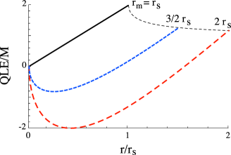
Figure 2: The Brown-York QLE for non-geodesic observers, $X_{1}$, outside a black hole of mass ${\rm M}$ is shown. Three cases are shown, corresponding to maximum radius given by $r_{\rm max}/r_{S}=1,3/2,2$ (solid, short-dashed, long-dashed lines). Note that QLE decreases smoothly as the observer crosses the horizon.

The QLE measured by the observers $X_{1}$ on $S^{2}$ depends on both Schwarzschild functions $t$ and $r$, subject to the conditions $\xi\circ\iota={\rm const}.$ and $\rho\circ\eta={\rm const}.$. This result differs from that measured by the Schwarzschild observers $U$ in $N$ because $X_{1}$ and $U$ produce different foliations of the space-time manifold. The key difference, though, is that $X_{1}$ is an observer field over all of $K$, while $U$ is defined on $N\approx K_{\rm I}$ only. The QLE is illustrated in Fig. 2. In contrast to the case of the static observer field, $D_{X_{1}}X_{1}=-\frac{1}{16{\rm M}}(u+v)(\frac{1}{r(u,v)}+\frac{1}{2{\rm M}})\sqrt{2F}X_{2}$, the work done by $X_{1}$ to build up the spherically symmetric shell of gravitating mass ${\rm M}$ and radius $r_{*}$ is negative for $r_{*}\in{\rm QLE}^{-1}({\mathds{R}}^{-})$.

IV Measurement by geodesic observers

A different type of observer field of physical interest is the geodesic observer field in $N\cup B$, which crosses the event horizon. The isometries of $S^{2}$ admit a system of the Schwarzschild spherical co-ordinates with respect to which each of the geodesic observers, $\gamma:{\mathscr{E}}\longrightarrow{\cal M}$, is initially equatorial, i.e., $\vartheta\circ\gamma\equiv\frac{\pi}{2}$, and thus, $X_{1}={\dot{\gamma}}=\frac{E}{h(r)}\frac{\partial}{\partial t}+\delta\sqrt{E^{2}-V(r)}\frac{\partial}{\partial r}+\frac{L}{r^{2}}\frac{\partial}{\partial\varphi}$, depending upon whether the geodesic is ingoing ($\delta=-1$) or outgoing ($\delta=+1$). Here the constants $L$, the angular momentum per unit mass of the observer, and $E$, the energy per unit mass at infinity, are related via the energy equation $E^{2}=(\frac{d}{d\tau}(r\circ\gamma))^{2}+V(r)$, with $V(r)=(1+\frac{L^{2}}{r^{2}})h(r)$ being the effective potential. Of course, $X_{1}$, as a unit vector, is not defined on the horizon $H$, in the Schwarzschild spherical co-ordinates, as usual; the energy equation, nonetheless, holds by continuity.

For simplicity, only radial geodesics ($L=0$) are considered, in which case two kinds of ordinary orbits are available: (1) the crash orbit ($E^{2}\in(0,1)$), where ingoing observers crash directly into the singularity at $r=0$ and outgoing observers shoot out to a turning point $r_{\rm max}$ ($E^{2}=h(r_{\rm max})$) and then back into crash; (2) the crash/escape orbit ($E^{2}\in[1,+\infty)$), where ingoing observers crash while outgoing observers escape to infinity. In $N\cup B$, the radial geodesic observer field $X_{1}=\frac{\partial}{\partial\xi}$ is proper time synchronizable since the dual frame $\theta^{1}=d\xi$, where $\xi=Et-\int\limits_{r^{\prime}=r_{0}}^{r}\delta\frac{\sqrt{E^{2}-h(r^{\prime})}}{h(r^{\prime})}dr^{\prime}$. The rest of the construction follows the same lines as in Sec. III. There exists a space-like $X_{2}=\frac{1}{\sqrt{E^{2}-h(r)}}\frac{\partial}{\partial\rho}$ chosen to be consistent with the positive orientation of $\Sigma$ as embedded in $M$. $X_{2}$ is synchronizable since $\theta^{2}=\sqrt{E^{2}-h(r)}d\rho$, where $\rho=-\delta t+\int\limits_{r^{\prime}=r_{0}}^{r}\frac{Edr^{\prime}}{h(r^{\prime})\sqrt{E^{2}-h(r^{\prime})}}$. Hence, there exists a co-dimension 1 embedding $\eta:S=S^{2}\hookrightarrow\Sigma$ such that $\rho\circ\eta=\rho_{0}({\rm const.})$. The mean curvature of $S^{2}$ as embedded in $\Sigma$ with the unit normal $X_{2}=X_{2}\circ\iota$ is given by $k={\rm tr}\mathrm{I\!I}=-2\frac{E}{r}$, where $r=r(\xi_{0},\rho_{0})$, with the reference part intact. Therefore, the Brown-York QLE measured by the geodesic observer field in $N\cup B$, for crashing orbits, is ${\rm QLE}(r)=r(1-E)$, where $r\in(0,r_{\rm max}]$. Note that $E(r)$ remains valid at $r=2{\rm M}$ by continuity.

In contrast to the analysis in Blau:2007wj , the QLE measured by the geodesic observer field does not seem to be related to the effective potential in a non-trivial fashion. It is, however, simply linear in the radius function $r$. At the turning point $r_{\rm max}$ for crash orbits, ${\rm QLE}(r_{\rm max})=\frac{2{\rm M}}{1+E}$. At the event horizon, ${\rm QLE}(r)$ remains valid by continuity, and ${\rm QLE}(r=2{\rm M})=2{\rm M}(1-E)$. A critical situation is when $E^{2}=1$ and each observer in this geodesic observer field starts at rest from infinity. In the course of freely falling towards the singularity, the QLE measured by this family of geodesic observers vanishes identically. Interestingly, when $E^{2}>1$, the QLE become negative. This result follows from the definition of the Brown-York QLE, whose sign is determined by that of the sectional curvature of the 3-dimensional space-like hypersurface $\Sigma$ into which the 2-dimensional consistently oriented, closed, space-like surface $S$ is isometrically embedded. For the geodesic observer field $X_{1}$, the sectional curvature of $\Sigma$ is $K(\Sigma)=\frac{1-E^{2}}{r^{2}}$, which is positive ($E^{2}\in(0,1)$), zero ($E^{2}=1$), or negative ($E^{2}\in(1,+\infty)$). When compared to the reference term evaluated in ${\mathds{R}}^{3}$, the Brown-York QLE becomes positive, zero, or negative, respectively. In Figure 3, different QLE measurements are plotted for illustrative purposes.

These results are different from those measured by the radially infalling observers with $E=1$ considered in Ref. Booth:1998eh . As explained in Sec. III, the discrepancy arises from the generalized embedding scheme (c.f. Eq.(40)) in Booth:1998eh , in accord with the non-orthogonal boundaries. Should an $S^{2}$ that is orthogonal to $T$ be used in Booth:1998eh , the same QLE as given here follows immediately.

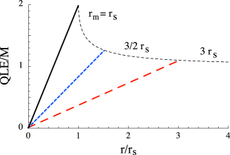
Figure 3: The Brown-York QLE for geodesic observers outside a black hole of mass $M$ is shown. Three cases are shown, corresponding to bound trajectories with energy per unit mass $E=\sqrt{h(r_{\rm max})}$ starting at a maximum radius given by $r_{\rm max}/r_{S}=1,3/2,3$ (solid, short-dashed, long-dashed lines). Note that QLE decreases smoothly as the observer crosses the horizon. In the case of an observer starting at $r_{\rm max}/r_{S}\to\infty$, the QLE is zero.

It is curious to note that a star with mass density $\rho\propto r^{-2}$, albeit unphysical due to the existence of a curvature singularity at the origin, gives rise to a well-behaved QLE. In view of Eq.(5) for observers $U$ in $N$, and observers $V$ in $B$, ${\rm QLE}=2{\rm M}\frac{r}{r_{S}}[1-\sqrt{h(r)}]$ with $h(r)=1-\frac{r_{S}}{r_{*}}\Theta(r_{*}-r)-\frac{r_{S}}{r}\Theta(r-r_{*})$. The non-geodesic, stationary observer QLE curves in the limiting case $r_{*}/r_{S}\to 1$ and $r_{*}/r_{S}=3/2,\,3$ coincide with the curves for geodesic observers shown in Figure 3.

The rest of this section is devoted to a discussion of the measurement of the quasi-local momentum by a family of geodesic observers. Similar analysis can be carried out, though more complicated, for non-geodesic observers, as well.

Consider an orthonormal frame field $\{X_{i}\}_{i=1}^{i=4}$, in which $X_{1}$ is time-like geodesic and (locally) synchronizable. $\forall p\in{\cal M}$, $T_{p}{\cal M}={\mathds{R}}X_{1}\oplus{\rm R}_{p}{\cal M}$, where ${\rm R}_{p}{\cal M}={\rm span}_{\mathds{R}}\{X_{i}\}_{i=2}^{i=4}$. The Brown-York quasi-local momentum density ${\mathscr{J}}\in R^{\ast}{\cal M}$ is defined by Brown:1992br ${\mathscr{J}}(Y_{p})=-\frac{1}{8\pi}\Big{(}\Theta\iota^{\ast}g(Y_{p},X_{2})-\mathrm{I\!I}^{X_{1}}(Y_{p},X_{2})\Big{)}$, $\forall(p,Y_{p})\in R^{\ast}{\cal M}$, where $\Theta={\rm div}X_{1}$ is the expansion of the (local) flow of $X_{1}$ and $\iota:\Sigma\hookrightarrow{\cal M}$ is the (local) embedding induced by $X_{1}$. When restricted to the 2-dimensional orientable closed space-like surface $S$ embedded in $\Sigma$, whenever $\Sigma$ is completely integrable, $\mathscr{J}$ is the quasi-local momentum surface density $j$, as originally given in Brown:1992br . It is clear from the definition that the reference term for the quasi-local momentum vanishes identically when the flat-space reference is employed. Hence, only the physical part is considered in what follows.

Given a one-parameter family of time-like geodesics $x:{\mathscr{E}}\times(-\delta,+\delta)\longrightarrow{\cal M}$ around the base, $\gamma:{\mathscr{E}}\longrightarrow{\cal M}$ given by $\gamma u=x(u,0)$, where $\gamma_{\ast}\frac{d}{du}=X_{1}$, the Fermi-Walker connection SachsWu1977 coincides with the induced connection $\gamma^{\ast}D$ over $\gamma$. For economy of notation, there is no differentiation among various connections whenever the context is clear. Recall that a neighbor of the base is given by a Jacobi field, $J\in\Gamma({\mathscr{E}},R{\cal M})$, over $\gamma$, as those Jacobi fields that are tangent to $\gamma$ are of scant importance. It is then convenient to introduce the following natural decomposition: $J=J^{\bot}+J^{\top}$, where $J^{\bot}=\theta^{2}(J)$ and $J^{\top}=J-J^{\bot}$. Accordingly, the 3-relative quasi-local momentum density measured by a neighboring observer with respect to the base is ${\mathscr{J}}(J)={\mathscr{J}}(J^{\bot})+j(J^{\top})$. Thus, the Brown-York quasi-local momentum surface density $j(J^{\top})$ measured by the neighbor is the component that is tangent to $S$, the orthogonal complement being the normal stretch ${\mathscr{J}}(J^{\bot})$.

The relative quasi-local momentum density in the family of geodesic observers is obtained with the help of the Raychaudhuri equation for time-like geodesics. Further simplifications emerge as the space-time of interest is Ricci-flat. Since $X_{1}$ is (locally) synchronizable, hence irrotational SachsWu1977 , the Raychaudhuri equation becomes $\frac{d}{du}\Theta=-\frac{1}{3}\Theta^{2}-{\rm tr}(\sigma^{2})$, where $\sigma$ is the shear of $x$. Hence, $\frac{d}{du}{\mathscr{J}}(J)=-\frac{1}{8\pi}\Big{[}\Theta{\mathscr{J}}(J)-(\Theta^{2}+\mathrm{I\!I}^{X_{1}}\cdot\mathrm{I\!I}^{X_{1}})\iota^{\ast}g(J,X_{2})-g(R_{JX_{1}}X_{1},X_{2})\Big{]}$, where $\mathrm{I\!I}^{X_{1}}\cdot\mathrm{I\!I}^{X_{1}}=\sum\limits_{i=2}^{i=4}\sum\limits_{j=2}^{j=4}\mathrm{I\!I}^{X_{1}}(\theta^{i},\theta^{j})\mathrm{I\!I}^{X_{1}}(X_{i},X_{j})$. When restricted to $S$, it yields

$$8\pi\frac{d}{du}j(J^{\top})+\Theta j(J^{\top})=g(R_{J^{\top}X_{1}}X_{1},X_{2}),$$

where $g(R_{J^{\top}X_{1}}X_{1},X_{2})$ is the tidal force exerted on the neighbor tangent to $S$ in the $X_{2}$-direction.

It is hoped that the above analysis provides a slightly different perspective towards understanding the dynamics of the quasi-local momemtum measured by the family of geodesic observers.

V Summary and discussion

The measurements of the Brown-York QLE in Schwarzschild space-time by a non-static, non-geodesic observer field that penetrate the event horizon and by a geodesic observer field have been computed. It has been shown that due to a different space-time foliation induced by the observer field, the measurement of QLE by the non-static, non-geodesic observer field depends on both the radius function $r$ and the time function $t$. The QLE measured by a geodesic observer field is, however, linear in the radius function $r$, and can be positive, zero, or negative, depending upon the energy parameter of the geodesic observer field. These results differ significantly from the measurement by a static observer field in the Schwarzschild exterior $N$, which is previously known. On the other hand, the Liu-Yau QLE is independent of the choice of observer field in $N$ and coincides with the Brown-York QLE measured by the static observer field in $N$. However, the Liu-Yau QLE is not defined in Schwarzshild interior $B$ because the mean curvature vector of the co-dimension 2 isometric embedding of $S$ into $M$ becomes time-like.

To explore more about the physical nature of QLE, a hypothetical process of building a spherically symmetric massive shell by a static observer field was considered. The gravitational mass of the spherically symmetric shell is the QLE of the shell plus the negative gravitational potential energy associated with the work exercised to build the shell. The result holds for both the Brown-York and the Liu-Yau QLE since they coincide in $N$ for the static observer field. In addition, the QLE of a spherically symmetric star with constant density in the interior is also calculated. The QLE grows monotonically with respect to radial distance from the origin in the interior and drops off in the exterior towards the ADM mass ${\rm M}$ at infinity, with a cusp on the surface of the star. It seems to provide certain physical justification for QLE as a viable measure of energy.

For a geodesic observer field in the Schwarzshild geometry, a dynamic relation of the Brown-York quasi-local momentum density has been noted. It is valid for any Ricci-flat space-time. When a family of geodesic observers are assigned on $S$ to carry out physical measurements, this relation is expected to describe their relative dynamics. Generalization to more realistic Fermi-Walker observer fields is straightforward but more complicated.

- (1) A. P. Lundgren, B. S. Schmekel and J. W. York, Phys. Rev. D 75, 084026 (2007) [arXiv:gr-qc/0610088].
- (2) M. Blau and B. Rollier, arXiv:0708.0321 [gr-qc].
- (3) J. D. Brown and J. W. York, Phys. Rev. D 47, 1407 (1993).
- (4) C.-C. M. Liu and S.-T. Yau, Phys. Rev. Lett. 90, 231102 (2003).
- (5) R. K. Sachs and H. H. Wu, “General Relativity for Mathematicians” (Springer-Verlag, New York: 1977).
- (6) P. Bizon, E. Malec, and N. O’Murchadha, Class. Quant. Grav. 7, 1953 (1990).
- (7) I. S. Booth and R. B. Mann, Phys. Rev. D 59, 064021 (1999) [arxiv:gr-qc/9810009].