Cellular automata for the spreading of technologies in socio-economic systems

Abstract

We introduce an agent-based model for the spreading of technological developments in socio-economic systems where the technology is mainly used for the collaboration/interaction of agents. Agents use products of different technologies to collaborate with each other which induce costs proportional to the difference of technological levels. Additional costs arise when technologies of different providers are used. Agents can adopt technologies and providers of their interacting partners in order to reduce their costs leading to microscopic rearrangements of the system. Analytical calculations and computer simulations revealed that starting from a random configuration of different technological levels a complex time evolution emerges where the spreading of advanced technologies and the overall technological progress of the system are determined by the amount of advantages more advanced technologies provide, and by the structure of the social environment of agents. We show that agents tend to form clusters of identical technological level with a power law size distribution. When technological progress arises, the spreading of technologies in the system can be described by extreme order statistics.

, Gergely Kocsis, and János Farkas

1 Introduction

Recently, the application of statistical physics and of the theory of critical phenomena provided novel insight into the dynamics of socio-economic systems [1, 2, 3, 4, 5, 6, 7, 11]. Various types of models have been developed which capture important aspects of the emergence of communities [1], opinion spreading [2, 3, 4, 5, 6, 7] or the evolution of financial data [12]. The dynamics of innovation and the spreading of new technological achievements show also interesting analogies to complex physical systems [8, 9, 10, 11]. The process of innovation has recently been studied by introducing a technology space based on percolation theory [9]. In this model new inventions arise as a result of a random search in the technology space starting from the current best-practice frontier. The model could reproduce the interesting observation that innovations occur in clusters whose sizes are described by the Pareto distribution [9]. Another important aspect of technological development is the spreading of new technological achievements. In a socio-economic system different level technologies may coexist and compete as a result of which certain technologies proliferate while others disappear from the system. One of the key components of the spreading of successful technologies is the copying, i.e. members of the system adopt technologies used by other individuals according to certain decision mechanisms. Decision making is usually based on a cost-benefit balance so that a technology gets adopted by a large number of individuals if the upgrading provides enough benefits. The gradual adaptation of high level technologies leads to spreading of technologies and an overall technological progress of the socio-economic system.

In the present paper we consider a simple agent-based model of the spreading of technological achievements in socio-economic systems. Agents of the model may represent individuals or firms which use certain technologies to collaborate with each other. For simplicity, we assume that costs of the cooperation arise solely due to the incompatibility of technologies used by the agents which then have two origins: on the one hand, difference of technological levels incurs cost, the larger the difference is, the higher the cost gets. On the other hand, technologies used by agents may belong to different providers which induce additional costs. Agents interacting with their social neighborhood can decrease their cost by adopting technologies of their interacting partners. The local rejection-adaptation strategy of agents can lead to interesting changes of the system on the meso- and macro-level, namely, agents can form clusters with identical technological levels, which can also be accompanied by an overall technological progress of the system.

We analyze the time evolution of this model socio-economic system starting from a random configuration of technological levels and providers without considering the possibility of innovation. Based on analytic calculations and computer simulations we study how the adaptation of technologies of interacting partners leads to spreading of technological achievements. We characterize the microstructure of communities of agents, and the technological progress of the system on the macro level.

2 Model

Our model captures some relevant features of the spreading of technological developments when they are mostly used for the cooperation of individuals. In the model we represent the socio-economic system by a set of agents which posses products of different technological levels and use it to cooperate with each other. Thinking in terms of telecommunication technologies, agents are characterized by two variables: the technological level of the product an agent has (the technological level of the device the agent uses for communication) is described by a real variable $\tau$ such that a larger value of $\tau$ stands for more advanced technologies. New technologies developed by the producers reach the agents through providers. For simplicity, we assume that there are at most two providers active in the system and each agent belongs to one of them. The provider of agents is characterized by an integer variable $S$ which can take two different values $S=\{-1,1\}$.

The agents are assumed to cooperate with their social partners which is the easiest if the partners have products of the same technological level. Using technologies of different level can induce difficulties which may be realized by additional costs. It is reasonable to assume that the cost $C$ induced by the collaboration of agents $i$ and $j$ is a monotonous function of the difference of the technological levels $|\tau_{i}-\tau_{j}|$. For the purpose of the explicit mathematical analysis we consider the simplest functional form and cast the cost of cooperation into the following form

$$C(i\to j)=a|\tau_{i}-\tau_{j}|+\frac{1}{2}\Delta(1-S_{i}S_{j}).$$ (1)

The equation expresses that being at different technological levels (having different $\tau$ values) incurs cost, the higher the difference is in $\tau$ the higher the costs are, while being at the same technological level is cost-free. This crude assumption models a socio-economic system which favors the local communities to be at the same technological level. The value of the multiplication factor $a$ has to be chosen to capture the effect that in case of different technological levels it is favorable for agents to be on a higher technological level than their interacting partners. It follows that the value of $a$ should depend on the relative technological level of the agents with the condition

$$a=\left\{\begin{array}[]{lll}a_{1},&if&\tau_{i}>\tau_{j}\\ a_{2},&if&\tau_{i}<\tau_{j}\end{array}\ \ \ \ \ \ \mbox{where}\ \ \ \ \ a_{1}<a_{2}.\right.$$ (4)

The condition $a_{1}<a_{2}$ implies that being on a higher technological level, i.e. being more advanced than the surroundings $\tau_{i}>\tau_{j}$, can lower the costs compared to the opposite case. The second term of Eq. (1) takes into account that the cooperation of agents belonging to different providers implies additional expenses. We assume that this cost does not depend on the technological levels by setting $\Delta>0$ to a constant value. Note that $(1/2)(1-S_{i}S_{j})$ takes value 1 or 0 for agents of different and of the same providers, respectively, resulting in an additional cost $\Delta$ when agents of different providers collaborate. The arrow $\to$ in the argument of $C$ in Eq. (1) expresses that due to the condition Eq. (4) the cost function is not symmetric with respect to agents $i$ and $j$. Hence, $C(i\to j)$ defines the cost of agent $i$ arising due to the cooperation with agent $j$ and this is not equal to the cost of agent $j$, i.e. $C(i\to j)\neq C(j\to i)$.

If agent $i$ has $n$ collaborating partners with technological levels $\tau_{1},\tau_{2},\ldots,\tau_{n}$, the total cost of its collaboration can be obtained by summing up the cost function Eq. (1) over all connections

$$C(i)=\sum_{j=1}^{n}C(i\to j).$$ (5)

2.1 Dynamics of the model system

The system agents can change their technological levels with the aim to minimize their total costs $C(i)$ under the conditions set by their social environment. For simplicity, in the present form of the model no investment is considered, which means that new technologies cannot appear in the system. Agents reject their low level technologies and copy/adopt the more advanced ones of other agents in order to minimize their costs. We call this microscopic mechanism rejection-adaptation which may also improve the global technological level of the system. Upgrading the technological level of agents does not induce cost, i.e. there is no resistance against the change; if the adaptation is advantageous it will be performed. The time evolution of the system proceeds as follows: at time $t$ the communication of agent $i$ with technological level $\tau_{i}^{t}$ and provider $S_{i}^{t}$ incurs the total cost $C^{t}(i)$. At time $t+1$ the agent can either keep its technological level or can take over the $\tau$ and $S$ values of one of its social partners, $\tau_{i}^{t+1}\in\{\tau_{i}^{t},\tau_{1}^{t},\tau_{2}^{t},\ldots,\tau_{n}^{t}\}$ and $S_{i}^{t+1}\in\{S_{i}^{t},S_{1}^{t},S_{2}^{t},\ldots,S_{n}^{t}\}$. The possibility which is actually realized is the choice that minimizes the total cost

$$C^{t+1}(i)=\min\{C(\tau\in\{\tau_{i}^{t},\tau_{1}^{t},\tau_{2}^{t},\ldots,\tau_{n}^{t}\},S\in\{S_{i}^{t},S_{1}^{t},S_{2}^{t},\ldots,S_{n}^{t}\})\}.$$ (6)

Based on this dynamics the time evolution can be followed by computer simulation treating the system as a cellular automaton, i.e., the dynamics Eq. (6) is evaluated for each agent at the same time (parallel dynamics) under the neighborhood conditions set by the structure of the socio-economic environment.

The above dynamics results in a rather complex time evolution of the system during which certain technologies disappear while others survive and spread over the system. In the following we analyze the time evolution of the system on the micro and macro level by varying the parameters $a_{1}$, $a_{2}$, $\Delta$ and the topology of the social environment of agents.

3 Mean field versus local interaction

In order to understand the decision mechanism how agents select the technology to adopt, it is useful to study simplified configurations by analytic calculations. For clarity, first we consider only one provider in the system, or analogously to set $\Delta=0$.

Let us assume that the system is composed of a large number of agents which have randomly distributed technological levels in an interval $\tau_{min}\leq\tau\leq\tau_{max}$ with a probability density $p(\tau)$ and distribution function $P(\tau)=\int\limits_{\tau_{min}}^{\tau}p(\tau^{\prime})d\tau^{\prime}$. In the limiting case of an infinite range of interaction, all agents interact with all others so that the cost of interaction of an agent of technological level $\tau$ can be cast into the form

$$C(\tau)=a_{1}\int_{\tau_{min}}^{\tau}(\tau-\tau^{\prime})p(\tau^{\prime})d\tau^{\prime}+a_{2}\int^{\tau_{max}}_{\tau}(\tau^{\prime}-\tau)p(\tau^{\prime})d\tau^{\prime}$$ (7)

as a function of $\tau$. In the next time step the agent will change its technological level from $\tau$ to that $\tau^{*}$, which minimizes the cost function Eq. (7), i.e. $\frac{dc}{d\tau}\left|{}_{\tau^{*}}\right.=0$. The technology that optimizes the cost can finally be obtained as the solution of the equation

$$P(\tau^{*})=\frac{1}{1+\frac{1}{r}},$$ (8)

where $r=a_{2}/a_{1}$ is the ratio of the two cost factors $a_{1}$ and $a_{2}$. Due to the infinite range of interaction all agents make the same decision, thus after a single time step all agents adopt the same technology $\tau^{*}$ and the evolution of the system stops. It can be seen from Eq. (8) that the optimal technology adopted by the entire system is just determined by the ratio $r=a_{2}/a_{1}$ which characterizes how much advantages the more advanced technology provides compared to the less advanced ones. In the special case of $r=1$ (i.e. being on a higher technological level does not provide any advantages), the system adopts the median $\tau^{*}=m$ of the initial distribution of technologies $p(\tau)$ [13]. It is interesting to note that the optimal choice $\tau^{*}(r)$ is a monotonically increasing function of $r$; however (and surprisingly), the most advanced technology $\tau_{max}$ is solely chosen in the limiting case $\lim\limits_{r\to\infty}\tau^{*}(r)=\tau_{max}$. At any finite value of $r>1$ the large number of agents of low level technologies can force the system to stay at a lower technological level.

In the following let us consider a finite community of $n$ agents with technological levels $\tau_{1}<\tau_{2}<\ldots<\tau_{n}$ communicating with each other. The collaboration of agent $i$ of technological level $\tau_{i}$ with the other $n-1$ agents induce the cost

$$C(\tau_{i})=a_{1}\sum\limits_{j=1}^{i-1}(\tau_{i}-\tau_{j})+a_{2}\sum\limits_{j=i+1}^{n}(\tau_{j}-\tau_{i}).$$ (9)

In the next time step the agent decides to adopt that technology among the $n-1$ possibilities which minimizes the cost function Eq. (9). It can be obtained analytically that the decision is only determined by $r$, namely, the $i$th largest technological level is adopted $\tau^{*}=\tau_{i}$ when $r$ falls in the interval

$$\frac{i-1}{n-i+1} < r<\frac{i}{n-i}\ \ \ \ \mbox{for}\ \ \ 1\leq i<n,$$ (10)

$$n-1 < r\ \ \ \ \ \ \ \ \ \ \ \ \ \ \ \mbox{for}\ \ \ i=n.$$ (11)

It can be seen from the above equations that the limits of the subintervals of $r$ to choose the $i$th and $n-(i-1)$th largest $\tau$ are symmetric with respect to $r=1$. The most advanced technology $\tau^{*}=\tau_{n}$ of the available ones is adopted only if $r$ exceeds the number of interacting partners $r>n-1$. Of course, the actual value of $\tau^{*}$ is not determined by the above equations, so that in a system composed of a large number of local communities of agents with randomly distributed $\tau$ values a complex time evolution emerges, which is locally governed by Eqs. (10,11).

4 Agents on a square lattice

In order to reveal the time evolution of an ensemble of a large number of interacting agents based on the rejection-adaptation mechanism of technologies, we consider a set of agents organized on a square lattice of size $L\times L$ with nearest-neighbor interactions. Initially agents have randomly distributed technological levels between 0 and 1 with a uniform distribution

$$p_{0}(\tau)=1,\ \ \ \ \mbox{and}\ \ \ \ P_{0}(\tau)=\tau,\ \ \ \mbox{for}\ \ \ \ 0\leq\tau\leq 1.$$ (12)

Assuming periodic boundary conditions, all agents have four interacting partners. The rejection-adaptation dynamics based on the cost minimization Eq. (6) results in a non-trivial time evolution of the system which is followed by computer simulations treating the system locally as a cellular automaton. It has to be emphasized that in the simulations parallel update is used, i.e. the dynamic rule Eq. (6) is simultaneously applied to all agents keeping their interacting partners fixed. This parallel dynamics is one of the sources of the complex time evolution of the system.

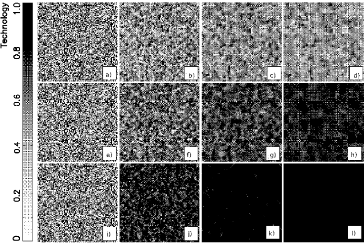
Figure 1: Evolution of cellular automata at different values of $r=a_{2}/a_{1}$: r=1.0, 2.0, 4.0 for the upper, middle and lower rows, respectively. Snapshots were taken at the same times in the rows: $t=1,2,4,15$ from left to right. The gray-scale illustrates the technological level of single agents.

Applying the analytic results Eqs. (10,11) for the specific case of $n=4$, the agents will always copy the 1th, 2nd, 3rd or 4th largest $\tau$ of their local interacting partners when the value of the parameter $r$ falls in the intervals $0<r<1/3$, $1/3<r<1$, $1<r<3$, $3<r$, respectively. Representative examples of the time evolution of a system of size $L=100$ are shown in Fig. 1 for different parameter values in the range $r\geq 1$. (Note that the behavior of the system is symmetric with respect to $r=1$.) Since the system dynamics favors local communities to use the same technology (to be at the same technological level), the agents tend to form clusters with equal $\tau$ at any value of $r$. For the case of $r=1.0$, when being more advanced than the surroundings does not provide any advantages, it can be seen that the system evolves into a frozen cluster structure. The technological level $\tau$ of these clusters covers practically the entire available range with a non-trivial distribution, i.e. communities of low level technologies can survive in the presence of highly advanced ones (see Fig. 1$a,b,c,d$). At $r=2.0$, where more advanced technologies are favored by the agents (locally the second largest $\tau$), the system converges into an almost completely homogeneous state of a relatively high technological level (see Fig. 1$e,f,g,h$). In the simulations, initially clusters of agents with identical $\tau$ grow and finally the entire system evolves into a homogeneous state with all agents adopting the same technology.

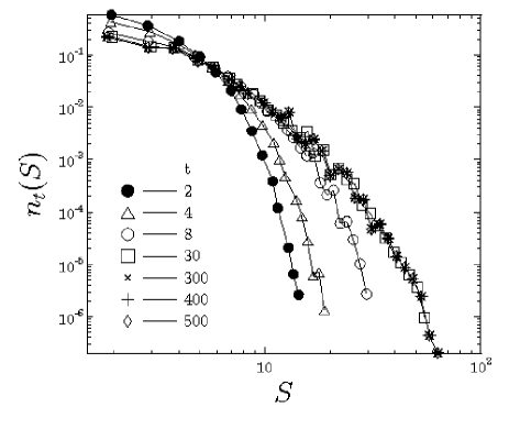
Figure 2: Cluster size distributions $n_{t}(S)$ at different time values $t$ for $r=1$. For $t\geq 30$ the distribution practically does not change, it converges to a rapidly decreasing exponential form.

Locally the agents decide for the second largest $\tau$, and therefore both very low and very high level technologies disappear during the evolution. The gray-scale also illustrates that the limit value of $\tau$ adopted by almost all agents in Fig. 1$h$ falls between 0.8 and 1, i.e. it is smaller than the highest available value $\tau_{max}=1$. To reach the most advanced technologies, $r$ has to surpass the threshold value $r=3$. This regime is illustrated in Fig. 1$i,j,k,l$ for the specific case of $r=4$, where the white color in Fig. 1$l$ implies that the most advanced technology $\tau_{max}=1$ spraw onto the entire lattice.

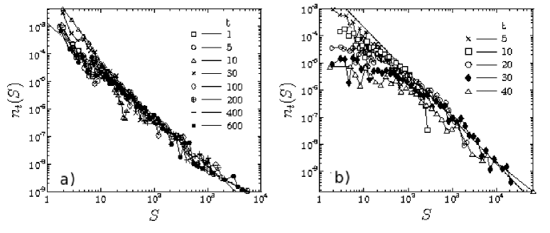
Figure 3: Cluster size distributions $n_{t}(S)$ at different time values $t$ for $r=2$ $(a)$, and $r=4$ $(b)$. At the parameter value $r=2.0$ $(a)$ the distribution $n_{t}(S)$ evolves from an initially rapidly decreasing exponential form to a power law distribution. The power law form proved to be the limit distribution of the system over a broad range of cluster sizes. The value of the exponent $\alpha$ of the fitted power law (straight line in the figure) $\alpha=1.75\pm 0.05$. In both cases $(a)$ and $(b)$ only one cluster remains in the final state, i.e. all the agents have the same technological level. This state is reached through a complex evolution of cluster sizes.

This microscopic restructuring and clusterization process of agents can be characterized by studying the distribution $n_{t}$ of cluster sizes $S$ at different times $t$. A cluster is identified on the lattice as a connected set of agents with the same technological level, where the number of agents defines the cluster size $S$. The numerical results are presented in Figs. 2 and 3 for a system of size $L=1500$. It can be seen in Fig. 2 that for $r=1$, after a few time steps the cluster size distribution converges to a rapidly decreasing exponential form, where even the largest cluster contains a relatively small number of agents. More interesting is the regime $1<r<3$ where agents locally always prefer to adopt the second highest technological level. In this case the initially exponential distribution tends to a power law as time elapses

$$n_{t}(S)\sim S^{-\alpha},$$ (13)

and keeps this functional form over a broad range of time scales (see Fig. 3$a$). The final homogeneous state is reached when small clusters gradually disappear and only one large cluster remains, but the power law distribution remains the same for a long time. The value of the exponent $\alpha$ was determined numerically as $\alpha=1.75\pm 0.05$. For $r>3$ the convergence to the homogeneous final state is faster, but even in this case a power law emerges for intermediate times with the same exponent as before and gradually disappears as the system gets dominated by a single cluster (see Fig. 3$b$).

5 Extreme order statistics and technological progress

In the previous section we have shown that our rejection-adaptation mechanism results in a complex time evolution with local rearrangements which then leads to an overall system change. A very interesting aspect of the model is that the disappearance of certain technologies and proliferation of others may give rise to a global technological progress. In order to give a quantitative characterization of this evolution process, we determined the distribution $p_{t}(\tau)$ of technological levels $\tau$ at different times, and the mean $\left<\tau^{t}\right>$ and standard deviation $\sigma^{t}$ of this distribution

$$\left<\tau^{t}\right>=\frac{1}{N}\sum_{i=1}^{N}\tau_{i}^{t},\ \ \ \ \ \ \qquad\qquad(\sigma^{t})^{2}=\left<\left(\tau^{t}-\left<\tau^{t}\right>\right)^{2}\right>.$$ (14)

Fig. 4 shows that for $r=1$, when higher level technologies do not provide advantages for agents, the distribution $p_{t}(\tau)$ rapidly attains a Gaussian shape.

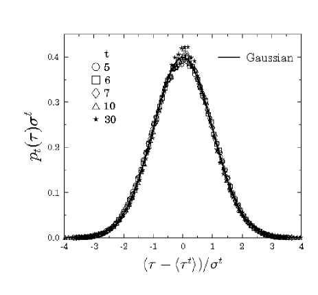
Figure 4: Rescaled distributions of technological levels for $r=1$. The standard Gaussian has a perfect agreement with the numerical results.

In order to demonstrate the validity of the Gaussian form, we plot in Fig. 4 the rescaled distributions $p_{t}(\tau)\sigma^{t}$ as a function of $\left(\tau-\left<\tau^{t}\right>\right)/\sigma^{t}$, which have an excellent agreement with the standard Gaussian $g(x)=1/\sqrt{2\pi}\exp{(-x^{2}/2)}$. The convergence to the Gaussian is very fast, practically after 30-40 iteration steps the system completely forgets its initial uniform state and $p_{t}$ attains the limit distribution. The Gaussian implies that the fraction of agents having very high and very low level technologies both decrease and agents tend to copy technologies in the vicinity of the distribution mean. Consequently, the system does not have any technological progress, the average technological level remains constant during the time evolution, and $\left<\tau^{t}\right>\to 0.5$ (see Fig. 6$a$). In addition, the standard deviation of $p_{t}$ attains a non-zero constant value in the large $t$ limit, $\sigma^{t}\to 0.12$ (Fig. 6$b$).

In contrast, when agents locally prefer to adopt higher level technologies, namely, the largest or the second largest $\tau$ value of the neighborhood on the square lattice, the system undergoes a more complex time evolution involving also extreme order statistics. For $1<r<3$ all the agents adopt the second highest available technology; hence, in a large enough system the distribution of technological levels right after the first iteration step $p_{1}(\tau)$ is the $k=3$ rank extreme distribution $\phi^{k}_{M}$ of $M=4$ variables of uniform distribution.

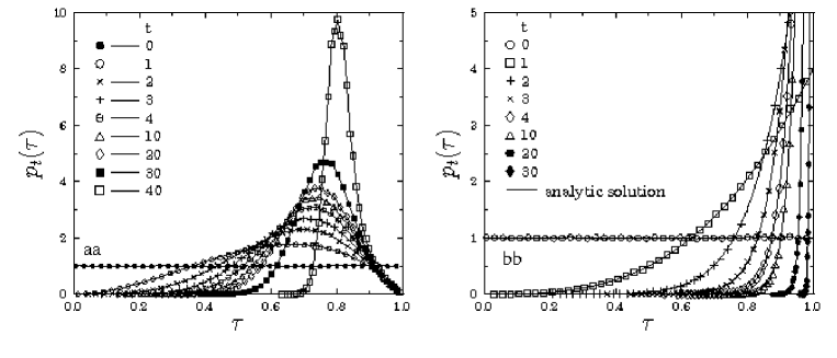
Figure 5: Distribution $p_{t}$ of the technological level $\tau_{i}^{t}$ of agents at different time values $t$ during the evolution of the system. For $r=2$ $(a)$ and $r=4$ $(b)$, the distribution takes an asymmetric form with an increasing average and decreasing standard deviation. In $(a)$ the continuous line of $t=1$ indicates $\phi^{3}_{4}$, furthermore, in $(b)$ the lines of $t=1,2,3,4,5$ stand for $\phi^{4}_{4},\phi^{9}_{9},\phi^{16}_{16},\phi^{25}_{25},\phi^{36}_{36}$, which are in an excellent agreement with the numerical results.

In general, the probability density function $\phi^{k}_{M}(x)$ of the $k$th largest value of $M$ realizations of the random variable $x$ which has a probability density $p(x)$ and a distribution function $P(x)$, can be cast into the form

$$\phi^{k}_{M}(x)=\frac{M!}{(k-1)!(M-k)!}P(x)^{k-1}(1-P(x))^{M-k}p(x).$$ (15)

It can be seen in Fig. 5$a$ that by substituting the initial uniform distribution Eq. (12) into Eq. (15), a perfect agreement is obtained between $\phi^{3}_{4}$ and $p_{1}(\tau)$. Due to the overlap of the local neighborhoods of the lattice sites, however, at higher iteration steps the distributions $p_{t}$ do not follow Eq. (15) when we substitute $\phi_{M}^{k}$ and the corresponding distribution function recursively on the right hand side. By increasing the number of iterations, $p_{t}$ gets narrower and converges to a sharply peaked function as the final homogeneous state is approached (see Fig. 5$a$ and Figs. 1$e,f,g,h$). Consequently, the average value of the technological level increases and converges to a limit value which is smaller than the available maximum $\tau_{max}=1$. The standard deviation goes to zero indicating the homogeneity of the final state (see Fig. 6).

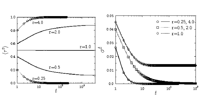
Figure 6: Average technological level $\left<\tau^{t}\right>$ as a function of time $t$ $(left)$, and the standard deviation $\sigma^{t}$ $(right)$. Note the symmetry of the values of $\left<\tau^{t}\right>$ for $r$ and $1/r$ while the corresponding standard deviations fall on the top of each other. For $r=4$ and $r=0.25$ the continuous lines in both figures indicate the analytic results which have an excellent agreement with the numerical calculations.

When the control parameter $r$ becomes larger than $3$, more advanced technologies provide so much benefit that it is always better for agents to adopt the available highest level technology in the local neighborhood. Consequently, $p_{t}(\tau)$ rapidly converges to a sharply peaked form at $\tau_{max}=1$ through extreme order distributions. It is interesting to note that contrary to the case of $1<r<3$, in this regime the distribution $p_{t}$ can be described by the extreme order density function $\phi^{k}_{M}$ Eq. (15) with $k=M$ at any time $t$ by taking into account that $M$ increases as a function of time. We found a recursive formula for the time dependence of the parameter $M$

$$M_{t+1}=M_{t}+5+2(t-1),\qquad\qquad\mbox{with}\qquad\qquad M_{1}=4,$$ (16)

which describes the spreading of successful technologies as a function of time. The continuous lines in Fig. 5$b$ demonstrate the excellent agreement of the above analytic prediction with the numerically obtained distribution functions. Note that due to the symmetry of the system with respect to the parameter value $r=1$, the same holds also for $r<1/3$ with $\phi^{1}_{M}$, where the smallest value ($k=1$) of $M_{t}$ variables given by Eq. (16) is selected. These results imply that the average technological level in these regimes can easily be obtained analytically, i.e. the average of the largest and of the smallest value of $M_{t}$ variables with uniform distribution can be cast into the form

$$\left<\tau_{max}\right>=M_{t}/(M_{t}+1),\ \ \ \ \qquad\qquad\left<\tau_{min}\right>=1/(M_{t}+1).$$ (17)

Substituting the recursive formula of $M_{t}$ into Eq. (17) a perfect agreement is obtained with the numerical results of $\left<\tau^{t}\right>$ presented in Fig. 6$a$.

6 Two providers

By now we have studied the behavior of the system without considering the effect of providers, i.e. all the agents belonged to the same provider. In the following we show that the presence of more than one provider results in a substantial change of the behavior of the system on the meso- and macro-levels.

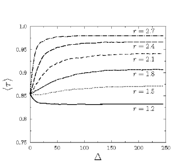
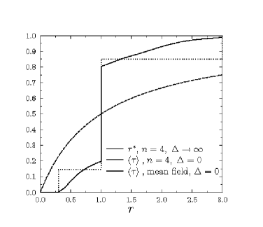
Figure 7: $(left)$ The asymptotic value of the average technological level $\left<\tau\right>=\lim\limits_{t\to\infty}\left<\tau^{t}\right>$ as a function of $\Delta$. For large $\Delta$ the value of $\left<\tau\right>$ converges to a limit value $\tau^{*}$, which depends on $r$. $(right)$ $\tau^{*}$ as a function of $r$ together with the mean field result Eq. (8) and the analytic solution Eqs. (10,11) for $n=4$ obtained at $\Delta=0$.

Let us assume that the initial technological levels are randomly distributed, as before, but in addition a number $n_{1}$ of agents have a provider $S=+1$ and a number $n_{2}$ has another one $S=-1$. The value of $S$ is independent of the technological levels $\tau$. The fraction of agents belonging to the two providers are $p=n_{1}/N$ and $q=1-p=n_{2}/N$, where $N=n_{1}+n_{2}$ is the total number of agents. In the case of an infinite range of interaction among agents (mean field approach) it is straightforward to show that the cost function $C(\tau,\Delta)$ at a finite value of $\Delta$ can be cast into the form

$$C(\tau,\Delta)=C(\tau)+2pq\Delta,$$ (18)

where $C(\tau)$ denotes the mean field cost function Eq. (7) where no providers were considered. Based on the arguments presented in Sec. 3, it follows that after one iteration step the system minimizes the cost function by attaining a uniform state where the median $m$ of the initial distribution of technological levels is copied by all agents and they choose the same provider, namely, the one with the higher initial fraction.

A more interesting (and more realistic) situation occurs when agents of the two providers separate according to the technological levels, i.e. we assume that the $n_{1}$ agents of the $S=-1$ provider have the same technological level $\tau_{1}$, while the $n_{2}$ agents of the $S=+1$ provider have a different one $\tau_{2}$, where $\tau_{1}>\tau_{2}$. We can determine analytically that even if higher level technologies provide advantages ($r>1$), the agents choose the lower level technology $\tau_{2}$ to minimize $C(\tau,\Delta)$ if the excess cost $\Delta$ induced by the interaction of agents of different providers surpass a threshold value

$$\frac{n_{2}a_{2}-n_{1}a_{1}}{n_{1}-n_{2}}(\tau_{1}-\tau_{2})<\Delta.$$ (19)

In the specific case of $n_{1}=n_{2}$ the decision of agents does not depend on the value of $\Delta$, it is only determined by the ratio $r$, as it was the case when there was only one provider present in the system ($n_{1}=0$ or $n_{2}=0$). In local communities (smaller groups of agents) in an extended system such inhomogeneous configurations can frequently occur when two different providers have different number of agents with a clear separation of their technological levels. The above results imply that in such cases $\Delta$ can have a substantial effect on the behavior of the system by modifying the optimal decision of agents with respect to the $\Delta=0$ case. In order to give a quantitative characterization of the effect of $\Delta$ on the micro- and macro-level of the socio-economic system, we carried out computer simulations on a square lattice varying the value of $\Delta$ in a broad range for fixed $r$ parameters. The calculations started from a uniform distribution of technological levels where the two providers had the same fraction $p=0.5$ and $q=0.5$. Computer simulations revealed that as time elapses the average technological level $\left<\tau^{t}\right>$ converges to a limit value which depends both on $r$ and $\Delta$. Fig. 7$a$ presents representative examples of the large time limit of $\left<\tau^{t}\right>$ as a function of $\Delta$ for several different values of $r=a_{2}/a_{1}$ in the range $1<r<3$. It can be seen that at $\Delta=0$ all the curves obtained at different $r$ values start from the same point; however, as $\Delta$ increases the curves split up and the system follow $r$-dependent histories. For very large $\Delta$ the system converges to a limit value $\tau^{*}(r)$ which solely depends on the parameter $r$. Fig. 7$b$ presents a comparison of the $\tau^{*}$ obtained analytically, results of computer simulations performed on a square lattice with $\Delta=0$ (one provider), and the $\Delta\to\infty$ limit values $\tau^{*}(r)$ of $\left<\tau\right>$ as a function of $r$. It is interesting to note that in the regime $r>1$ for most of the cases the presence of two providers makes possible a more intense technological progress, i.e. agents have a higher tendency to adopt technologies closer to the possible maximum compared to the case of a single provider. As $\Delta$ increases the system converges to a steady state where the average technological level is higher than it was with a single provider.

7 Discussion

We presented an agent-based cellular automata model to study the spread of technological achievements in socio-economic systems. Agents of the model can represent individuals or firms which use different level technologies to collaborate with each other. Costs arise due to the incompatibility of technological levels and to different technological providers. Agents can reduce their costs by adopting the technologies and providers of their interacting partners. We showed by analytic calculations and computer simulations that the local adaptation-rejection mechanism of technologies results in a complex time evolution accompanied by microscopic rearrangements of technologies with the possibility of technological progress on the macrolevel. We showed that agents tend to form clusters of equal technological levels. If higher level technologies provide advantages for agents, the system evolves to a homogeneous state but clusters show a power law size distribution for intermediate times. The redistribution of technological levels involves extreme order statistics leading to an overall technological progress of the system. The presence of providers proved to play a substantial role in the time evolution. The competition of providers seems to make the system more sensitive to advantages provided by the higher level technologies and can lead to additional technological progress by forcing the agents to select locally the more advanced technology.

Our model emphasizes the importance of copying in the spreading of technological achievements and considers one of the simplest possible dynamical rules for the decision mechanism. In the model calculations no innovation was considered, i.e., agents could not improve their technological level by locally developing a new technology instead of only taking over of the technology of others. Innovation in the model can be taken into account by randomly selecting agents to increase their technological level by a random amount according to some probability distribution. The generalization of the model in this direction is in progress. Our calculations show also the importance of the structure of local communities in the time evolution of the system which addresses interesting questions for future studies of the model varying the coordination number of the lattice, and on small-world and scale-free network topologies [4, 6, 7, 14, 15]. The emergence of power law size distribution of clusters of agents with equal technological level and the behavior of the exponents on different topologies can be relevant also for applications.

Compared to opinion spreading models like the Sznajd-model [2, 3] and its variants [4, 6, 7], the main difference is that in our case the technological level of agents is a continuous random variable; furthermore, the decision making is not a simple majority rule but involves a minimization procedure. A closer analogy can be found when two providers are considered in the system so that the spreading of a provider could be interpreted as a success of one of two competing “opinions”. Opinion of individuals can also be represented by a continuous real variable which makes possible to study under which conditions consensus, polarization or fragmentation of the system can occur [8]. Such models show more similarities to our spreading model of technologies.

It is interesting to note that our model captures some of the key aspects of the spreading of telecommunication technologies, where for instance mobile phones of different technological levels are used by agents to communicate/interact with each other. In this case, for example, the incompatibility of MMS-capable mobile phones with the older SMS ones may motivate the owner to reject or adopt the dominating technology in his social neighborhood by taking into account the offers of providers of the interacting partners.

References

- [1] W. Weidlich, Sociodynamics: A systematic approach to mathematical modelling in the social sciences, (Dover Publications, Mineola, USA, 2000).
- [2] K. Sznajd-Weron and J. Sznajd, Int. J. Mod. Phys. C 11, 1157 (2000).
- [3] K. Sznajd-Weron and R. Weron, Int. J. Mod. Phys. C 13, 115 (2002).
- [4] D. Stauffer, Journal of Artificial Societies and Social Simulation 5, No. 1, paper 4.
- [5] D. Stauffer, Int. J. Mod. Phys. C 13, 315 (2002).
- [6] A. T. Bernardes, D. Stauffer, and J. Kertész, Eur. Phys. J. B 25, 123 (2002).
- [7] K. Sznajd-Weron, Acta Physica Polonica B 36, 2537 (2005).
- [8] R. Hegselmann and U. Krause, Journal of Artificial Societies and Social Simulations 5, No. 3, paper 2.
- [9] G. Silverberg and B. Verspagen, Journal of Economic Dynamics and Control 29, 225 (2005).
- [10] R. M. Ruiz, E. Albuquerque, L. C. Ribeiro, and A. T. Bernardes, AIP Conf. Proc. 779, 162 (2005).
- [11] A. Arenas, A. Díaz-Guilera, C. J. Pérez, and F. Vega-Redondo, Phys. Rev. E 61, 3466 (2000).
- [12] J.-P. Bouchaud and M. Potters, Theory of financial risk and derivative pricing, (Cambridge University Press, 2000).
- [13] D. Sornette, Critical Phenomena in Natural sciences, (Springer Verlag, Berlin, 2000).
- [14] A. L. Barabasi and R. Albert, Science 286, 509 (1999).
- [15] M. E. J. Newman, SIAM Review 45, 167 (2003).