CALT-68-2667
LPTENS 08/04
SPhT-t08/017
Quantum Wrapped Giant Magnon
Nikolay Gromovα, Sakura Schäfer-Namekiβ and Pedro Vieiraγ
α Service de Physique Théorique, CNRS-URA 2306 C.E.A.-Saclay, F-91191 Gif-sur-Yvette, France; Laboratoire de Physique Théorique de l’Ecole Normale Supérieure et l’Université Paris-VI, Paris, 75231, France; St.Petersburg INP, Gatchina, 188 300, St.Petersburg, Russia
nikgromov@gmail.com
β California Institute of Technology
1200 E California Blvd., Pasadena, CA 91125, USA
ss299@theory.caltech.edu
γ Laboratoire de Physique Théorique de l’Ecole Normale Supérieure et l’Université Paris-VI, Paris, 75231, France; Departamento de Física e Centro de Física do Porto Faculdade de Ciências da Universidade do Porto Rua do Campo Alegre, 687, 4169-007 Porto, Portugal
pedrogvieira@gmail.com
Abstract
Understanding the finite-size corrections to the fundamental excitations of a theory is the first step towards completely solving for the spectrum in finite volume. We compute the leading exponential correction to the quantum energy of the fundamental excitation of the light-cone gauged string in , which is the giant magnon solution. We present two independent ways to obtain this correction: the first approach makes use of the algebraic curve description of the giant magnon. The second relies on the purely field-theoretical Lüscher formulas, which depend on the world-sheet S-matrix. We demonstrate the agreement to all orders in of these approaches, which in particular presents a further test of the S-matrix. We comment on generalizations of this method of computation to other string configurations.
1 Introduction and Summary
In the AdS/CFT correspondence we find ourselves at the point where the S-matrix of [1, 2, 3, 4, 5] is believed to accurately describe the infinite-volume theory, albeit it fails to capture some finite-size effects [6, 7, 8, 9, 10]. The first step towards understanding a theory in finite volume is to compute the leading correction to the dispersion relation of its fundamental excitations. These corrections arise through virtual particles circling in the compact direction, which contribute to the self-energy of physical particles [11]. In this paper we compute the leading quantum finite-size corrections to the fundamental excitation of the string theory.
Tree-level light-cone gauged string theory on is a two-dimensional integrable field theory defined on a worldsheet cylinder of length , where is a large symmetry charge and , with the t’Hooft coupling, plays the role of . In the infinite length limit the fundamental excitations are worldsheet solitons, so-called giant magnons (GM) [12], which transform under the residual extended symmetry [3] and have a non-relativistic dispersion relation111It can also be obtained from a relativistic theory by integrating out some physical degrees of freedom [13].
| (1.1) |
where is the magnon worldsheet momentum. This infinite volume dispersion relation is believed to be exact and almost fixed by symmetry alone [3]. For large
| (1.2) |
where the leading term is the classical energy of the giant magnon and the absence of the term means, that the first quantum correction (or one-loop shift) vanishes for the magnon in infinite volume. This was explicitly checked in [14, 15].
The finite size corrected dispersion relation differs from the infinite volume one by exponentially suppressed terms which can be organized according to world-sheet loop order
The classical finite size corrections to the dispersion relation were computed in222This was also preformed in a more controlled orbifold setup in [16] and generalized for bound states of magnons, called dyonic magnons [17], in [18, 19]. [9] to be
| (1.3) |
where . The first quantum corrections to the dispersion relation (which will in this case be the leading term since the infinite volume contribution vanishes) are computed in this paper and are given by (2.16), of which the first terms in the expansion are333Notice that (2.16) is perfectly well-behaved for . The singularity in (1.4) at is due to the fact that the saddle point approximation breaks down, because the log branch-points approach the saddle point. The approximation (1.4) of (2.16) is valid as long as .
| (1.4) |
where the subleading corrections are of order
As will be explained in section 2 this computation relies solely on the algebraic curve technology [20] and can be easily generalized to other states.
On the other hand it is also known that the leading corrections to the dispersion relation of particles in finite volume is given by Lüscher terms and are a sum of an F-term and a -term contribution depicted in figure 1, which are expressed in terms of the two particle -matrix. The match with the corrections (1.3) and (1.4) provides therefore an important non-trivial check of the AdS/CFT S-matrix [1, 2, 3, 4, 5]. The leading classical correction (1.3) was shown to match the -term computation [10, 18, 19] and we shall show that the leading quantum exponential correction (1.4) is accounted for by the F-term contribution [11, 10]444Note that this formula differs from the one in [10] by the supertrace, i.e. insertion of coming from the fermion loops. We will discuss this point in detail in appendix B.
| (1.5) |
where and are the momenta of the magnon that correspond to the physical particle and to the virtual particle propagating in the loop, respectively, and is determined by the onshell condition .
In section 3 we check that the F-term contribution yields the quantum result to all orders in , which agrees with the algebraic curve result that we obtain in section 2!
2 One-loop energy shift from the algebraic curve
2.1 GM from the algebraic curve
The algebraic curve formalism [20] maps classical string solutions in to a set of eight quasimomenta which define an eight-sheeted Riemann surface. It is convenient to embed the simple giant magnon solution into a family of solutions, called dyonic giant magnons [17], whose infinite volume dispersion relation is given by
where the momentum of the magnon should obviously not be confused with the quasimomenta . For the dyonic magnon reduces to the simple magnon mentioned in the introduction.
In terms of the variables which parametrize the magnon momentum as
| (2.1) |
and are constrained by
| (2.2) |
the infinite volume dispersion relation takes the form
| (2.3) |
The variables are particularly suitable for the curve treatment described below. Notice that for a single magnon, or more generally for which is the case we consider in this paper,
| (2.4) |
and thus .
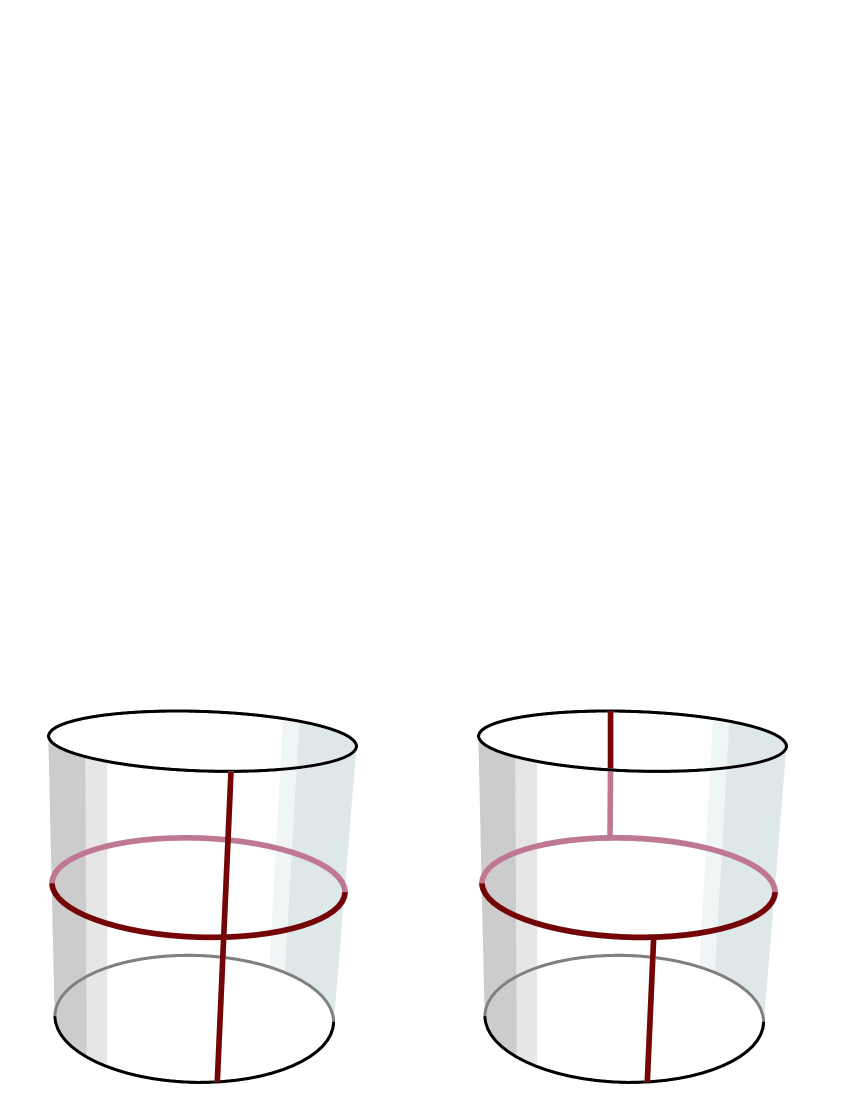
The precise description [21] of the dyonic giant magnon in finite volume is that of a two-cut solution, where the two cuts are very close and thus can be reconnected to form a log-cut condensate with log branch points at , see figure 2. The separation of the two branch-points of the two-cut solution is of the order555This result holds for . The generalization for bigger is also know [19]. . The classical energy of the giant magnon in finite volume differs from the infinite volume log result (2.3) by a contribution of the order [9, 19],
In the same way, if we take into account the precise two-cut structure of the finite volume GM we will also find a contribution to the fluctuation energies – and therefore to the one-loop shift – with the same exponential suppression. However, as already anticipated in the introduction, there are more important corrections (1.4) of the order
which simply come from the fact that in order to compute the ground state energy in finite volume, we should sum over the fluctuation energy mode number instead of integrating over the momenta of the quantum fluctuations. Thus, to compute the leading order quantum finite size corrections we can work with the log cut description [22] of the giant magnon solution for which [22, 15]
| (2.5) |
The twists in the quasimomenta [23] are necessary because for a single magnon we cannot satisfy the usual periodic boundary conditions. The usual orbifold treatment [24, 25, 16] selects the twists
| (2.6) |
as reviewed in appendix .
We shall now study the quantum fluctuations around this classical solution. By perturbing the quasimomenta via the addition of extra poles we can compute the fluctuation energies around this classical solution [26]. The poles are shared by quasimomenta and and the different possible choices of quasimomenta correspond to different string polarizations, namely
| (2.7) | |||||
| (2.8) | |||||
| (2.10) | |||||
Moreover each quantum fluctuation has a mode number , which will dictate where the corresponding pole outside the unit circle will be located through
| (2.11) |
In this way we can find the semi-classical spectrum of fluctuations around the GM solution which reads
| (2.12) |
The result of the perturbation of the quasimomenta, which is explicitly presented in appendix , is that all fluctuation energies are given by the same function, when expressed in terms of the position of the poles , that is for all . The function is given by
| (2.13) |
Notice that this does not mean that the fluctuation energies are all the same, when expressed in terms of the mode number , because for each string polarization the map is different and given by (2.11).
Formula (2.13) for the fluctuation energies has a nice physical interpretation which can indeed be used as an alternative (and simpler) derivation of this expression. Namely, we know [20, 26] that the quantum fluctuations located at in the algebraic curve carry energy and momentum666An extra excitation is still described by formulas (2.1,2.2,2.3) with . Quantum fluctuations in the scaling limit have momentum so that are then given by , where is the position of the quantum fluctuation in the algebraic curve (or the position of the Bethe roots in the AdS/CFT Bethe ansatz [2]). Thus in this limit (2.14) follows from (2.1,2.3).
| (2.14) |
When we add a fluctuation the energy is not simply given by because the fluctuation will backreact and slightly modify the classical background. The correct energy shift is then given by the energy of the fluctuation plus the backreaction of the the giant magnon,
where is the shift in the momentum of the magnon due to the presence of the fluctuation, and by momentum conservation it equals . Since
formula (2.13) follows.
2.2 GM one-loop shift
The ground state energy around a classical solution, known as the one-loop energy shift, is given by the graded sum over one half of each fluctuation energy:
The sum extends over all polarizations as listed in (2.7). It is convenient [7, 27] to rewrite this sum over as an integral
where the contour encircles the real axis. Next, for each polarization we change the variables to via (2.11) so that the integration over maps to contours which encircle the fluctuation positions located outside the unit circle . For a generic polarization , we can deform this contour777Notice that the orientation of the contour flips in the process. in the plane and obtain an integral over the unit circle plus an integral over the eventual cuts of the classical solution, in this case the log cut in (2.5). Up to exponentially suppressed terms, which we are now focussing on, these two contributions were universally analyzed in [27] and [23] respectively. The possible contribution from the integral over the log cut is given by the log branch points , which become pole terms when plugged into the integral in the plane (see (2.16) below). It is easy to see that this contribution enters as
and is subleading compared with the contribution coming from the integral over the unit circle which we will now consider. We shall however return to this point in the discussions.
We therefore have
On the upper/lower half of the unit circle, , the quasimomenta are large and
| (2.15) |
Picking the leading term we get a zero result for the one-loop shift since
which is precisely the vanishing result derived in [22] and mentioned in the introduction in (1.2). The leading exponential correction to the one-loop shift - which in this case turns out to be the leading result for this quantity - is obtained by picking the second term of the expansion of the cotangent. After an integration by parts we find888The extra factor of appearing comes from keeping the integration over the upper half circle only.
| (2.16) |
where is given by (2.13). From (2.5) using that for a single giant magnon including the twists given in (2.6), we obtain
| (2.17) |
It is clear that this expression is suppressed by which is indeed leading compared to the effects we have discarded so far. The expansion (1.4) mentioned in the introduction is trivially obtained by expanding around the saddle point .
3 Lüscher F-term
The Lüscher F-term is given by (1.5). We will now evaluate this for a single magnon and show that it gives rise to the same one-loop leading exponential correction to all orders in as in (2.16). Physically, the F-term computes the correction to the energy of the giant magnon with momentum by a virtual particle with momentum circulating in the compact worldsheet direction. Due to the supertrace in (1.5), whose origin we discuss in appendix B, the only contribution comes from the S-matrix part.
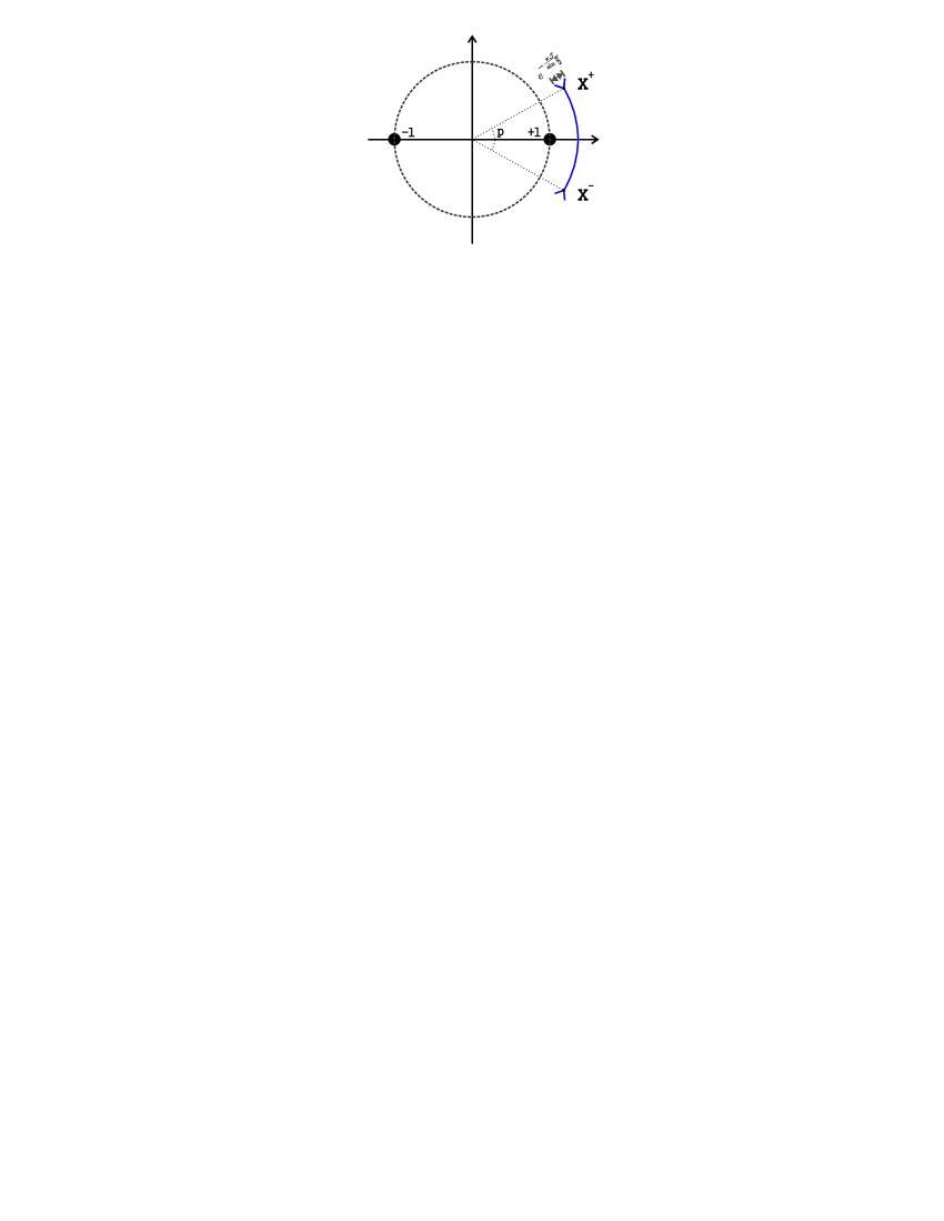
The momenta of both the physical particle, , and the virtual particle, , appear in the S-matrix through and . As mentioned before, the former lie in the unit circle with
| (3.1) |
As for the virtual particle [10] so that for we have and thus
| (3.2) |
In terms of we have
The contour over the real axis is mapped to the upper half of the unit circle in the plane and the saddle point of the F-term, at , is mapped to , which is the same saddle point we found at the end of the previous section.
Moreover
so that the F-term (1.5) becomes
| (3.3) |
where is the same function (2.13) which appeared in the curve computation! Finally, using the explicit form of the AdS/CFT S-matrix in this setup, which we discuss in Appendix B, we find that this contributes for the particular kinematics (3.1,3.2) as
| (3.4) |
Thus, combining (3.3) and (3.4) we find precisely the integral (2.16) appearing in the curve computation. Since our match is at the level of the integrals we have an all order (in ) agreement between both computations!
4 Discussion and Future Work
The ground state energy for the giant magnon in finite volume is an exponentially suppressed quantity which appears to have an expansion
where each prefactor is a nontrivial function of and . We computed the leading contribution, namely , and checked that it can be reproduced through an F-term contribution (cf. figure 1).
Depending on the value of the momentum , the next-to-leading order coefficient is or . The latter has the typical exponential suppression we find from the term computation [10] and will surely come from the next to leading correction to the results in [10]. From the algebraic curve point of view this correction could come from two different places. Firstly, from the discrepancy between the log cut description [22] used here and the true giant magnon in finite volume described in [21] which is in fact a two-cut solution (cf. figure 2). Secondly from the integral of the fluctuation energies over the cuts of the classical solution as discussed in section 2.2. It would be very interesting to match the curve and the -term results.
As for the the coefficients , they come from the subleading terms in the expansion (2.15) of the cotangent, and therefore can be trivially computed from the curve point of view to be
| (4.1) |
where is the upper half of the unit circle, the giant magnon quasimomenta (2.5) and the flucuation energies (2.13).
The remaining coefficients will most likely come from virtual processes with virtual particle loops in addition to splits into two on-shell particles. It would be extremely instructive to generalize the - and F-term results of Lüscher to allow for such processes. The curve computation might serve as an important guide since in principle these exponential corrections can be independently computed in this formalism. It would be interesting to try to find a more general integrable structure behind these contributions, eventually using the already known as potential guidelines.
Another possible direction would be to compute the two (worldsheet) loop correction to the dispersion relation of the giant magnon. The leading order term will be of the order and will come from the next-to-leading expansion in of the F-term obtained in this paper. This computation would provide a two-loop prediction for the dispersion relation of the giant magnon in finite volume which would be interesting to check against a direct two-loop computation in the spirit of [28].
Yet another interesting next step is to consider more physical string solutions with zero total momentum. The simplest example is to consider two magnons with momenta and (this setup was studied classically in [19]). The computations in the sections above can be trivially generalized both in the curve and in the F-term setup and yield for the leading contribution
| (4.2) |
for the one-loop shift of the two magnon system in finite volume. Here . As an expansion in large we find therefore the leading terms
Finally it would be interesting to try to extend our computations to the most general setup possible including, not only the more general dyonic giant magnons, but also generic classical solutions. For solutions moving in , when is much larger than all the other filling fractions the leading exponential corrections will behave like
since the sum over frequencies, when transformed into an integral in the plane will be dominated by a saddle point at where the quasimomenta are, to leading order,
This is in agreement with the findings in [7]. We shall address these issues in a forthcoming publication [29] where we study the F-term vs. curve approach for generic classical solutions.
Acknowledgements
We would like to thank T. Dimofte, A. Mikhailov, J. Minahan, R. Janik, V. Kazakov, and K. Zarembo for many useful discussions. The work of N.G. was partially supported by French Government PhD fellowship, by RSGSS-1124.2003.2 and by RFFI project grant 06-02-16786. NG was also partly supported by ANR grant INT-AdS/CFT (contract ANR36ADSCSTZ). S.S.-N. is supported by a Caltech John A. McCone postdoctoral fellowship. P. V. is funded by the Fundação para a Ciência e Tecnologia fellowship SFRH/BD/17959/2004/0WA9. We would like to thank the Isaac Newton Institute in Cambridge for an inspiring atmosphere during the SIS workshop.
Appendix A Details for algebraic curve computation
To find the fluctuation energies we perturb the quasimomenta (2.5) so that . The perturbation are fixed by some simple analytical properties of . We add fluctuations with mode number and polarization . This means must have poles at position
with residue
| (A.1) |
where the signs of the residues are
and
Analogously to the original quasimomenta, the fluctuation can have poles at but those must be synchronized
| (A.2) |
due to the Virasoro constraints. There is also an symmetry inherited from the coset structure of the connection, which for the fluctuations imposes
| (A.3) |
The large asymptotics of the quasimomenta are fixed by the global charges of the theory and are
| (A.20) |
Finally the fluctuations will backreact onto the original solution thus shifting the log cut. Therefore close to the quasimomenta will behave like
| (A.21) |
This is the only particularity of the GM when compared to the solutions studied in [26] where close to the branch points of the classical solution we had .
The analytical properties (A.1,A.2,A.3,A.20,A.21) are obviously enough to fix the functions completely – the steps involved mimicking the ones in [26] closely. We find
where the symmetry fixes
while the large asymptotics yields
These conditions completely fix and require moreover which is nothing but the string level matching condition. For the result is given by (2.12) with as in (2.13).
Appendix B Details for F-term computation
We now specify all the terms appearing in the F-term integral (1.5). For our purposes it is enough to consider the AFS-part [30] of the S-matrix [3, 5, 4]. The one-loop Hernandez-Lopez correction would contribute one order higher in .
We should now also comment on the insertion in (1.5). In theories with bosonic and fermionic degrees of freedom, the self-energy corrections, which are computed by the Lüscher formulas, enter with different signs depending on the statistics of the particles in the loop. This arises solely through the fermion contractions and was also observed in applications of the Lüscher formula to chiral perturbation theory in [31] – see e.g. formula (10) in the first reference in [31]. In the self-energy diagrams , and of [11, 10], we have external lines given by the giant magnon, so that the statistics of the internal contributions can be summarized by . This results in particular in the insertion of in (1.5) and the contribution from the S-matrix is then999Note the different sign of the fermion term compared to [10, 18], which is due to the supertrace. Note, that for the -term computation of [10, 18] this sign was irrelevant as in their limit the term did not contribute. Also, the fact that the supertrace removes the term in (for supersymmetric theories) was neglected there, which however was again irrelevant for the purpose of the evaluation of residues that is necessary for the -term. However all these points are crucial for the F-term computation in this paper.:
| (B.1) |
where
In the scaling limit (3.2) we find
and
For a simple GM we have and reduces to the simple result (3.4) in the main text.
Appendix C Twists – orbifolding the GM
In this appendix we closely follow the approach of [24, 16, 23] and most importantly the one of [25]. The giant magnon solution is a worldsheet soliton whose target space picture is that of a string moving in with endpoints located on the equator and moving with the speed of light so that [12]
where is the rescaled worldsheet space coordinate which ranges from to in the infinite spin limit. Thus, to properly treat the giant magnon we must replace the usual periodic boundary condition by
| (C.1) |
with all the other coordinates and periodic. The new boundary conditions (C.1) can be incorporated by a orbifold with
which for the Higher Dynkin diagram Bethe equations used in [25, 2, 23] amounts to adding a phase
to the RHS of the Bethe equations (in [23] these twists were written as , see equation (6.1) there). The seven twists are given by
which in the language of [23] means
thus explaining the choice (2.6) in the main text.
References
- [1] M. Staudacher, The factorized S-matrix of CFT/AdS, JHEP 05 (2005) 054, [hep-th/0412188].
- [2] N. Beisert and M. Staudacher, Long-range Bethe ansätze for gauge theory and strings, Nucl. Phys. B727 (2005) 1–62, [hep-th/0504190].
- [3] N. Beisert, The dynamic S-matrix, hep-th/0511082.
- [4] N. Beisert, R. Hernandez, and E. Lopez, A crossing-symmetric phase for AdS(5) x S(5) strings, JHEP 11 (2006) 070, [hep-th/0609044]. N. Beisert, B. Eden, and M. Staudacher, Transcendentality and crossing, J. Stat. Mech. 0701 (2007) P021, [hep-th/0610251].
- [5] G. Arutyunov, S. Frolov, and M. Zamaklar, The Zamolodchikov-Faddeev algebra for AdS(5) x S(5) superstring, JHEP 04 (2007) 002, [hep-th/0612229].
- [6] J. Ambjorn, R. A. Janik, and C. Kristjansen, Wrapping interactions and a new source of corrections to the spin-chain / string duality, Nucl. Phys. B736 (2006) 288–301, [hep-th/0510171].
- [7] S. Schafer-Nameki, Exact expressions for quantum corrections to spinning strings, Phys. Lett. B639 (2006) 571–578, [hep-th/0602214]
- [8] S. Schafer-Nameki and M. Zamaklar, Stringy sums and corrections to the quantum string Bethe ansatz, JHEP 10 (2005) 044, [hep-th/0509096] S. Schafer-Nameki, M. Zamaklar, and K. Zarembo, How accurate is the quantum string Bethe ansatz?, JHEP 12 (2006) 020, [hep-th/0610250] A. V. Kotikov, L. N. Lipatov, A. Rej, M. Staudacher, and V. N. Velizhanin, Dressing and wrapping, J. Stat. Mech. 0710 (2007) P10003, [arXiv:0704.3586 [hep-th]]. G. Arutyunov and S. Frolov, On String S-matrix, Bound States and TBA, JHEP 0712 (2007) 024 [arXiv:0710.1568 [hep-th]]
- [9] G. Arutyunov, S. Frolov, and M. Zamaklar, Finite-size effects from giant magnons, Nucl. Phys. B778 (2007) 1–35, [hep-th/0606126].
- [10] R. A. Janik and T. Lukowski, Wrapping interactions at strong coupling – the giant magnon, Phys. Rev. D76 (2007) 126008, [arXiv:0708.2208 [hep-th]].
- [11] M. Luscher, Volume dependence of the energy spectrum in massive quantum field theories. 1. Stable particle states, Commun. Math. Phys. 104 (1986) 177 M. Luscher, Volume dependence of the energy spectrum in massive quantum field theories. 2. Scattering states, Commun. Math. Phys. 105 (1986) 153–188 T. R. Klassen and E. Melzer, On the relation between scattering amplitudes and finite size mass corrections in QFT, Nucl. Phys. B362 (1991) 329–388.
- [12] D. M. Hofman and J. M. Maldacena, Giant magnons, J. Phys. A39 (2006) 13095–13118, [hep-th/0604135].
- [13] N. Gromov, V. Kazakov, K. Sakai and P. Vieira, Strings as multi-particle states of quantum sigma-models, Nucl. Phys. B 764 (2007) 15 [hep-th/0603043] N. Gromov and V. Kazakov, Asymptotic Bethe ansatz from string sigma model on S(3) x R, Nucl. Phys. B 780, 143 (2007) [hep-th/0605026].
- [14] G. Papathanasiou and M. Spradlin, Semiclassical quantization of the giant magnon, JHEP 06 (2007) 032, [arXiv:0704.2389 [hep-th]].
- [15] H.-Y. Chen, N. Dorey, and R. F. Lima Matos, Quantum scattering of giant magnons, JHEP 09 (2007) 106, [arXiv:0707.0668 [hep-th]].
- [16] D. Astolfi, V. Forini, G. Grignani, and G. W. Semenoff, Gauge invariant finite size spectrum of the giant magnon, Phys. Lett. B651 (2007) 329–335, [hep-th/0702043].
- [17] N. Dorey, Magnon bound states and the AdS/CFT correspondence, J. Phys. A39 (2006) 13119–13128, [hep-th/0604175].
- [18] Y. Hatsuda and R. Suzuki, Finite-size effects for dyonic giant magnons, arXiv:0801.0747 [hep-th].
- [19] J. A. Minahan and O. O. Sax, Finite size effects for giant magnons on physical strings, arXiv:0801.2064 [hep-th].
- [20] V. A. Kazakov, A. Marshakov, J. A. Minahan, and K. Zarembo, Classical / quantum integrability in AdS/CFT, JHEP 05 (2004) 024, [hep-th/0402207] V. A. Kazakov and K. Zarembo, Classical / quantum integrability in non-compact sector of AdS/CFT, JHEP 10 (2004) 060, [hep-th/0410105] N. Beisert, V. A. Kazakov, and K. Sakai, Algebraic curve for the SO(6) sector of AdS/CFT, Commun. Math. Phys. 263 (2006) 611–657, [hep-th/0410253] S. Schafer-Nameki, The algebraic curve of 1-loop planar N = 4 SYM, Nucl. Phys. B714 (2005) 3–29, [hep-th/0412254]. N. Beisert, V. A. Kazakov, K. Sakai, and K. Zarembo, The algebraic curve of classical superstrings on AdS(5) x S(5), Commun. Math. Phys. 263 (2006) 659–710, [hep-th/0502226]. N. Beisert, V. A. Kazakov, K. Sakai, and K. Zarembo, Complete spectrum of long operators in N = 4 SYM at one loop, JHEP 07 (2005) 030, [hep-th/0503200].
- [21] B. Vicedo, Giant magnons and singular curves, JHEP 12 (2007) 078, [hep-th/0703180].
- [22] J. A. Minahan, A. Tirziu, and A. A. Tseytlin, Infinite spin limit of semiclassical string states, JHEP 08 (2006) 049, [hep-th/0606145].
- [23] N. Gromov and P. Vieira, Complete 1-loop test of AdS/CFT, arXiv:0709.3487 [hep-th].
- [24] K. Ideguchi, Semiclassical strings on AdS(5) x S(5)/Z(M) and operators in orbifold field theories, JHEP 09 (2004) 008, [hep-th/0408014] A. Solovyov, Bethe ansatz equations for general orbifolds of N=4 SYM, arXiv:0711.1697 [hep-th].
- [25] N. Beisert and R. Roiban, The Bethe ansatz for Z(S) orbifolds of N = 4 super Yang- Mills theory, JHEP 11 (2005) 037, [hep-th/0510209].
- [26] N. Gromov and P. Vieira, The AdS(5) x S(5) superstring quantum spectrum from the algebraic curve, Nucl. Phys. B789 (2008) 175–208, [hep-th/0703191].
- [27] N. Gromov and P. Vieira, Constructing the AdS/CFT dressing factor, Nucl. Phys. B790 (2008) 72–88, [hep-th/0703266].
- [28] R. Roiban, A. Tirziu, and A. A. Tseytlin, Two-loop world-sheet corrections in AdS(5)xS(5) superstring, JHEP 07 (2007) 056, [arXiv:0704.3638 [hep-th]] R. Roiban and A. A. Tseytlin, Strong-coupling expansion of cusp anomaly from quantum superstring, JHEP 11 (2007) 016, [arXiv:0709.0681 [hep-th]] R. Roiban and A. A. Tseytlin, Spinning superstrings at two loops: strong-coupling corrections to dimensions of large-twist SYM operators, arXiv:0712.2479 [hep-th].
- [29] N. Gromov, S. Schafer-Nameki, and P. Vieira, in progress.
- [30] G. Arutyunov, S. Frolov, and M. Staudacher, Bethe ansatz for quantum strings, JHEP 10 (2004) 016, [hep-th/0406256].
- [31] Y. Koma and M. Koma, On the finite size mass shift formula for stable particles, Nucl. Phys. B 713 (2005) 575 [hep-lat/0406034] Finite size mass shift formula for stable particles revisited, Nucl. Phys. Proc. Suppl. 140 (2005) 329 [hep-lat/0409002] More on the finite size mass shift formula for stable particles, [hep-lat/0504009]