Inhomogeneous Light Shift Effects on Atomic Quantum State Evolution in Non-Destructive Measurements

Abstract

Various parameters of a trapped collection of cold and ultracold atoms can be determined non–destructively by measuring the phase shift of an off–resonant probe beam, caused by the state dependent index of refraction of the atoms. The dispersive light–atom interaction, however, gives rise to a differential light shift (AC Stark shift) between the atomic states which, for a nonuniform probe intensity distribution, causes an inhomogeneous dephasing between the atoms. In this paper, we investigate the effects of this inhomogeneous light shift in non–destructive measurement schemes. We interpret our experimental data on dispersively probed Rabi oscillations and Ramsey fringes in terms of a simple light shift model which is shown to describe the observed behavior well. Furthermore, we show that by using spin echo techniques, the inhomogeneous phase shift distribution between the two clock levels can be reversed. 32.80.-tphoton–atom interactions and 03.65.Yzdecoherence, quantum mechanics and 06.30.Ftclocks

1 Introduction

Resonant absorption and fluorescence measurements have been employed extensively in recent years to probe the properties of cold and ultracold atomic gasses. For example, Bose Einstein condensates are typically recorded in absorption imaging. Resonant light–atom interaction, however, destroys initial sample properties such as coherences between the internal states of the atoms. Phase contrast imaging using off resonant light offers an alternative, non-destructive means of probing, which has proven viable, e.g. in following the evolution of the vector magnetization density with repeated imaging of the same atomic sample [1]. In general, such measurements can be used to probe the evolution of the sample density [2] and the internal state populations [3, 4, 5], When fulfilling the requirements for Quantum Nondemolition (QND) measurements [6], the dispersive interaction, furthermore, provides a vehicle for quantum state generation in ensembles of atoms, for example for the generation of spin squeezed and entangled states of atoms [7, 8]. Such QND measurements form a basis for a number of protocols in the field of quantum information science [9, 10] such as quantum memory [11], and quantum teleportation [12].
Non-destructive measurements could potentially prove useful in the operation of atomic clocks. The accuracy of state–of–the art clocks is presently limited by the projection noise [13], which arises from the probabilistic uncertainty associated with a projective measurement of independent particles in a quantum mechanical superposition state. To reduce this uncertainty, one can explore the possibility of creating so called squeezed states [14, 15, 16, 17] via QND measurements, where the particles are no longer independent but rather non–classically correlated (entangled). Furthermore, in approaches like optical lattice clocks, a way of improving the signal-to-noise ratio, which directly enters into the frequency stability, is to increase the duty cycle of sample preparation relative to the actual interrogation time [18, 19, 20]. This can be achieved by using non–destructive probing schemes where the trapped sample, once prepared, is reused several times during the lifetime of the trap.
While off–resonant probing may lead to negligible decoherence due to spontaneous photon scattering, the dispersive light–atom interaction inevitable affects the atomic states via the AC–Stark shift. The influence of this light shift in Caesium fountain clocks, where it is induced by a homogeneously distributed off–resonant light field, has been studied in [21]. The assessment of such effects and the ability to account for them, is of major importance when employing non–destructive probing schemes in practical applications.
We have constructed a Caesium atomic clock, using a dipole trapped cold sample. Our eventual and primary goal is to demonstrate pseudo–spin squeezing of the clock transition via a QND measurement [16]. To that end, we read out the population of the clock states non–destructively by measuring the phase shift acquired by probe light due to the off–resonant index of refraction of the atomic medium. The phase shift of the probe light is measured with a Mach–Zehnder interferometer, operating close to the standard quantum limit [5]. Since our readout beam has a Gaussian intensity profile, the interrogation of the (inhomogeneous) sample induces an inhomogeneous light shift across the atomic sample, which finally is detected with a non–uniform detection efficiency. In the present paper we analyze these inhomogeneous effects by studying the evolution of clock–state Rabi oscillations, and we perform Ramsey spectroscopy measurements to further characterize the dephasing. We finally investigate the reversibility of the probe–introduced dephasing with spin echo techniques.

2 Experimental setup

2.1 Framework

The system we are considering is the standard microwave clock transition $6S_{1/2}(F=3,m_{F}=0)\equiv|3\rangle\leftrightarrow 6S_{1/2}(F=4,m_{F}=0)\equiv|4\rangle$ [22] in cold Cs–atoms. Earlier versions of the experimental setup have been described in [16, 2, 5]. A schematic drawing of the setup is shown in Fig. 1.

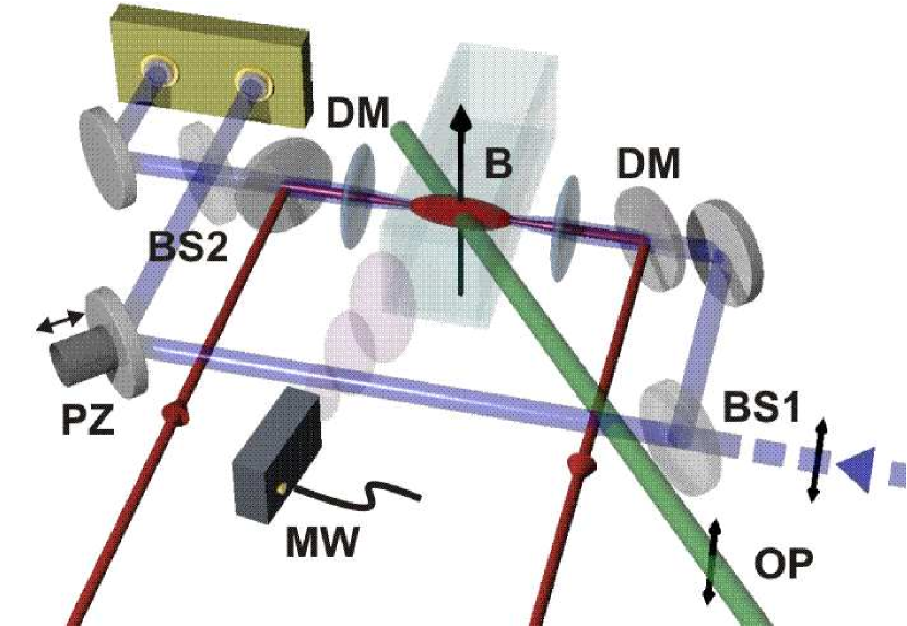
Figure 1: Schematic drawing of the experimental setup. A probe laser beam enters the interferometer via a port of the beam splitter BS1. One part of the beam propagates through the Cs atoms confined by a dipole trap, as they interact with the radiation field of the microwave source MW. The dipole beam is coupled into the probe arm via two dichroic mirrors DM. The other part of the beam propagates on a reference path with no atoms. The beams are recombined at the beam splitter BS2 and the phase shift from the atoms is detected as the differential signal of detectors at the two output ports of BS2. The geometrical path length difference of the interferometer arms is stabilized with a piezoelectric element PZ. B shows the direction of the magnetic guiding field and OP the two counter–propagating optical pumping beams.

A typical experimental cycle starts by loading Cs atoms into a magneto–optical trap and after a sub-Doppler cooling stage, we transfer about $10^{5}$ Cs atoms with a temperature of $\sim 15\,\mu$K into a single beam, far-off resonance dipole trap [23]. A diode pumped Yb:YAG disk laser at 1032 nm produces 4 W of dipole trapping beam, focussed down to a waist of about $50\,\mu$m. To initialize the atomic ensemble to one of the clock states, a homogeneous, magnetic guiding field of $\sim 1$ Gauss is applied and the atoms are subsequently optically pumped into the $6S_{1/2}(F=4,m_{F}=0)$ ground state by simultaneously applying linearly polarized light to the $6S_{1/2}(F=4)\to 6P_{3/2}(F^{\prime}=4)$ and $6S_{1/2}(F=3)\to 6P_{3/2}(F^{\prime}=4)$ transitions [24]. A schematic level diagram of Cs is shown in Fig. 2 for reference.

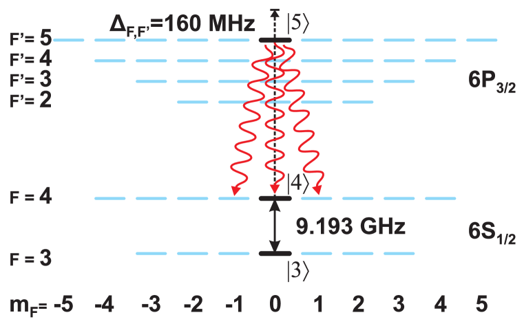
Figure 2: Schematic level diagram indicating a resonant drive between the states $|3\rangle$ and $|4\rangle$ as well as dispersive (off-resonant) coupling between the states $|4\rangle$ and $|5\rangle$. In the experiment $|3\rangle$ is the $6S_{1/2}(F=3,m_{F}=0)$ Cs clock state, $|4\rangle$ is the $6S_{1/2}(F=4,m_{F}=0)$ clock state, and $|5\rangle$ is the $6P_{3/2}(F^{\prime}=5,m_{F}=0)$ state. We also indicate three possible spontaneous photon scattering channels.

The efficiency of the optical pumping is limited to about 80% by off–resonant excitations, magnetic background field fluctuations, polarization impurities and the narrow bandwidth of the pumping laser [25]. To achieve a purer ensemble, where all atoms populate a single clock state, we first transfer the population in the $|4\rangle$ state to the $|3\rangle$ clock state with a resonant microwave $\pi$–pulse. The remaining atoms in $6S_{1/2}(F=4,m_{F}\neq 0)$ are then expelled from the trap with the resonant light on the cycling $6S_{1/2}(F=4)\leftrightarrow 6P_{3/2}(F^{\prime}=5)$ transition. In this way we obtain an ensemble with $\gtrsim 99\,\%$ purity.
To drive a coherent evolution of the clock state populations, $|3\rangle\leftrightarrow|4\rangle$, we apply a linearly polarized microwave field with a frequency of $\sim 9.2$ GHz with various durations and powers to the atoms. The microwave field is generated by a HP8341B precision synthesizer and amplified with a solid state amplifier to 1W. To stabilize the power, we split a portion of the microwave power into a solid state detector and feed the signal directly back onto the synthesizer’s external stabilization input. Pulse shaping is done with a HP4720A pulse modulator inserted after the feedback loop and the resulting microwave pulses are directed into the vacuum cell via a cut–to–size rectangular waveguide. The microwaves produce the Rabi flopping, characteristic to a two level system strongly driven with a near resonant coupling field [26].
To read out the population of the ensemble in the state $|4\rangle$ non–destructively, we measure the phase shift of the probe light [16, 2] caused by the state dependent refractive index of atoms [27]:

$$\Delta\phi=\frac{5}{36}\phi_{0}N_{|4\rangle}\frac{(\gamma/2)\Delta_{F,F^{\prime}}}{\Delta_{F,F^{\prime}}^{2}+(\gamma/2)^{2}},$$ (1)

where $\phi_{0}=3l\lambda^{2}/\pi V$, $N_{|4\rangle}$ is the number of atoms in the ${|4\rangle}$ clock state, $\Delta_{F,F^{\prime}}$ is the detuning of the probe light from the $6S_{1/2}(F=4)\to 6P_{3/2}(F^{\prime}=5)$ transition, $\lambda$ is the wavelength of the probe light, $\gamma$ is the linewidth of the transition, and $l$ is the length and $V$ the volume of the sample. To obtain the reduced form of the phase shift, given in equation (1), we have assumed a pure sample in ${|4\rangle}$ and neglected couplings to the $6P_{3/2}(F^{\prime}\neq 5$) levels [5].
Experimentally, the phase shift of the probe light is recorded by placing the ensemble into one arm of a Mach–Zehnder interferometer and detecting the two interferometer outputs with two photodiodes whose outputs are fed into a low noise AC integrating photoamplifier. The differential output of the detector is directly digitized with a storage oscilloscope, saved to disk and the recorded pulses are numerically integrated afterwards. For the probe light, we arrange the detuning $\Delta_{F,F^{\prime}}=+160\,$MHz such that we get a considerable phase shift of up to half a radian due to the presence of atoms in the interferometer, while keeping the probability of spontaneous photon scattering low. With $\sim 10^{5}$ photons in one probe pulse, the spontaneous scattering probability per atom is around $0.05$ %. The pulses are generated using a standard acousto–optical modulator and with typical durations between 200 ns and a few microseconds. To clean the transverse mode of the beam before entering the interferometer, the pulsed probe–beam is coupled into an optical fibre. The path length difference of the two interferometer arms is actively stabilized against thermal drifts and acoustic noise by applying feedback to one of the folding mirrors. The error signal for the feedback is obtained by matching a weak, pulsed locking laser with $\sim 1.5\,\mu$W equivalent DC power into the mode cleaning fibre used for the probe pulses, and demodulating the signal from the photo–receiver. We usually lock the interferometer to the white light position, where both arms have the same optical path length. To eliminate an influence of the locking laser onto the atoms, its wavelength is $\sim 20$ nm blue detuned from the $6S_{1/2}\to 6P_{3/2}$ transition. Due to its detuning, the locking beam is not affected by the presence of atoms so that the geometrical path length can be fixed irrespectively of the atomic state and density.

Using our non–destructive probing scheme, we can follow the evolution of the atomic ensemble quantum state when subjected to external fields. More specifically, we measure the population in the $|4\rangle$ clock state. Figure 3a shows a typical recording of microwave induced Rabi oscillations on the clock transition. A constant resonant microwave driving field is applied while the atomic ensemble is probed every $10.3\,\mu$s with $0.2\,\mu$s optical probe pulses, corresponding to $\sim 10^{5}$ photons per pulse. The figure represents an average of 10 experimental runs each sampling the atoms $\sim 500$ times [5]. From a fit to the data, assuming a cosine function with exponentially decaying envelope, we extract a time constant of $\tau=3.0$ ms.

2.2 Motivation

Some care is required when describing dispersive probing as non–destructive. In our case, the probing is non–destructive in the sense that the spontaneous photon scattering is kept very low. With the exception of the case where the ensemble is in one of the eigenstates $|3\rangle$ or $|4\rangle$, spontaneous scattering events destroy coherences irreversibly [28], i.e. project superposition states onto eigenstates. However, even for negligible spontaneous scattering, the atomic quantum state will be affected: The dispersive light–atom interaction will introduce a phase shift between the atomic states $|3\rangle$ and $|4\rangle$ due to the light shift caused by the probe [21]. When probing Rabi oscillations non-destructively, we observe a very distinct change in the envelope when changing the probe power rather moderately. Figure 3b shows two traces of Rabi

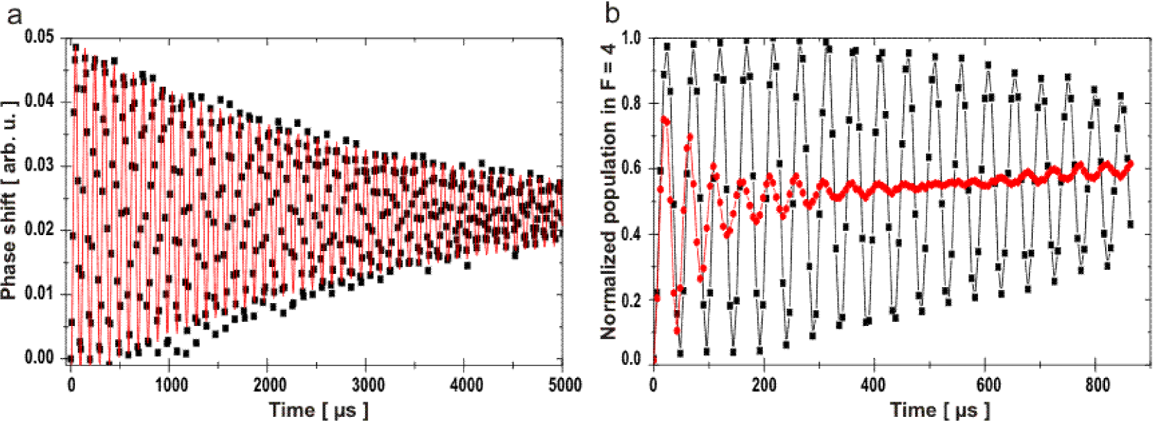
Figure 3: (a) Non–destructively probed Rabi oscillations. Each probe pulse contains about $10^{5}$ photons, is $0.2\,\mu$s long and the repetition period of the pulses is $10.3\,\mu$s. The data corresponds to an average of 10 runs of the experiment, each sampling the atoms $\sim 500$ times. The solid line corresponds to a fit, using a cosine function with exponential amplitude damping. (b) Changing the probe strength from $1.5\times 10^{5}$ photons per pulse (data indicated with $\blacksquare$) by a moderate factor of 4, a drastic change in the Rabi oscillation’s envelope occurs (data indicated by $\bullet$). The solid lines are to guide the eye, only.

oscillations recorded with the same probe pulse duration of $1.0\,\mu$s and the $7\,\mu$s repetition period but with different probe photon numbers. With $1.5\times 10^{5}$ photons per pulse we obtain a decay constant of $\tau=1.5$ ms, which reduces to $\tau=80\,\mu$s when the photon number per pulse is increased to $6.3\times 10^{5}$. This much faster decay cannot be explained just by the four times higher spontaneous excitation probability. Additionally, the trace corresponding to the higher probe power shows a clear revival of the oscillations at around $t=800\,\mu$s, and a change in the Rabi oscillation frequency is observable. In the following sections, we systematically analyze these effects and demonstrate that they can be well understood when taking the spatial inhomogeneity of the probe beam into account which causes a spatial distribution of the differential light shift between the clock states.

3 Inhomogeneous dephasing due to probe light shift

3.1 Bloch sphere picture and interpretation

We model the column density of the atomic sample on polar coordinates $(r,\phi)$ by $n(r)=n_{0}\exp(-2r^{2}/r_{0}^{2})$, where $n_{0}$ is the peak column density and $r_{0}$ characterizes the sample radius. The atomic sample interacts with a Gaussian laser beam propagating along the $z$-axis and focussed at the sample’s location. In the case when the axial size of the atomic sample is short compared to the Rayleigh range of the laser beam we can approximate the light intensity distribution within the interaction volume by $I(r)=I_{0}\exp(-2r^{2}/w_{0}^{2})$, where $I_{0}$ is the peak intensity and $w_{0}$ is the Gaussian beam waist.

The atoms in the sample are described by the two internal states $|3\rangle$ and $|4\rangle$ separated by an energy $E_{34}=\hbar\omega_{34}$ and on-resonance Rabi oscillations between the states can be induced by a drive field of angular frequency $\omega_{34}$ [26]. The laser beam is assumed to have a strong dispersive interaction with atoms in the $|4\rangle$ and negligible coupling to the $|3\rangle$ state. Hence, the population in the $|4\rangle$ state can be recorded as a phase shift of the laser beam. In turn, the dispersive interaction adds a differential light shift $\Delta E$ to $E_{34}$ (e.g.[29]).

The dynamics as a result of the combined action of continuously driving the $|3\rangle\leftrightarrow|4\rangle$ transition and acting on the sample with pulses of laser light at given instances of time is conveniently described in the Bloch sphere picture. A general superposition state $\cos\frac{\theta}{2}|3\rangle+e^{i\phi}\sin\frac{\theta}{2}|4\rangle$ is, up to a global phase, mapped onto the unit sphere at polar angle $\theta$ and azimuthal angle $\phi$ [30]. An ensemble state $\bf s$ is thus fully described by the two angles $\theta$ and $\phi$ or by its cartesian components ${\bf s}=s_{1}{\bf e}_{1}+s_{2}{\bf e}_{2}+s_{3}{\bf e}_{3}$. Pure states with all the atoms in $|3\rangle$ or $|4\rangle$ correspond to the Bloch vectors ${\bf s}=(0,0,-1)$ or ${\bf s}=(0,0,1)$, respectively. Under the influence of a resonant driving field of duration $t$, the initial atomic state $\bf s_{0}$ transforms according to

$${\bf s}(t)=\bar{\bar{U}}(t){\bf s}_{0}$$ (2)

$$\bar{\bar{U}}_{\mathrm{drive}}(t)=\left[\begin{array}[]{ccc}1&0&0\\ 0&\cos\Omega t&\sin\Omega t\\ 0&-\sin\Omega t&\cos\Omega t\\ \end{array}\right],$$ (3)

where $\Omega$ is the resonant Rabi frequency. Similarly, the dispersive interaction for a time $t$ is described by the evolution matrix

$$\bar{\bar{U}}_{\mathrm{probe}}(t)=\left[\begin{array}[]{ccc}\cos\chi t&\sin\chi t&0\\ -\sin\chi t&\cos\chi t&0\\ 0&0&1\\ \end{array}\right],$$ (4)

where $\chi=\Delta E/\hbar$. Since the problem is symmetric, the same rotation is induced by detuning the driving field from resonance by $\Delta E$ for a time $t$ or changing the phase of the driving field by $\chi t$. Finally, for the simultaneous action of the two effects we obtain the evolution matrix $\bar{\bar{U}}_{\mathrm{combined}}(t)$:

$$\left[\begin{array}[]{ccc}\frac{\Omega^{2}+\chi^{2}\cos\sqrt{\Omega^{2}+\chi^{2}}t}{{\Omega^{2}+\chi^{2}}}&\frac{\chi\sin\sqrt{\Omega^{2}+\chi^{2}}t}{\sqrt{\Omega^{2}+\chi^{2}}}&\frac{\Omega\chi(1-\cos\sqrt{\Omega^{2}+\chi^{2}}t)}{\Omega^{2}+\chi^{2}}\\ \frac{-\chi\sin\sqrt{\Omega^{2}+\chi^{2}}t}{\sqrt{\Omega^{2}+\chi^{2}}}&\cos\sqrt{\Omega^{2}+\chi^{2}}t&\frac{\Omega\sin\sqrt{\Omega^{2}+\chi^{2}}t}{\sqrt{\Omega^{2}+\chi^{2}}}\\ \frac{\Omega\chi(1-\cos\sqrt{\Omega^{2}+\chi^{2}}t)}{\Omega^{2}+\chi^{2}}&\frac{-\Omega\sin\sqrt{\Omega^{2}+\chi^{2}}t}{\sqrt{\Omega^{2}+\chi^{2}}}&\frac{\chi^{2}+\Omega^{2}\cos\sqrt{\Omega^{2}+\chi^{2}}t}{{\Omega^{2}+\chi^{2}}}\\ \end{array}\right]$$ (5)

The evolution of an initial Bloch vector $\bf s_{0}$ can now be propagated by multiplying the corresponding matrices, e.g. (3) and (5) in succession to get an overall transfer matrix $T(\chi,t)$. In the experiment, we only have direct access to the $3$–projection of the Bloch vector.

Due to the Gaussian intensity profile of the laser beam, we get a position dependent light shift and $\chi$ will vary radially as $\propto I(r)$. Moreover, in the detection of the $3$-projection of $\bf s$, the Gaussian intensity dependence of the laser beam in conjunction with the Gaussian column density of the atomic sample gives rise to a signal

$$S_{\phi}(t) \propto \int_{0}^{\infty}[T(\chi(r),t){\bf s}]_{3}n(r)I(r)rdr$$ (6)

$$\propto \int_{0}^{\infty}[T(\chi(r),t){\bf s}]_{3}n_{0}I_{0}e^{-2(\frac{r}{r_{0}})^{2}}e^{-2(\frac{r}{w_{0}})^{2}}rdr$$

$$\propto \int_{0}^{\chi_{0}}[T(\chi,t){\bf s}]_{3}\chi^{(\frac{w_{0}}{r_{0}})^{2}}d\chi,$$

where $\chi_{0}=\chi(r=0)$ corresponds to the maximum light shift at the center of the Gaussian beam. Hence, for a given ratio between $r_{0}$ and $w_{0}$ the net measured Bloch vector results from infinitesimal contributions from atoms with light shifts $\chi=[0...\chi_{0}]$ carrying a weight $\chi^{(\frac{w_{0}}{r_{0}})^{2}}$. In Fig. 4c we plot the weighting factor for a few values of the ratio $k=w_{0}/r_{0}$. As would be expected, the atoms contributing to the net Bloch vector have undergone practically the same light shift close to the maximum $\chi_{0}$ if the laser beam waist is much larger than the atomic sample radius $w_{0}\gg r_{0}$. At the other extreme $w_{0}\ll r_{0}$, our detected signal will have a uniform contribution from light shifts in the interval $[0...\chi_{0}]$.

3.2 Application to Rabi oscillations

3.2.1 Expected behavior from the theoretical model

Let us first consider the theoretical model for the case of alternating microwave driving field and probe pulses. If we neglect the inhomogeneity of the induced light shift, each single probe pulse will cause the tip of the Bloch vector to rotate around the $3$–axis according to the transformation matrix (4) by an angle $\chi t$, proportional to the number of photons of the probe pulse. Alternating microwave pulses, rotating around the $1$–axis according to matrix (3), and probe pulses, we expect a step–like evolution as shown in Fig. 4a.

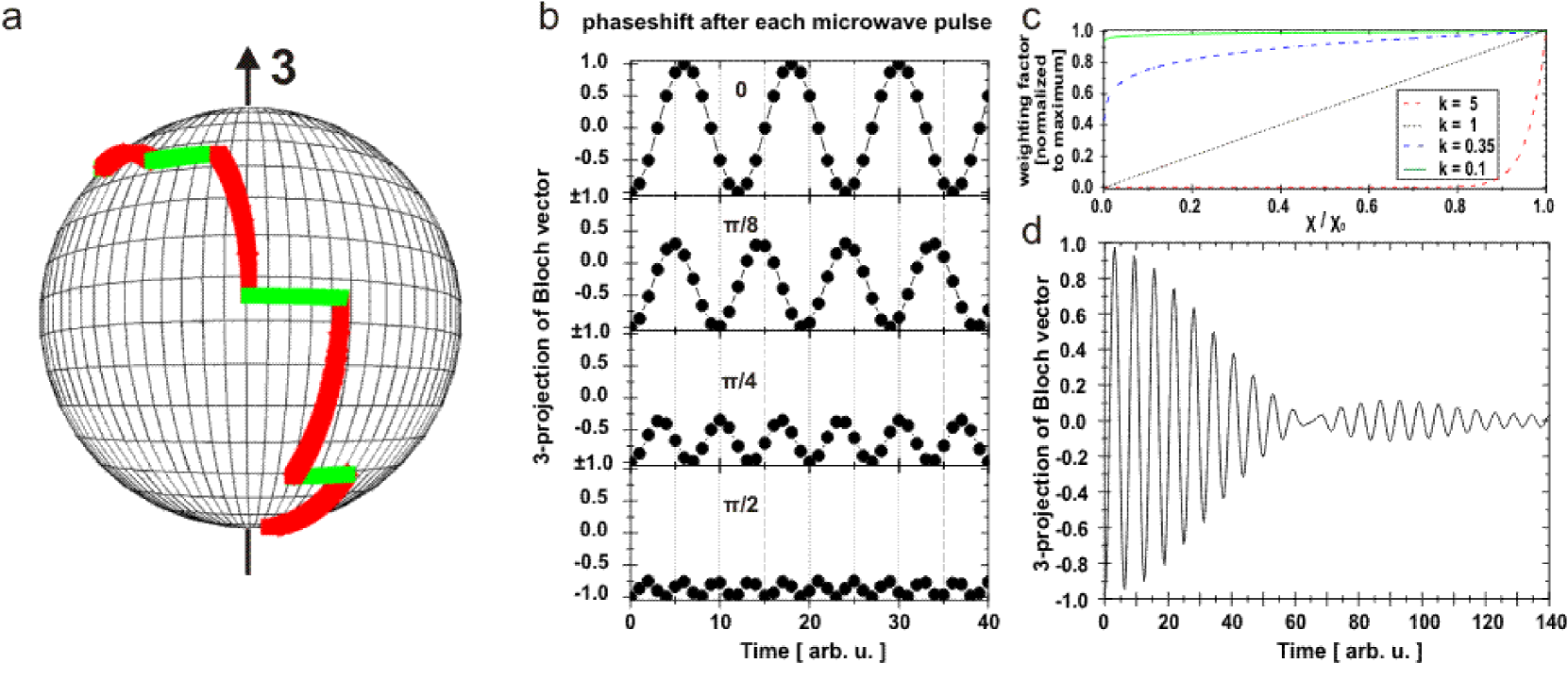
Figure 4: (a) State evolution on the Bloch sphere with alternating microwave pulses, each pulse shifting by $\pi/4$ around the $1$–axis, and probe pulses, each causing a homogeneous shift of $\pi/9$ around the $3$–axis. (b) 3– projection of the Bloch vector for different homogeneous light shifts, applied discretely in between separated $\pi/6$ microwave pulses. (c) Weighting factor of the oscillations with different frequency due to the inhomogeneity of the probe beam and the sample. The factor is plotted for different ratios $k$ of the probe beam waist $\omega_{0}$ to the sample size $r_{0}$, and normalized to its maximum value. For large ratios $k\gg 1$, an almost homogeneous shift is induced, for small ratios $k\ll 1$ the distribution is flat. (d) Rabi–oscillations resulting from inhomogeneous light shift distribution across the probe area.

In figure 4b, we show the expected measurement result for each probe pulse when changing the photon number or the rotation angle $\chi t$ induced per probe pulse. As can be seen, the discretely induced transition frequency change $\Delta E=\hbar\chi$ at discrete times, resulting from the differential light shift between the clock states, leads to a higher effective Rabi frequency $\Omega^{\prime}=\sqrt{\Omega^{2}+\overline{\Delta E}^{2}}$. Here $\overline{\Delta E}=\frac{1}{2\pi}\int\Delta E(t)dt$ is the time averaged frequency change. This effect is very similar to the Rabi frequency change one observes when the transition frequency is continuously shifted relative to the driving field by $\Delta E$ e.g. due to off–resonant driving [30] or a homogeneous light shift across the sample [3]. Introducing a light–shift at discrete intervals changes the observed Rabi frequency stepwise during the single period, however, after each period $T=\frac{2\pi}{\Omega}$ the effect is the same as if the transition frequency had been changed by a mean value $\overline{\Delta E}$ during the whole period. In the experiment, a continuous distribution of light shifts $\chi=[0\dots\chi_{0}]$ is present and thus oscillations of different frequencies, weighted in amplitude with the density distribution of the sample across the probe beam, interfere. The resulting oscillations are shown in Fig. 4d for a probe size to sample ratio $k=0.35$ and a maximum shift of $\chi_{0}=0.3$ rad per pulse.

3.2.2 Experimental results

To study the perturbing effects of the inhomogeneous atom-probe interaction systematically, we alternate microwave and probe pulses and record data sets for different probe powers. In Fig. 5a we show a collection of data together with fits of the theoretical model from equation (6). In the fitting model, we have allowed for a small number of spontaneous scattering events, pumping atoms into the $6S_{1/2}(F=4,m_{F}\neq 0)$ states and homogeneous dephasing mechanisms like magnetic background fluctuations, microwave driving field inhomogeneities or cloud temperature effects [31].

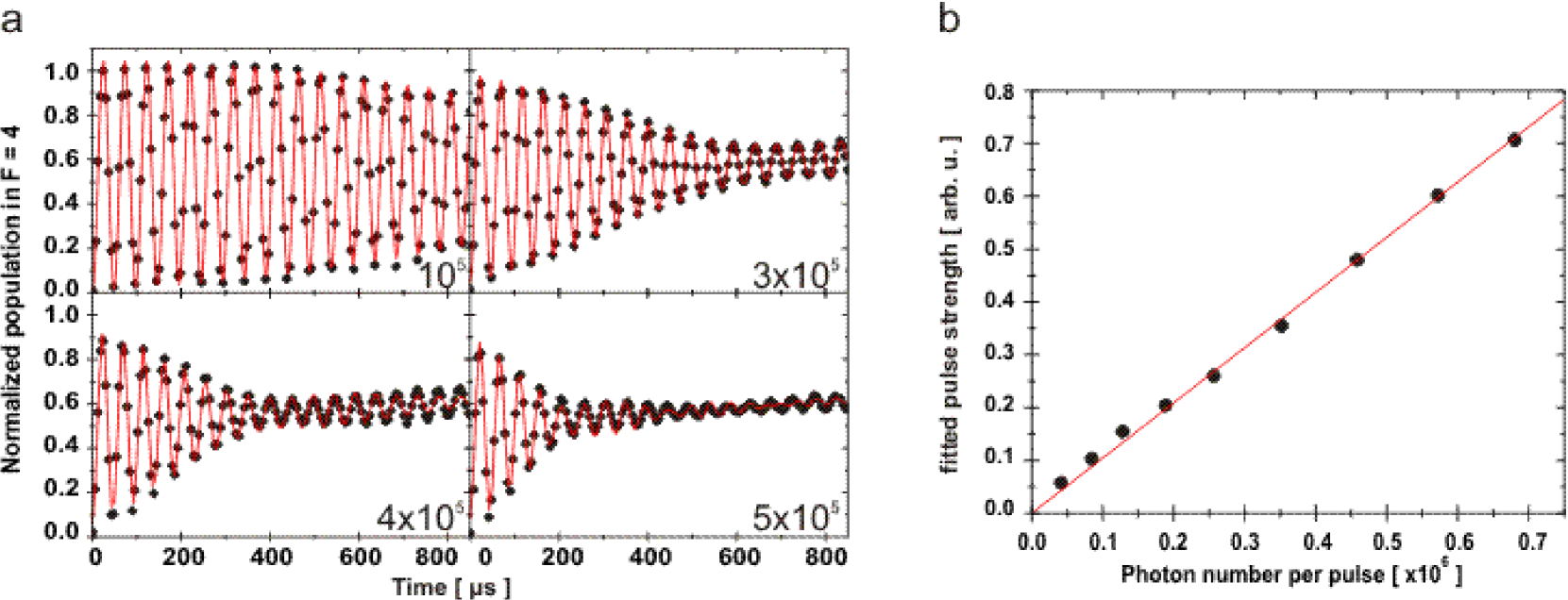
Figure 5: (a) Non–destructively probed Rabi oscillations. The photon number per probe pulse is given in the lower right corner of each graph. The solid line represents a fit to the data with the model discussed in the text. (b) Comparison of the photon number per pulse as measured in the experiment to the pulse strength returned from the fitting routine. The scaling is well described by a linear function through the origin.

The data is remarkably well described by the simple model. In particular, the envelope together with the revival of the oscillations is very well reproduced. The fitting routine returns a parameter $\propto\chi_{0}$, the maximum phase spread cause by the light shift, which is expected to be directly proportional to the photon number in the light–shifting pulses. The value is shown in Fig. 5b as function of the applied photon number, confirming the validity of our model within the given parameter range.

3.3 Ramsey spectroscopy

A more direct measurement of the phase shift induced by the probing can be obtained with Ramsey spectroscopy [21].

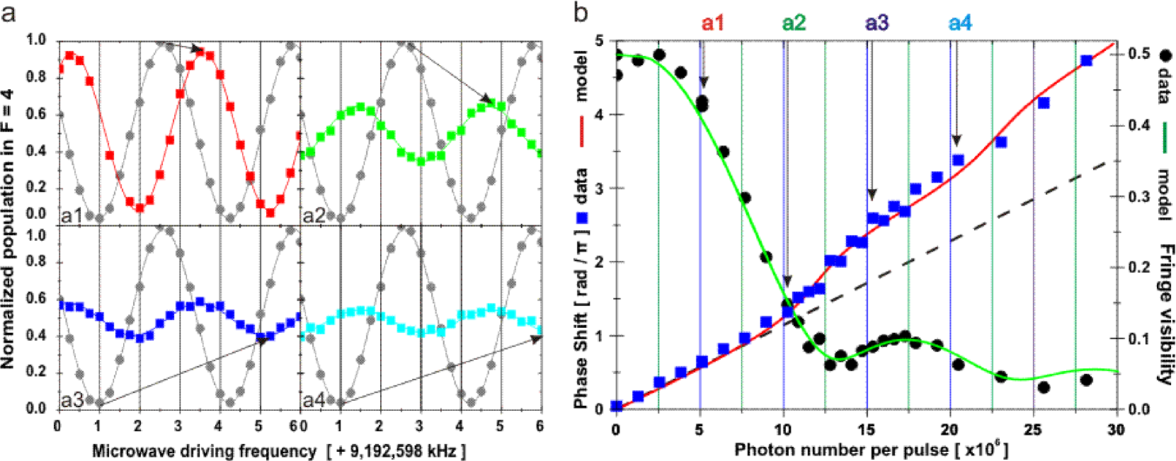
Figure 6: (a) Ramsey fringes, discrete points represent experimental data, the solid lines are cosine fits to the data. The data indicated with $\bullet$ represents the reference trace where no light shifting pulse has been applied to the superposition state during the Ramsey sequence. From (a1)–(a4), the probe pulse photon number has been doubled in each step, starting with $2.6\times 10^{6}$. (b) Normalized phase shift and fringe amplitude of Ramsey fringes, extracted from data similar to (a1)–(a4). The solid lines represent the theory curves and follow the experimental data remarkably well. The dashed line in the phase shift data corresponds to the linear dependence expected for a homogeneous system.

Briefly, the basic principle is as follows: Beginning from an initial state, where all atoms reside in $|3\rangle$, a $\pi/2$–pulse brings the ensemble into a superposition state $\frac{1}{\sqrt{2}}(|3\rangle+|4\rangle)$. The quantum state then evolves freely, in our case for a time of $300\,\mu$s. The population measured in $|4\rangle$ after a second $\pi/2$–pulse depends on the relative phase $\phi$ between the two atomic states $\frac{1}{\sqrt{2}}(|3\rangle+e^{i\phi}|4\rangle)$ acquired during the free evolution. For $\phi\mbox{ mod }2\pi=0$ we end up at $|4\rangle$, $\phi\mbox{ mod }2\pi=\pi$ yields $|3\rangle$ and $\phi\mbox{ mod }2\pi=(\pi/2,3\pi/2)$ yields $\frac{1}{\sqrt{2}}(|3\rangle\pm|4\rangle)$. As discussed in section 3.1, such a phase shift can be induced by shifting the transition out of resonance, e.g. by applying a probe pulse, or by detuning the driving field from resonance. The latter yields well–known Ramsey fringes [22], shown as reference in Fig. 6a. Again, the population observed in $|4\rangle$ is normalized to the number of atoms. When we, in addition, apply light shifting pulses (simply by using the probe beam for this purpose) while the atomic state evolves freely, the differential light shift adds a phase shift distribution proportional to the number of photons interacting with the atoms. Accordingly, the Ramsey fringes will be shifted in frequency space, which can be clearly seen in graphs (a1)–(a4) of Fig. 6a. By normalizing the frequency shift to the period of the Ramsey fringes, we can directly extract the mean phase shift angle caused by the probe. In a homogeneous system as studied by Featonby et al. [21], the Ramsey fringe position shifts proportionally to the photon number of the probe pulse. In the inhomogeneous situation we are considering, the spatial profile of the light pulse will create a phase shift distribution along the equator as discussed in section 3.1. We can therefore no longer expect the shift to be exactly proportional to the probe pulse strength, since states gaining the same phase angle $\phi=(\chi t\ \mbox{ mod }\ 2\pi)$ are equivalent in a Ramsey experiment. The phase distribution of the ensemble also acts to wash out the Ramsey fringe visibility, since the externally introduced distribution is basically a standard dephasing mechanism.
In Fig. 6b the normalized phase shift and amplitude of the fringes, extracted from the Ramsey spectroscopy measurements are shown. One can see a clear deviation from a linear scaling when the accumulated phase shift exceeds $2\pi$. The Ramsey fringe amplitude also shows the expected revival when the phase distribution starts to overlap above $2\pi$ and Bloch vector components with the same phase modulo $2\pi$ interfere constructively. The graph also contains the theoretical predictions from the model given above and a good correspondence is observed.

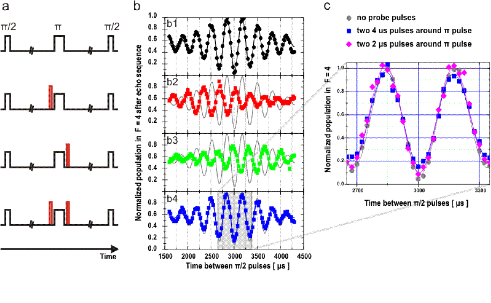
Figure 7: (a) Pulse sequence for spin echo measurements. The black lines correspond to the microwave pulses and the red lines indicate the placement of the probe pulses. (b) Spin echo signal observed according to the corresponding pulse sequences to the left. The fit to the plain spin echo trace (b1) is kept for reference in graphs (b2)–b(4). Additional probe pulses, duration $4\,\mu$s, containing $\sim 10^{6}$ photons, during the echo sequence shift the echo signal in time space (b2)–(b3), corresponding to the mean phase shift imprinted onto the ensemble. Distributing the probe pulse around the re–phasing microwave pulse, amplitude and phase of the echo signal are regained. The solid lines represent fits to the data, assuming a Gaussian envelope of the echo signal. (c) A zoom into the central part of the echo signal shows that the ensemble can be fully re–phased when the probe pulses are distributed symmetrically around the microwave echo pulse. The slight reduction of the fringe contrast when doubling the photon number is due to photon scattering

4 Sample re–phasing with spin echo

The inhomogeneous phase spread of the ensemble after a measurement poses a serious problem for spectroscopy, squeezing, and quantum information applications and challenges the non–destructive nature of the measurement. Obviously, for probe pulses with large photon numbers, the atomic state evolution is dominated by the effect of the probing. Using such a strongly perturbing probe beam, e.g. to predict the quantum state of the ensemble, creates a state whose phase is distributed around the equator of the Bloch sphere. When interrogating an ensemble with $N$ atoms, one can still gain information about the z–projection of the state to better than $1/\sqrt{N}$ — the standard quantum limit — and thus achieve spin squeezing, but due to the large phase distribution, the remaining state will be of little use for spectroscopic applications. It is, however, possible to re-phase the ensemble after a dispersive measurement by applying spin echo techniques [32]. To achieve re-phasing, we invert the time evolution of the spreading by adding a microwave $\pi$–pulse between the two Ramsey $\pi/2$–pulses. To again study the effect of the differential light shift distribution when probing the sample, light pulses are symmetrically distributed around this refocusing $\pi$–pulse. The pulse sequence for these echo measurements is illustrated in Fig. 7a. After the pulse sequence, we measure the population in $|4\rangle$ with further probe pulses and normalize to the total number of atoms.
The plain spin echo sequence, taking care of dephasing e.g. caused by the trapping laser, shows a close to perfect refocussing of the sample at the expected time as shown in Fig. 7b,(b1). When applying a single probe pulse before or after the echo pulse, the echo fringe is shifted in time according to the induced mean phase shift by the probe pulses, figure 7b,(b2)–(b3). As with the Ramsey fringes in Fig. 6a, the inhomogeneity of the light shift reduces the echo fringe visibility drastically. If we, however, apply light pulses symmetrically around the spin echo pulse, Fig. 7b,(b4) shows that we regain the unshifted echo fringe almost perfectly. In graph 7c we zoom in on the central Ramsey fringe to back up this claim. The graph also confirms that the measurements are indeed not limited by off–resonant photon scattering. When the ensemble is in a superposition state, both inelastic Raman and elastic Rayleigh scattering would lead to complete decoherence of the excited atoms and reduce the fringe contrast. However, as can be seen in the graph 7c, the fringe contrast is, not reduced appreciably. The influence of photon scattering is slightly visible when comparing the fringe amplitudes of echo signals with different probe pulse powers. From the magnitude of the change, however, we conclude that they are of minor consideration here. In addition, the data confirms that other dephasing mechanisms e.g. due to the non–zero temperature of the cloud or magnetic background fluctuations are also of minor importance.

5 Discussion

We use a dispersive phase shift measurement to non– destructively probe the populations of the clock states in a cold Cs ensemble when subjected to near resonant microwave pulses. The strong dependence of the Rabi oscillation envelope on the probe pulse photon numbers — causing a differential light shift between the clock states and thus adding a relative phase between the clock states — can only be explained by the inhomogeneity of the light–atom interaction, which is intrinsic to the experimental setup. With the introduced theoretical model, the experimental data can be convincingly explained. To quantify the dephasing of the atomic ensemble induced by the probing, Ramsey spectroscopy in the frequency domain is used, and both the scaling of the phase shift of the Ramsey fringes and the scaling of their amplitude with applied photon number in the probe pulses can be explained by the same model. Finally, the application of spin echo techniques allow us to re–phase the atomic sample.
We note that for the range of probe intensities applied in the experiments presented in the current paper, the effect of spontaneous photon scattering from the probe pulses can be neglected. Furthermore, other decoherence effects e.g. due to finite temperature of the ensemble or magnetic field fluctuations can be disregarded on the given timescales. However, to achieve considerable spin squeezing in the presented experimental configuration, considerably higher probe powers implying about 20 % spontaneous scattering probability are necessary [10]. When other decoherence effects are under control, spin echo techniques can be used to calibrate these effects as well [33].

The differential light shift between the clock states due to the probe light is, of course, caused by the choice of the probe detuning. By choosing a “magic” frequency for the probe, where both clock levels are shifted by the same amount, the induced dephasing of the two levels can be minimized and in the ideal case, canceled [3]. Since the presented single frequency probing scheme is only sensitive to the scalar polarizability of the atoms, the magic frequencies coincide with the probe detunings where the interferometer phase shift is insensitive to the population number difference. Single frequency measurements are thus not suited to eliminate the perturbation of the atomic levels. The problem can be circumvented by adding a second probe frequency or invoking the tensor polarizability in off–resonant polarization measurements [34].

This work was funded by the Danish National Research Foundation, as well as the EU grants QAP and COVAQUIAL. N.K. acknowledges the support of the Danish National Research Council through a Steno Fellowship. We would like to thank Jörg Helge Müller for stimulating discussions.

References

- [1] L.E. Sadler, J.M. Higbie, S.R. Leslie, M. Vengalattore, D. Stamper-Kurn, Nature 443, 312 (2006)
- [2] P.G. Petrov, D. Oblak, C.L. Garrido Alzar, N. Kjærgaard, E.S. Polzik, Phys. Rev. A 75, 033803 (2007)
- [3] S. Chaudhury, G.A. Smith, K. Schulz, P.S. Jessen, Phys. Rev. Lett. 96, 043001 (2006)
- [4] K. Usami, M. Kozuma, Phys. Rev. Lett. 99, 140404 (2007)
- [5] P.J. Windpassinger, D. Oblak, P.G. Petrov, M. Kubasik, M. Saffman, C.L. Garrido Alzar, J. Appel, J. Müller, N. Kjærgaard, E.S. Polzik, Phys. Rev. Lett. 100, at press (Preprint arXiv:0801.4126) (2008)
- [6] A. Kuzmich, N.P. Bigelow, L. Mandel, EuroPhys. Lett. 42, 481 (1998)
- [7] B. Julsgaard, A. Kozhekin, E.S. Polzik, Nature 413, 400 (2001)
- [8] J. Geremia, J. Stockton, H. Mabuchi, Science 304, 270 (2004)
- [9] J. Sherson, B. Julsgaard, E. Polzik, Adv. At. Mol. Opt. Phys. 54 (2006)
- [10] K. Hammerer, K. Mølmer, E.S. Polzik, J.I. Cirac, Phys. Rev. A 70, 044304 (2004)
- [11] B. Julsgaard, J. Sherson, J.I. Cirac, J. Fiurasek, E.S. Polzik, Nature 432, 482 (2004)
- [12] J.F. Sherson, H. Krauter, R.K. Olsson, B. Julsgaard, K. Hammerer, I. Cirac, E.S. Polzik, Nature 443, 557 (2006)
- [13] G. Santarelli, P. Laurent, P. Lemonde, A. Clairon, A.G. Mann, S. Chang, A.N. Luiten, C. Salomon, Phys. Rev. Lett. 82, 4619 (1999)
- [14] D.J. Wineland, J.J. Bollinger, W.M. Itano, F.L. Moore, D.J. Heinzen, Phys. Rev. A 46, R6797 (1992)
- [15] D.J. Wineland, J.J. Bollinger, W.M. Itano, D.J. Heinzen, Phys. Rev. A 50, 67 (1994)
- [16] D. Oblak, P.G. Petrov, C.L. Garrido Alzar, W. Tittel, A.K. Vershovski, J.K. Mikkelsen, J.L. Sørensen, E.S. Polzik, Phys. Rev. A 71, 043807 (2005)
- [17] D. Meiser, J. Ye, M.J. Holland, Preprint arXiv:0707.3834
- [18] M. Takamoto, F.L. Hong, R. Higashi, H. Katori, Nature 435, 321 (2005)
- [19] R. Le Targat, X. Baillard, M. Fouché, A. Brusch, O. Tcherbakoff, G.D. Rovera, P. Lemonde, Phys. Rev. Lett. 97, 130801 (2006)
- [20] A.D. Ludlow, M.M. Boyd, T. Zelevinsky, S. Foreman, S. M.and Blatt, M. Notcutt, T. Ido, J. Ye, Phys. Rev. Lett. 96, 033003 (2006)
- [21] P.D. Featonby, C.L. Webb, G.S. Summy, C.J. Foot, K. Burnett, J. Phys. B 31, 375 (1998)
- [22] J. Vanier, C. Audoin, The Quantum Physics of Atomic Frequency Standards (Adam Hilger, 1989)
- [23] R. Grimm, M. Weidemüller, Y.B. Ovchinnikov, Adv. At. Mol. Opt. Phys. 42, 95 (2000)
- [24] G. Avila, V. Giordano, V. Candelier, E. Declercq, G. Theobald, P. Cerez, Phys. Rev. A 36, 3719 (1987)
- [25] P. Tremblay, C. Jacques, Phys. Rev. A 41, 4989 (1990)
- [26] C. Cohen-Tannoudji, B. Diu, F. Laloë, Quantum Mechanics (Wiley, New York, 1977)
- [27] R. Loudon, The Quantum Theory of Light (Oxford University Press, 1973)
- [28] R. Ozeri, C. Langer, J.D. Jost, B. DeMarco, A. Ben-Kish, B.R. Blakestad, J. Britton, J. Chiaverini, W.M. Itano, D.B. Hume et al., Phys. Rev. Lett. 95, 030403 (2005)
- [29] H. Metcalf, P. van der Straten, Laser Cooling and Trapping (Springer, Berlin, 1999)
- [30] L. Allen, J.H. Eberly, Optical Resonance and Two-Level Atoms (Dover, New York, 1987)
- [31] S. Kuhr, W. Alt, D. Schrader, I. Dotsenko, Y. Miroshnychenko, A. Rauschenbeutel, D. Meschede, Phys. Rev. A 72, 023406 (2005)
- [32] M.F. Andersen, A. Kaplan, N. Davidson, Phys. Rev. Lett. 90, 023001 (2003)
- [33] D. Oblak, et al., in preparation (2008)
- [34] M. Saffman, et al., in preparation (2007)