The Tidal Streams of Disrupting Subhaloes in Cosmological Dark Matter Haloes

Abstract

We present a detailed analysis of the properties of tidally stripped material from disrupting substructure haloes or subhaloes in a sample of high resolution cosmological $N$-body host haloes ranging from galaxy- to cluster-mass scales. We focus on devising methods to recover the infall mass and infall eccentricity of subhaloes from the properties of their tidally stripped material (i.e. tidal streams). Our analysis reveals that there is a relation between the scatter of stream particles about the best-fit debris plane and the infall mass of the progenitor subhalo. This allows us to reconstruct the infall mass from the spread of its tidal debris in space. We also find that the spread in radial velocities of the debris material (as measured by an observer located at the centre of the host) correlates with the infall eccentricity of the subhalo, which allows us to reconstruct its orbital parameters. We devise an automated method to identify leading and trailing arms that can, in principle at least, be applied to observations of stellar streams from satellite galaxies. This method is based on the energy distribution of material in the tidal stream. Using this method, we show that the mass associated with leading and trailing arms differ. While our analysis indicates that tidal streams can be used to recover certain properties of their progenitor subhaloes (and consequently satellites), we do not find strong correlations between host halo properties and stream properties. This likely reflects the complicated relationship between the stream and the host, which in a cosmological context is characterised by a complex mass accretion history, an asymmetric mass distribution and the abundance of substructure. Finally, we confirm that the so-called “backsplash” subhalo population is present not only in galaxy cluster haloes but also in galaxy haloes. The orbits of backsplash subhaloes brought them inside the virial radius of their host at some earlier time, but they now reside in its outskirts at the present-day, beyond the virial radius. Both backsplash and bound subhaloes experience similar mass loss, but the contribution of the backsplash subhaloes to the overall tidal debris field is negligible.

1 Introduction

The currently favoured model for cosmological structure formation is the $\Lambda$CDM model. This model assumes that we live in a spatially flat Universe whose matter content is dominated by non-baryonic Cold Dark Matter (CDM) and whose present-day expansion rate is accelerating, driven by Dark Energy ($\Lambda$). In the context of this model, the formation and evolution of cosmic structure proceeds in a “bottom-up” or hierarchical manner. Low mass gravitationally bound structures merge to form progressively more massive structures, and it is through such a merging hierarchy that galaxies, groups and clusters form (e.g. Davis et al. 1985; Springel et al. 2006).

The tidal disruption of satellite galaxies around our Galaxy and others is characteristic of the hierarchical merging scenario. As a satellite galaxy orbits within the gravitational potential of its more massive host, it is subject to a tidal field that may vary in both space and time. The gravitational force acting on the satellite strips a stream of tidal debris from it, and in some cases tidal forces may be sufficient to lead to the complete disruption of the system. This tidal debris tends to form two distinct arms – a leading arm ahead of the satellite and a trailing arm following the satellite.

The process by which a satellite galaxy suffers mass loss and the subsequent formation of a stream of tidal debris (hereafter referred to as a tidal stream) has been studied extensively using numerical simulations (e.g. Johnston 1998; Ibata et al. 2001; Helmi 2004). A number of these studies have followed the orbital evolution of an individual satellite galaxy with a known mass profile, realised with many particles, in a static analytic and non-cosmological host potential (e.g. Johnston 1998; Ibata et al. 2001; Helmi 2004, and many others). This approach allows for well-defined test cases to be investigated and for a systematic survey of orbital and structural parameters to be carried out. For example, Helmi (2004) showed that the width of the tidal debris in the plane perpendicular to its orbit increases when the host halo potential is flattened rather than spherical.

In this regard, it is important to note that stream properties are sensitive to both the internal properties of its progenitor satellite and the details of the orbit that it follows. For example, we expect the length and width of a stream to tightly correlate with the age of the stream and the mass/internal velocity dispersion of its progenitor (e.g. Johnston et al. 1996; Johnston 1998; Johnston et al. 2001; Peñarrubia et al. 2006). Understanding what role the progenitor satellite and its orbit plays in shaping stream properties is therefore vital if we wish to use streams to address more fundamental problems, such as the nature of the dark matter.

While previous studies have provided important insights into the formation and evolution of tidal streams and their dependence on the properties of both satellites and host dark matter haloes, none have considered tidal streams in cosmological host haloes. Cosmological haloes have complex mass accretion histories and mass distributions that can at best be crudely approximated by fitting formulae, and the interplay between a halo’s asphericity, its clumpiness, and how its mass grows in time may be non-trivial. How this complexity may affect the results of previous studies, which were based on analytic potentials and approximations to halo growth, is difficult to say. For example, interactions between the stream and substructures lead to the dynamical heating, causing an increase in internal velocity dispersion and a subsequent broadening of the stream (Moore et al. 1999; Ibata et al. 2002; Johnston et al. 2002). Therefore, while studying tidal streams in cosmological haloes is a challenging problem, such an approach is necessary if our results are to reflect the complexity of nature (assuming the validity of the $\Lambda$CDM model, of course!).

This paper is the first of in a series that will examine the formation and evolution of tidal streams in cosmological dark matter haloes, and determine how the properties of these tidal streams depend on the properties of the satellite galaxies from which they originate and on the host dark matter haloes in which they orbit. We use high resolution cosmological simulations of individual galaxy- and cluster-mass dark matter haloes – the host haloes – that allow us to track in detail the evolution of a large population of their substructures or satellite galaxies over multiple orbits. We seek to answer the questions we consider to be key to the study of tidal streams;

• Can observations of tidal streams be used to infer the properties of their parent satellite?

• Can tidal streams reveal properties of the underlying dark matter distribution of the host halo?

The present paper primarily focuses on the first question and can be summarised as follows. In Section 2 we describe the fully self-consistent cosmological simulations of structure formation in a $\Lambda$CDM universe that we have used in our study. The suite of host haloes (consisting of eight cluster and one Milky Way sized dark matter halo) are presented in Section 3. In Section 4 we shift attention to the formation and evolution of debris fields. In this regard, Section 4 deals with mass loss from subhaloes and the contribution of so-called “backsplash” satellites. These subhaloes are found outside the virial region of the host at the present day, but their orbits took them inside the virial radius at earlier times. We show that they exist not only in cluster-sized haloes as found by e.g. Gill et al. (2005) and Moore et al. (2004), but also in our galactic halo. In Section 5 we examine how well satellite properties such as its original mass and the eccentricity of its orbit can be reproduced using the whole debris field of the corresponding satellite. Furthermore, we present in Section 6 a method to distinguish between trailing and leading arms in an automated fashion and we investigate properties of the streams such as their mass, shape and velocity dispersion. We pay particular interest to the energy distribution of debris, since it can be used to distinguish between leading and trailing arm observationally. Finally, we summarise our results in Section 7 and comment on their significance in the context of future papers, which will try to establish the missing link between the properties of tidal streams and the host haloes only briefly touched upon in this study.

2 Simulations & Analysis Methods

2.1 The Simulations

Our analysis is based on a set of nine high-resolution cosmological $N$-body simulations that were used in the study of Warnick & Knebe (2006). These simulations focus on the formation and evolution of a sample of galaxy- and cluster-mass dark matter haloes forming in a spatially flat $\Lambda$CDM cosmology with $\Omega_{0}$=0.3, $\Omega_{\Lambda}$=0.7, $\Omega_{b}$=0.04, $h$ = 0.7, and $\sigma_{8}$ = 0.9. Each halo contains at least $10^{6}$ particles at $z$=0 and each simulation was run with an effective spatial resolution of $\leq 0.01R_{\rm vir}$.

Eight of the haloes – the cluster-mass systems, C1-C8 – were simulated using the publicly available adaptive mesh refinement code MLAPM Knebe et al. (2001). We first created a set of four independent initial conditions at redshift $z=45$ in a standard $\Lambda$CDM cosmology ($\Omega_{0}=0.3,\Omega_{\lambda}=0.7,\Omega_{b}=0.04,h=0.7,\sigma_{8}=0.9$). $512^{3}$ particles were placed in a box of side length 64$h^{-1}{\ }{\rm Mpc}$ giving a mass resolution of $m_{p}=1.6\times 10^{8}$$h^{-1}{\ }{\rm M_{\odot}}$. For each of these initial conditions we iteratively collapsed eight adjacent particles to one particle reducing our particle number to 128³ particles. These lower mass resolution initial conditions were then evolved until $z=0$. At $z=0$, eight clusters (labeled C1-C8) from our simulation suite were selected, with masses in the range 1–3$\times 10^{14}$$h^{-1}{\ }{\rm M_{\odot}}$. Then, as described by Tormen (1997), for each cluster the particles within five times the virial radius were tracked back to their Lagrangian positions at the initial redshift ($z=45$). Those particles were then regenerated to their original mass resolution and positions, with the next layer of surrounding large particles regenerated only to one level (i.e. 8 times the original mass resolution), and the remaining particles were left 64 times more massive than the particles resident with the host cluster. This conservative criterion was selected in order to minimise contamination of the final high-resolution haloes with massive particles.

The ninth (re-)simulation was performed using the same (technical) approach but with the ART code (Kravtsov et al. 1997). Moreover, this particular run (labeled G1) describes the formation of a Milky Way type dark matter halo in a box of side 20$h^{-1}{\ }{\rm Mpc}$. It is the same simulation as “Box20” presented in Prada et al. (2006) and for more details we refer the reader to that study. The final object consists of about two million particles at a mass resolution of $6\times 10^{5}$$h^{-1}{\ }{\rm M_{\odot}}$ per particle and a spatial force resolution of 0.15$h^{-1}{\ }{\rm kpc}$ has been reached. All nine simulations have the required temporal resolution (i.e. $\Delta t\approx$ 200 Myrs for the clusters and $\Delta t\approx$ 20 Myrs for the galactic halo, respectively) to accurately follow the formation and evolution of subhaloes within their respective hosts and hence are well suited for the study presented here. The high mass and force resolution of our simulations is sufficient to resolve an abundance of substructure (the “satellites” in our study) within the virial radius of each host.

The physical properties of the haloes (based upon the halo finding technique explained below) are summarised in Table 1 alongside some additional indicators quantifying the mass assembly histories (cf. Section 3).

2.2 Halo Finding

Both the haloes and their subhaloes are identified using AHF, an MPI parallelised modification of the MHF algorithm presented in Gill et al. (2004). AHF utilises the adaptive grid hierarchy of MLAPM to locate haloes (subhaloes) as peaks in an adaptively smoothed density field. Local potential minima are computed for each peak and the set of particles that are gravitationally bound to the peak are returned. If the peak contains in excess of 20 particles, then it is considered a halo (subhalo) and retained for further analysis.

For each halo (subhalo) we calculate a suite of canonical properties from particles within the virial/truncation radius. We define the virial radius $R_{\rm vir}$ as the point at which the density profile (measured in terms of the cosmological background density $\rho_{b}$) drops below the virial overdensity $\Delta_{\rm vir}$, i.e. $M(<R_{\rm vir})/(4\pi R_{\rm vir}^{3}/3)=\Delta_{\rm vir}\rho_{b}$. Following convention, we assume the cosmology- and redshift-dependent definition of $\Delta_{\rm vir}$; for a distinct (i.e. host) halo in a $\Lambda$CDM cosmology with the cosmological parameters that we have adopted, $\Delta_{\rm vir}=340$ at $z=0$. This prescription is not appropriate for subhaloes in the dense environs of their host halo, where the local density exceeds $\Delta_{\rm vir}\rho_{b}$, and so the density profile will show a characteristic upturn at a radius $R\mathrel{\hbox{\hbox to0.0pt{\hbox{\lower 4.0pt\hbox{$\sim$}}\hss}\hbox{$<$}}}R_{\rm vir}$. In this case we use the radius at which the density profile shows this upturn to define the truncation radius for the subhalo. Further details of this approach can be found in Gill et al. (2004).

2.3 Subhalo Tracking

In the present study we are primarily interested in the temporal evolution and disruption of subhaloes and hence a simple halo finder will not suffice. Therefore we base our analysis on the halo tracking method outlined in Gill et al. (2004). At the formation time of the host halo we identify all subhaloes in its immediate environment using AHF and track their subsequent evolution using the set of particles identified at the initial time. Using the 25 innermost particles at time $t_{1}$ we calculate the new subhalo centre at the subsequent time $t_{2}$. We then check which of the initial set of particles remain bound to the subhalo; all unbound particles constitute “debris”. Particles are unbound if their speed exceeds the escape velocity by a factor of 1.5. This tolerance factor is introduced to allow for any inaccuracy arising from the assumption of spherical symmetry or uncertainties in the extent of the subhalo. All particles, bound as well as unbound ones, are tracked forward to the present day, which allows us to look at the field of debris particles for each subhalo.

The tracker does not take into account accretion of mass, and so we may slightly underestimate subhalo masses. However, it is very unlikely that subhaloes will accrete material as they orbit within the host; rather, they will suffer continuous mass loss. In contrast to a simple halo finder, the tracker is able to detect “flickering” subhaloes that temporarily disappear in the dense inner regions of the host (e.g. Power & Knebe 2007). The tracker is in the exceptional position of knowing that there should be a subhalo and thus can track it as it orbits within the densest innermost parts of the host (see Gill et al. 2004).

However, there is one draw-back with this otherwise useful feature: a subhalo may completely merge with the host, but its particles still appear to constitute a bound structure. Such ’fake’ subhaloes appear to lie close to the centre of the corresponding host. Thus, we remove these objects by neglecting every subhalo whose centre lies within the central 2.5% of the virial radius of the host and which remains within this radius for several consecutive time-steps.

2.4 Orbit analysis

For studying subhaloes and their properties, knowing their individual orbits around the host centre is important. We focus on subhalo orbits in the rest frame of the host (which encompasses all (bound) matter inside its virial region). Because of inherent uncertainties in the accuracy with which we can determine a halo’s centre, the path of the host halo appears to follow a “zigzag” trajectory. Therefore, as an initial step we smooth over the host’s orbit before translating subhalo orbits into the host frame. This ensures that subhalo orbits do not artificially “wiggle” when translated to the host frame because of uncertainties in the host’s precise centre.

In addition, we need to calculate orbital properties such as the number of orbits around the host centre and eccentricity. We base our eccentricity determination on finding the apo- and pericentre of a subhalo’s orbit. For each apo- ($r_{a}$) and pericentre ($r_{p}$) pair, the corresponding eccentricity can then be defined as:

$$e=\frac{r_{a}-r_{p}}{r_{a}+r_{p}}\quad.$$ (1)

However, noisy density determinations (and the influence of other subhaloes) may introduce additional minima and maxima in the orbit, thus leading to artificially low eccentricities mimicking nearly circular orbits. We get rid of these minima and maxima by applying a “sanity” test to each supposed apo-pericentre pair with an eccentricity below 0.1: we estimate the time the subhalo would need for one circular orbit around the host using its mean distance $\langle r\rangle$ and speed $\langle v\rangle$ based on the values at the corresponding apo- and pericentre: $T=2\pi\langle r\rangle/\langle v\rangle$. If the time between the suspected apo- and pericentre is less than 30% of half of the estimated orbital time, then this minima/maxima pair is most probably not related to the motion around the host centre and thus is removed. In this way, we achieve a much more reliable determination of apo- and pericentres for each subhalo orbit.

This also affects the number of orbits that we estimate, since it relies on the number of found apo- and pericentres. Additionally, partial orbits at the beginning and end of the studied time interval are added to the number of full orbits derived from the extrema of the orbit leading to non-integer orbits.

3 The Host Haloes

Host	$M_{\rm vir}$	$R_{\rm vir}$	$V_{\rm max}$	$R_{\rm max}$	$\sigma_{v}$	age	$z_{\rm form}$	$C_{1/5}$	$\lambda$	$\left<\frac{\Delta M}{\Delta tM}\right>$	$\sigma_{\Delta M/M}$	$T$	$c/a$	$Q$
C1	2.9	1355	1141	346	1161	7.9	1.05	7.33	0.0157	0.128	0.125	0.69	0.83	0.94
C2	1.4	1067	909	338	933	6.9	0.80	7.21	0.0091	0.122	0.156	0.82	0.35	1.02
C3	1.1	973	828	236	831	6.9	0.80	7.34	0.0125	0.100	0.117	0.88	0.49	0.96
C4	1.4	1061	922	165	916	6.6	0.75	6.66	0.0402	0.127	0.207	0.82	0.86	0.91
C5	1.2	1008	841	187	848	6.0	0.64	6.37	0.0093	0.129	0.141	0.79	0.95	1.03
C6	1.4	1065	870	216	886	5.5	0.57	6.98	0.0359	0.147	0.153	0.69	0.83	0.94
C7	2.9	1347	1089	508	1182	4.6	0.44	6.57	0.0317	0.844	1.068	0.81	0.62	0.93
C8	3.1	1379	1053	859	1091	2.8	0.24	4.09	0.0231	0.250	0.225	0.86	0.52	1.12
G1	0.012	214	210	44	202	8.5	1.23	8.42	0.0229	0.073	0.107	0.80	0.69	0.97

Table 1: Properties of the host haloes in our simulations. Masses are measured in 10¹⁴$h^{-1}{\ }{\rm M_{\odot}}$, velocities in km/s, distances in $h^{-1}{\ }{\rm kpc}$, and the age in Gyr. $M_{\rm vir}$ is the virial mass, $R_{\rm vir}$ is the virial radius, $V_{\rm max}$ is the maximum of the rotation curve, $R_{\rm max}$ is the position of this maximum, age is the time since half of the present day mass was first assembled, $z_{\rm form}$ is the corresponding formation redshift, $C_{1/5}=R_{\rm vir}/R_{1/5}$ is a measure of the concentration (where $R_{1/5}$ is the radius containing 20% of the virial mass), and $\lambda$ is the (classical) spin parameter. The following two columns quantify the mass assembly of the hosts (in Gyr^-1 and Gyr^-2, respectively) and we refer the reader to the corresponding Section 3.2 for details. The last three columns measure the the shape of the hosts based upon our novel technique introduced in Appendix A and applied to the potential of the hosts in Section 3.3 as well as the dynamical state $Q$ defined in Section 3.4.

Some properties of the hosts used in this paper have already been presented in a previous study (Warnick & Knebe 2006). However, for completeness we list relevant properties in Table 1; the meaning of listed quantities are explained in this section. Note that the shape measurements we present differ from those in Warnick & Knebe (2006) because we employed a new method for shape estimation (cf. Section A).

3.1 Formation Times

The standard definition of the formation time of a dark matter halo is based on the simple criterion of Lacey & Cole (e.g. 1993), which determines formation time to be the time at which a halo’s most massive progenitor first contains in excess of half its present day mass. If we apply this “half-mass” definition to our sample, we find that our haloes formed between $3\mathrel{\hbox{\hbox to0.0pt{\hbox{\lower 4.0pt\hbox{$\sim$}}\hss}\hbox{$<$}}}\Delta t_{\rm form}\mathrel{\hbox{\hbox to0.0pt{\hbox{\lower 4.0pt\hbox{$\sim$}}\hss}\hbox{$<$}}}8$ Gyrs ago.

However, we can define an alternative formation time that is based explicitly on a halo’s merging history. If we determine the time of the halo’s last major merger, then we can use the age of the Universe at this time to define the halo’s formation time. When applying this criterion we note that the “half-mass” formation time actually provides a lower limit on formation time; for all host haloes no merger with a mass ratio greater than 1:3 occurred since the half-mass formation redshift. We decided to use the conservative age determination based upon the half-mass criterion.

3.2 Mass Accretion

As already introduced in Warnick & Knebe (2006) we compute the dispersion of the fractional mass change rate

$$\sigma_{\Delta M/M}^{2}=\frac{1}{N_{\rm out}-1}\sum_{i=1}^{N_{\rm out}-1}\left(\frac{\Delta M_{i}}{\Delta t_{i}M_{i}}-\left<\frac{\Delta M}{\Delta tM}\right>\right)^{2}\ ,$$ (2)

where $N_{\rm out}$ is the number of available outputs from formation $z_{\rm form}$ to redshift $z=0$, $\Delta M_{i}=|M(z_{i})-M(z_{i+1})|$ the change in the mass of the host halo, and $\Delta t_{i}$ is the respective change in time. The mean growth rate for a given halo is calculated as follows

$$\left<\frac{\Delta M}{\Delta tM}\right>=\frac{1}{N_{\rm out}-1}\sum_{i=1}^{N_{\rm out}-1}\frac{\Delta M_{i}}{\Delta t_{i}M_{i}}\ .$$ (3)

A large dispersion $\sigma_{\Delta M/M}$ is indicative of a violent formation history whereas a small dispersion reflects a more quiescent history. Our definition for formation time implies that the host halo’s mass has doubled its mass between the formation time and $z$=0, and as such the inverse of the age of the host provides an estimate for the mean growth rate, which can be compared with the rate calculated from Eq. (3).

3.3 Shape of the Gravitational Potential

A generic prediction of the CDM model is that dark matter haloes are triaxial systems, that can be reasonably well approximated as ellipsoids (Frenk et al. 1988; Warren et al. 1992; Allgood et al. 2006, etc.).

Here we apply the method detailed in Appendix A to our suite of host haloes and define the triaxiality in the usual way (e.g., Franx et al. 1991)

$$T=\frac{a^{2}-b^{2}}{a^{2}-c^{2}}$$ (4)

where the ellipsoidal axes $a>b>c$ are closely related to the eigenvalues of the inertia tensor (cf. Eq. (32)).

Note that the values for $T$ listed in Table 1 differ from those in Warnick & Knebe (2006). In the previous study we used all particles within the virial radius (cf. dashed circle in, for instance, Figure 20) whereas the present values are based on the novel method outlined in Appendix A, which uses only particles within an ellipsoidal equipotential shell with a “mean” distance (cf. $R_{\rm iso}$ defined in Appendix A.2) from the centre of $\approx R_{\rm vir}$ (cf. solid lines in the upper panels of Figure 20).

3.4 Dynamical State

We use the virial theorem in order to quantify the dynamical state of our host haloes. For a self-gravitating system of $N$ (collisionless) particles it is given by

$$\frac{1}{2}\frac{d^{2}I}{dt^{2}}=2E_{\rm kin}+E_{\rm pot}\ ,$$ (5)

where $I$ is the inertia tensor. The potential $E_{\rm pot}$ and kinetic $E_{\rm kin}$ energies are given by

$$E_{\rm kin} = \frac{1}{2}\sum_{i}(m_{i}v_{i}^{2})$$ (6)

$$E_{\rm pot} = \frac{1}{2}\sum_{i}(m_{i}\Phi_{i})\ ,$$ (7)

where the summations are over all $N$ particles. If we assume that the inertia tensor does not depend on time, then expression (5) reduces to the more familiar

$$Q=2E_{\rm kin}/|E_{\rm pot}|=1\ ,$$ (8)

which we refer to as the “virial ratio”. The summation to obtain both the kinetic and potential energy is performed over all particles inside an equipotential surfaces. We chose the one whose “mean” distance (cf. $R_{\rm iso}$ defined in Appendix A.2) to the host’s centre is $R_{\rm vir}$, just as for the shape determination in Section 3.3.

3.5 Summary – Host Haloes

All our host haloes appear to be relaxed and in dynamical equilibrium with a range of formation times and triaxialities. Hence we have an interesting sample of hosts to study the formation and evolution of tidal debris from disrupting subhaloes orbiting within and about them. However, visual inspection of the temporal evolution of the hosts reveals that C8 is experiencing an ongoing triple merger, which explains why it has the largest deviation of $Q$ from unity amongst all haloes in our sample.

4 The Subhaloes

Strong tidal forces induced by the host halo will lead to a substantial mass loss from the orbiting subhaloes. In this section we examine this mass loss in detail and investigate how it relates to the orbital parameters of the subhaloes. In particular we consider two distinct subhalo populations, “trapped” and “backsplash” subhaloes. Trapped subhaloes enter the virial radius of the host at an earlier time and their orbits are such that they remain within the virial radius until the present day, being forever “trapped” in the potential of the host. Backsplash subhaloes were introduced earlier (cf. Introduction, Gill et al. 2005). Both trapped and backsplash subhaloes suffer mass loss, but it is instructive to ask how this lost mass contributes to the tidal debris field within the host halo. In particular, backsplash subhaloes lose a substantial fraction of their mass as they pass through the denser environs of their host (on average 40%, Gill et al. (2005)), but how important is their contribution to the tidal debris field? These are interesting questions that will be addressed in this section.

4.1 Trapped & Backsplash Subhaloes

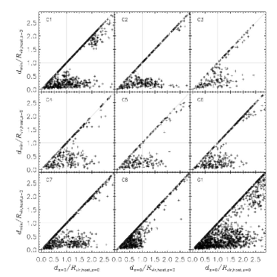
Figure 1: Minimum distance of a subhalo versus present distance. Subhaloes in the lower right corner of the plot are ’backsplash galaxies’: they have once been inside the host, but now are sitting outside the virial radius. Subhaloes in the upper right part have never been inside the host, but most of them are approaching the host halo ($d_{z=0}=d_{\rm min}$, solid grey line). (compare with Figure 2 of Gill et al. 2005))

As noted by both Gill et al. (2005) and Moore et al. (2004) a prominent population of backsplash galaxies is predicted to exist in galaxy clusters. We now demonstrate that a backsplash population is also predicted to exist in galaxies. In Figure 1 we show for each subhalo its minimum distance with respect to the centre of the host halo as a function of its distance with respect to the centre at the present day; both are normalised with respect to the host’s virial radius at redshift $z=0$.

Figure 1 reveals that backsplash subhaloes are also present in our galaxy mass halo. The backsplash population occupies the bottom right rectangle, with $d_{z=0}\geq 1R_{\rm vir,host,z=0}$ and $d_{\rm min}\leq 1R_{\rm vir,host,z=0}$. For the clusters, about 50% of the subhaloes within a distance $d\in[R_{\rm vir,host},2\,R_{\rm vir,host}]$ once passed through the virial sphere of their respective host. For the galactic halo G1, this figure rises to 63%. We note that the concept of the backsplash subhalo can partly be ascribed to the difficulty in choosing a good truncation radius for the host halo: the virial radius is more or less an arbitrary definition for the outer edge of a halo (cf. Diemand et al. 2006) and it has been shown by others that bound objects (in isolation) may as well extend way beyond this formal point-of-reference (Prada et al. 2006).

host	$n\ (R_{\rm vir})$	$n_{\rm bs}\ (2\,R_{\rm vir})$	$n_{\rm bs}/n_{\rm all}\ (2\,R_{\rm vir})$
C1	325	149	43%
C2	168	098	55%
C3	093	054	59%
C4	136	084	56%
C5	122	050	62%
C6	148	075	46%
C7	326	163	57%
C8	477	022	19%
G1	606	425	63%

Table 2: Number of subhaloes inside the virial region of the host ($n$), backsplash subhaloes between 1 and 2 virial radii ($n_{\rm bs}$) and the fraction of backsplash subhaloes in that region (with respect to all subhaloes between 1 and 2 virial radii). Only subhaloes containing at least 20 particles are counted.

The numbers of backsplash subhaloes for each host are given in Table 2, along with the number of trapped subhaloes. We note that the number of subhaloes is slightly larger than is given in Warnick & Knebe (2006), reflecting differences in how subhaloes are identified. In the previous study we used AHF, which identifies a “static” distribution of subhaloes in a single snapshot, whereas in the present study we use the halo tracker AHT (see Gill et al. 2004, for more details).

Interestingly, the fraction of backsplash subhaloes within one and two virial radii of the host varies between 43% and 63% for all hosts, except for the youngest system C8. There we find a rather low fraction of only 19%. This host is not only the youngest, but also an ongoing triple merger providing the most ’unrelaxed’ environment amongst our suite of hosts (cf. $Q$ value in Table 1). Thus maybe there are some potential backsplash subhaloes which simply did not yet have the time to leave their host again.

4.2 Mass Loss from Trapped Subhaloes

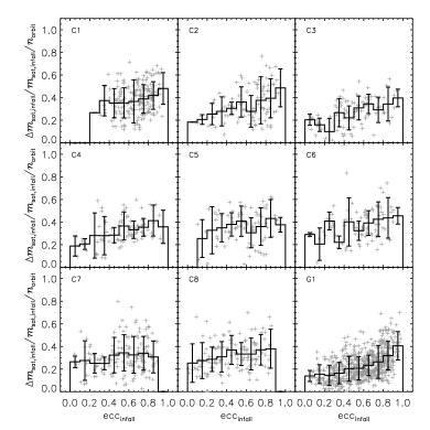
Figure 2: Fractional mass loss per orbit since infall time as a function of infall eccentricity. Subhaloes were selected according to the criteria: $\geq 1$ orbit, $n_{\rm part}\geq 20$ particles today and they must reside inside the host today.

Before investigating tidal debris fields it is necessary to quantify the actual mass loss. Are our subhalo systems actually losing mass and how does this mass loss relate to orbital parameters such as infall eccentricity? To answer this question we show in Figure 2 that trapped subhaloes on more eccentric orbits experience in general larger mass loss. We plot the total mass loss since infall time normalised to the initial mass divided by the number of orbits as a function of orbital eccentricity. The orbital eccentricity is derived here from the first apo- and pericentre distance of the subhalo’s orbit, after the subhalo entered the host region. This “infall eccentricity” might deviate strongly from the present value, since the eccentricity usually is evolving within time (see e.g. Hashimoto et al. 2003; Gill et al. 2004; Sales et al. 2007).

While in general all of the trapped subhaloes lose about 30% of their mass per orbit, some objects on radial orbits may lose up to 80% per orbit or even more. We like to note that only surviving haloes ($\geq 20$ particles) enter these plots and completely disrupted ones were not considered, respectively. Furthermore, only objects with at least one orbit were taken into account for Figure 2 as we needed one orbit to get a reliable measure for the (infall) eccentricity and the number of orbits.

4.3 Mass Loss from Backsplash Subhaloes

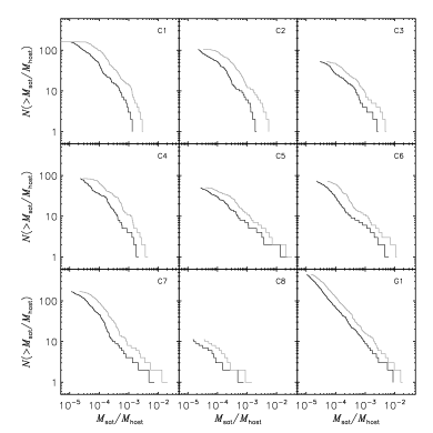
Figure 3: The cumulative mass function of the backsplash galaxies at redshift $z=0$ (heavy lines) and when using the mass at the infall time of each individual backsplash galaxy (faint lines).

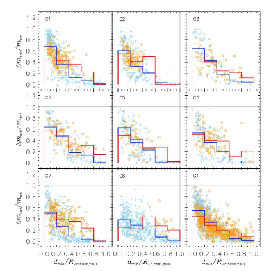
Figure 4: Fractional mass loss from subhaloes since infall time versus the normalised minimum distance to the host. Only surviving subhaloes are plotted. Trapped subhaloes are presented by blue plus signs, backsplash galaxies are marked by orange diamonds.

The results of the previous subsection show that trapped subhaloes suffer mass loss whose rate is enhanced for systems on more radial orbits. We now examine mass loss from backsplash subhaloes.

In Figure 3 we show the cumulative mass function of all backsplash subhaloes at redshift $z=0$ (heavy lines) and compare with the mass function of these subhaloes at their time of infall onto their host (faint lines). The two sets of mass functions approximately preserve their shape and differ effectively only in horizontal offset – the $z$=0 mass function can be obtained by a shift to the left of the mass function at infall. Further inspection of the figure reveals that every backsplash galaxy loses on average half its mass as it travels within the virial radius of the host and out again, irrespective of its original (infall) mass, i.e. the mass functions presented for each host halo in Figure 3 are self-similar.

Although backsplash subhaloes may not count as “true” subhaloes of the host, they experience mass loss within the host and therefore contribute to the tidal debris fields that we study in Section 5 and Section 6. We verify this in Figure 4, similar in spirit to Figure 2, where we plot the total mass loss from a subhalo over its full orbit since infall time as a function of minimum distance in terms of current host radius. We separate trapped and backsplash subhaloes by plotting the former with blue plus signs and the latter with orange diamonds. This figure demonstrates that subhaloes that have small pericentres with respect to the centre of the host experience greater mass loss, regardless of whether the subhalo is trapped or backsplash. We show also the average mass loss at a given minimum halocentric distance by the histograms in Figure 4. Interestingly, it is noticeable that backsplash subhaloes (orange) that grazed the outer regions of the host suffer greater mass loss than trapped subhaloes (blue) that reside in the same region.

host	$n_{\rm p}$	$n_{\rm p,sat}/n_{\rm p}$	$n_{\rm p,debris}/n_{\rm p}$	$n_{\rm p,sat}/n_{\rm p,debris}$	$n_{\rm p,bspl}/n_{\rm p}$	$n_{\rm p,bspl}/n_{\rm p,debris}$
C1	1810607	07%	20%	0.34	0.39%	02%
C2	884488	08%	08%	0.96	0.59%	010%
C3	672442	05%	21%	0.23	0.36%	02%
C4	870732	07%	010%	0.69	0.28%	05%
C5	744868	04%	22%	0.18	0.58%	05%
C6	879644	11%	25%	0.44	0.52%	03%
C7	1798507	12%	02%	4.89	0.16%	13%
C8	1906744	36%	20%	1.81	0.02%	00%
G1	2227123	07%	12%	0.60	0.67%	06%

Table 3: Number of particles inside the virial radius of the host (at $z=0$): $n_{\rm p}=$ total number, $n_{\rm p,sat}=$ the number of particles in still existing subhaloes ($\geq 20$ bound particles), $n_{\rm p,debris}=$ total number of particles in debris (including destroyed subhaloes and debris from backsplash galaxies), $n_{\rm p,bspl}=$ debris particles from backsplash subhaloes alone and the last column provides the ratio of the latter two numbers.

This figure also underlines our previous assertion that backsplash galaxies contribute to the overall tidal debris field. Table 3 quantifies this: at most 13% of the debris particles found within the host originate from backsplash subhaloes.

Table 3 gives the fraction of particles in subhaloes, debris and backsplash galaxies: our hosts’ masses in general consist of about 5 to 10% (in mass) from surviving subhaloes while 10 or 20% of the mass is contained in debris particles. A mere 0.5% of the total host mass originates from debris of backsplash galaxies. We further make the following observations about the subhalo and debris fractions of individual hosts.

• We note that the subhalo fraction in C8 is high, reflecting its involvement in a recent merger. Because a single massive subhalo persists (in fact, one of the most massive progenitor of the host) that has not yet merged, the subhalo mass fraction is close to 36%.

• The debris fraction for host C6 amounts up to nearly 25% because this host contains several massive subhaloes. We checked the initial subhalo mass function, i.e. the mass function of all trapped subhaloes at the formation time of the host, and indeed C6 contains initially more mass in subhaloes than any of the other hosts. The subhalo destruction rate is similar for all hosts and so the high debris fraction reflects the number of massive subhaloes that were present within the host at its formation time, rather than reflecting enhanced disruption of subhaloes within the host.

• In contrast, C7 is a host with a very low debris content, although it contains an average number of subhaloes. A detailed investigation of its temporal evolution revealed that neither the number of subhaloes nor the rate of subhalo disruption varies significantly with time. This is consistent with the small measured debris fraction.

It is instructive to compare our findings against the results of, for example, Diemand et al. (2006) and Gao et al. (2004). The former investigated mass loss per orbit as a function of pericentric distance (cf. their Fig.17) and arrived at the same conclusion: the closer a subhalo gets to the host’s centre, the greater its mass loss. A similar result was obtained by Gao et al. (2004) who found that subhaloes with large pericentric distance retains a greater fraction of their initial (i.e. infall) mass (cf. Fig. 15).

4.4 Summary – Subhaloes

Our study of the subhalo populations in the hosts reveals that backsplash subhaloes are present in both galaxy and galaxy cluster haloes. Approximately half of the haloes between $1$ and $2$ virial radii are actually backsplash subhaloes. Both trapped and backsplash subhaloes suffer mass loss as they orbit within the dense environs of the hosts – between 30 to 80% of their mass per orbit. The rate of mass loss is enhanced for those subhaloes that follow highly eccentric orbits and for those subhaloes whose orbits take them to small halocentric distances. This is in good agreement with the findings of previous studies (e.g., Gao et al. 2004; Diemand et al. 2006).

This lost mass will contribute to the tidal debris field within the hosts. The fraction of a host’s mass that comes from this lost mass ranges from a few percent (C7) to about 25% (C6). This diversity reflects differences in the subhalo populations that were present at the formation time of the host, and differences in the accretion histories of the hosts. We note that the contribution of mass lost from backsplash subhaloes to the total debris inside the host halo region today amounts to at most 13%. However, we conclude that when observing the debris of subhaloes and searching for possible corresponding subhalo galaxies, the region outside the virial radius of the host galaxy should also be considered.

5 Tidal Streams I:
Uncovering Subhalo Properties

When a subhalo moves on its path around the centre of its host, tidal forces (mainly from the host) tear it apart, usually generating the formation of a leading arm ahead of the subhalo and a trailing arm behind it. These arms are not always clearly distinguishable; sometimes they are broadened to such a degree that only a rather smooth sphere of unbound particles remains. How does the morphology of the debris field depend on the subhalo and the host? Can we learn anything about the host halo or the subhalo itself by studying only its debris field?

At this point it is instructive to consider the recent studies of Peñarrubia et al. (2006) and Sales et al. (2007). Peñarrubia et al. (2006) investigated the formation and evolution of tidal streams in analytic time-evolving dark matter host halo potentials and showed that observable properties of streams at the present-day can only be used to recover the present-day mass distribution of the host – they cannot tell us anything about the host at earlier times. However, if the full six dimensional phase space information of a tidal stream is available, it is also possible to determine the total mass loss suffered by the progenitor subhalo. Sales et al. (2007) showed that the survival of a subhalo in an external tidal field depends sensitively on its infall mass. One of our primary interests is the relation between the debris field and the total mass loss of the progenitor subhalo as well as its orbital eccentricity.

In the following analysis we focus on subhaloes that are the progenitors for tidal debris fields that contain at least 25 particles. We have taken care to ensure that low-mass subhaloes are not artificially disrupted (because of finite time-stepping, force resolution, particle number) by verifying that the fraction of a subhalo’s mass in the debris field does not correlate with the mass of the subhalo at infall. If numerics were playing a role, then we would expect lower mass systems to show preferentially higher mass fractions in the debris field. We further remade all plots showing analysis of the debris fields restricting the minimum number of particles in the progenitor satellite to $N_{\rm min}=600$. We could not find any substantial differences between results and hence adhere to the original plots. We note that the plots obtained by using the more restrictive limit on the satellite’s mass appear like having randomly sampled the original data; that is, they show the same trends. However, we note that in some instances extreme outliers are removed.

5.1 Orbital and Debris Plane

Definition

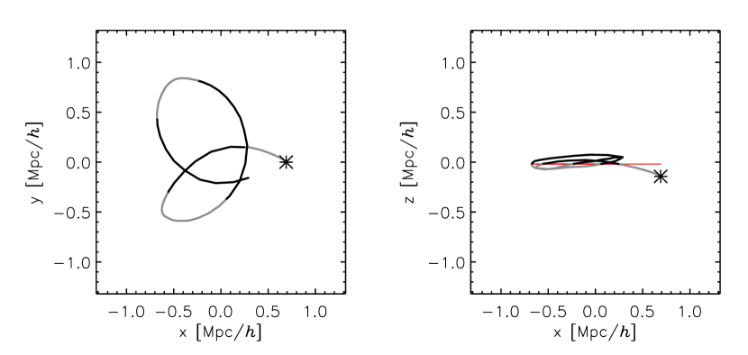
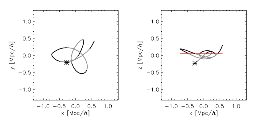
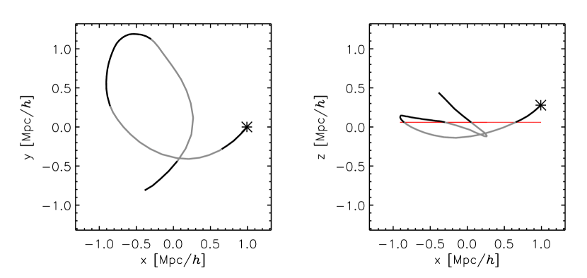
Figure 5: Fitting a plane to the orbit of three sample subhaloes in host halo C1. The left panel shows the orbit projected to its best fit plane, the right panel shows a perpendicular view, directly looking at the edge of the plane (straight red line). An asterisk marks the position of the subhalo today ($z=0$). The host halo’s centre is located at (0,0,0).

For an ideal spherical host potential the orbit of a subhalo (and therefore its debris field) is constrained to a plane (i.e. the orbital plane) because angular momentum is conserved. In non-spherical potentials, however, the orbit precesses out of the plane, and this leads to a thickening of the debris field in this direction (e.g. Ibata et al. 2001; Helmi 2004; Johnston et al. 2005; Peñarrubia et al. 2006). In addition to this effect, we expect the debris fields of more massive subhaloes and of subhaloes on highly eccentric orbits to show a greater spatial spread because they are more likely to lose more of their mass over a larger volume.

In order to quantify the deviation of both the subhaloes’ orbit and debris field from the orbital plane, we first determine a “mean orbital plane”, i.e. the best-fit plane to the orbit of the subhalo. Utilising all available orbital points for each individual subhalo (since infall time), we applied the Levenberg-Marquardt algorithm (see e.g. Press et al. 2002, Chapter 15.5) to minimise the distances of the points (without loss of generality) in $z$-direction. When using the general equation of a plane $E:ax+by+cz+d=0$ (with the normal vector $\textit{{n}}=(a,b,c)$), we obtain for a given $x$ and $y$ the expected $z$-value:

$$z = \alpha x+\beta y+\delta$$ (9)

$$\mathrm{with} \alpha=-\frac{a}{c}$$

$$\beta=-\frac{b}{c}$$

$$\delta=-\frac{d}{c}$$

$$c\neq 0$$

Employing the Levenberg-Marquardt algorithm then delivers the coefficients $\alpha$, $\beta$ and $\delta$ describing our best fit plane.

Examples of our fitting results are given in Figure 5. They illustrate how we can fit a plane to even a precessing orbit (cf. bottom panel). We have inspected visually many of our fits to orbital planes and we find that the “mean orbital planes” provide an adequate approximation .

Scatter about the orbit plane

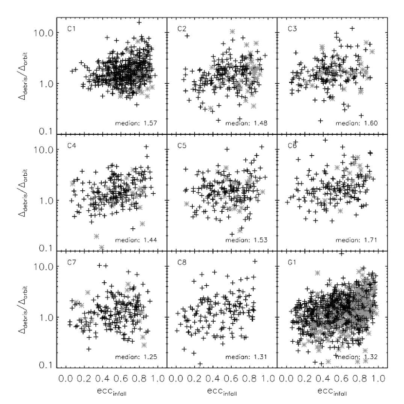
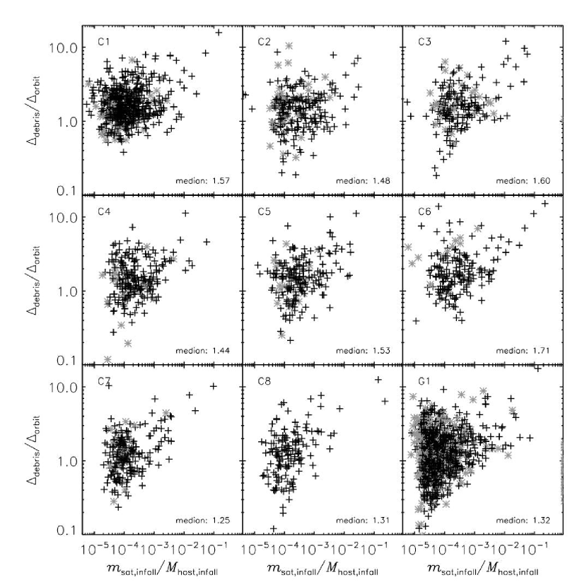
Figure 6: The deviation of debris particles from the best fitting orbital plane (with respect to the deviation of the orbit itself) as a function of infall eccentricity (left panel) and infall mass (right panel) for subhaloes with at least one orbit. Backsplash subhaloes are marked with grey asterisks. The median values of the distribution (trapped and backsplash galaxies together) are given in the lower right corner of each panel.

Given the best-fit orbital plane, we now have a means to quantify the deviation of the orbit itself from this ‘mean’ plane as well as the scatter of the debris particles about this plane. Using the orbital plane given by the equation $E:ax+by+cz+d=0$, we determine the perpendicular distance $\Delta_{i}$ of each orbit point/debris particle to the plane via the (general) equation

$$\delta_{i}=\left|\frac{a\,x_{i}+b\,y_{i}+c\,z_{i}+d}{a^{2}+b^{2}+c^{2}}\right|$$ (13)

The mean deviation of the orbit $\Delta_{\rm orbit}$ is determined using

$$\Delta^{2}_{\rm orbit}=\frac{1}{n-3}\sum_{i=0}^{n}\delta_{i}^{2}\quad.$$ (14)

The factor $(n-3)$ corresponds to the number of degrees of freedom, i.e. ‘number of data points ($n$)’ $-$ ‘number of free parameters (3)’.

For the scatter of the debris, we use an analogous formula for the mean deviation:

$$\Delta^{2}_{\rm debris}=\frac{1}{n_{\rm debris}-1}\sum_{i=0}^{n_{\rm debris}}\delta_{i}^{2}\quad.$$ (15)

Figure 6 shows the resulting debris scatter normalised to the deviation of the orbit itself for all chosen subhaloes in each simulation as a function of the infall eccentricity and the infall mass. Only subhaloes that have undergone at least one complete orbit inside the host halo are shown, since only then a reliable (infall) eccentricity determination based upon (first) apo- and pericentre of the orbit is possible. Disrupted subhaloes, or rather their debris, are also included in these plots. Subhaloes that once resided inside the host but are today found outside the host’s virial radius, i.e. the backsplash galaxies (see Section 4.1), are marked by grey asterisks. Interestingly, these are often the points deviating most from our expectation: we expect to observe a correlation of deviation with (infall) eccentricity, i.e. the larger the orbital eccentricity the greater the deviation of the tidal debris from the orbit.

Only a marginal trend is apparent that is most pronounced for the oldest systems (i.e. C1 and G1): C1, on the one hand, is one of those with a prolate shape, deviating more strongly from sphericity than most others. Thus, the large deviation of debris from the orbit plane could be a result of the flattened host halo as suggested by controlled experiments of disrupting subhaloes in flattened analytical host potentials (e.g. Ibata et al. 2003; Helmi 2004; Johnston et al. 2005; Peñarrubia et al. 2006). G1, on the other hand, contains the most subhaloes, thus encounters of debris streams with other sub-clumps are very likely, causing a heating of the stream which spreads the debris even more Moore et al. (1999); Ibata et al. (2002); Johnston et al. (2002); Peñarrubia et al. (2006).

The right panel of Figure 6 suggests that the trend is significantly more pronounced when plotting the deviation from the orbit plane against (infall) mass of the subhalo. Massive subhaloes always lead to large deviations of the debris about the orbital plane, whereas the debris of low mass subhaloes shows all kinds of deviations. We cannot construct a unique mapping of “debris deviation” onto “progenitor mass” by this method alone, but we note that it agrees with the findings of Peñarrubia et al. (2006), who claim that it is possible to infer the amount of mass loss from the stream’s progenitor using the full phase-space distribution of a tidal stream. We will return to this point later when studying the energies of stream particles.

Scatter about the debris plane

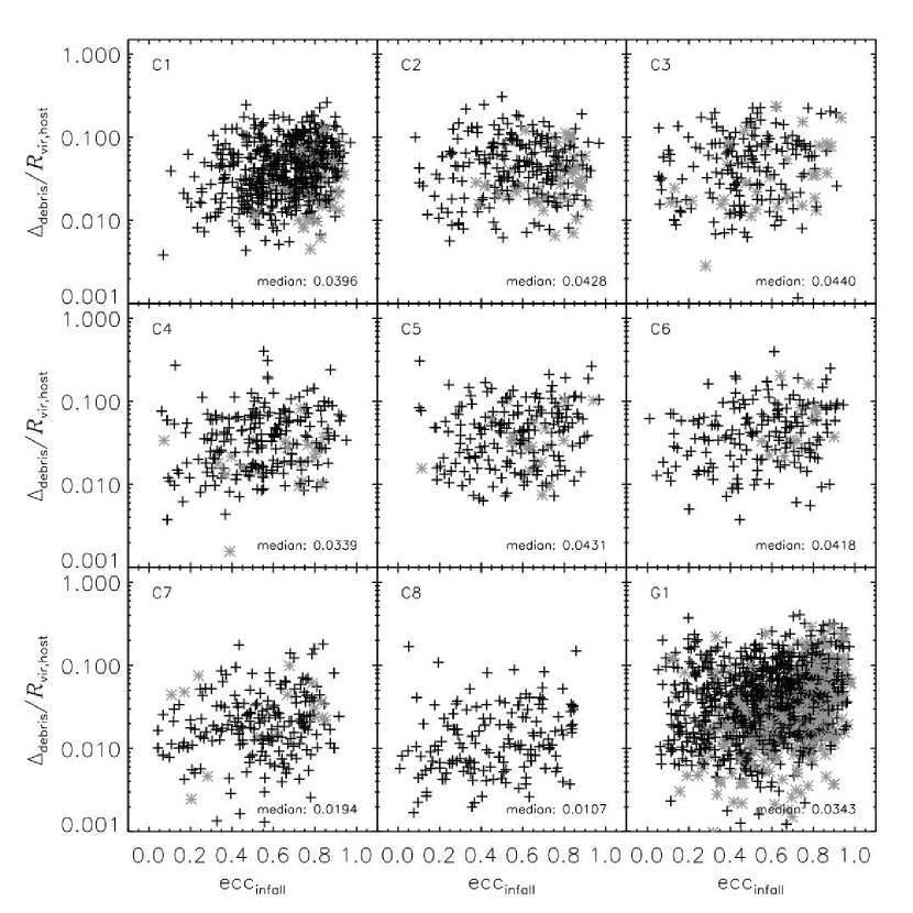
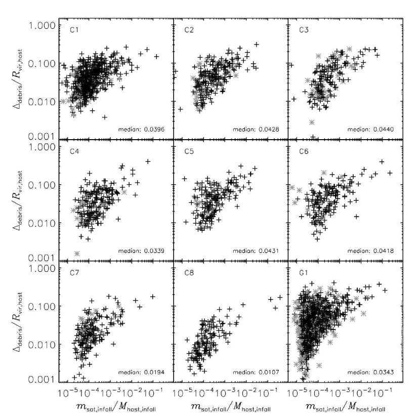
Figure 7: The deviation of debris particles from the best fitting debris plane (normalised to the virial radius of the respective host) as a function of infall eccentricity (left panel) and infall mass (right panel) for subhaloes with at least one orbit. Backsplash subhaloes are marked again with grey asterisks and the median values of the distributions are shown in the lower right corners.

An observer will not be able to recover the orbital path of a subhalo galaxy (without, for instance, semi-analytical modeling of its trajectory) and thus no information about the orbital plane will be directly available to him (or her). However, he (or she) could either define a plane based on the present subhalo’s position and velocity (i.e. the plane defined by the angular momentum vector) or fit a plane to the detected debris field and then determine the deviation of the debris field from this best-fit plane. We have adopted the latter approach and the result can be viewed in Figure 7 where we show the scatter of the debris particles about the best-fit debris plane versus infall eccentricity and mass. We note that the deviations of debris from a plane defined in this way are smaller than the deviations from the orbital plane. Again, only a marginal trend of increasing deviation for eccentric orbits is apparent. However, we now observe a stronger correlation between infall mass and debris deviation. Thus, by measuring the deviation of debris from the debris plane itself, it is possible for an observer to predict the most probable mass of the subhalo; in contrast, recovering the subhalo’s eccentricity will be more ambiguous.

The question arises as to why the correlation between (infall) mass and the debris variation is stronger in the case of the debris plane when compared to the orbital plane. Furthermore, we do not observe an “improvement” in the correlation with orbital (infall) eccentricity. We attribute this to the fact that the stream particles follow naturally the debris plane and hence show greater deviation from the orbital plane (that does not necessarily coincide with the debris plane); the debris plane is defined such that it minimises the scatter of the stream particles about that plane. Therefore, the correlation already apparent in Figure 6 strengthens when reducing the scatter in the deviation as is done when considering the debris plane rather than the orbital plane.

One may further argue that the destruction of subhaloes depends on their (infall) concentration and that more massive systems have lower concentrations (e.g., Bullock et al. 2001). We confirm the expected scaling between mass and concentration, although we find no correlation between (total) mass loss and (infall) concentration. Therefore, the trends seen in Figure 6 and 7 do not represent simple manifestations of the mass–concentration relation.

5.2 Tube Radius

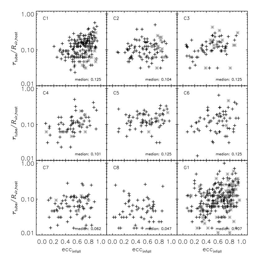
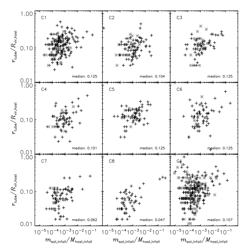
Figure 8: The tube radius as a function of infall eccentricity (left panel) and infall mass (right panel), normalised to the virial radius of the host today. Only subhaloes with at least one orbit and with a well-defined tube radius (# particles inside tube = $68.3\%\pm 2\%$) are plotted. Grey asterisks correspond to backsplash subhaloes again. Numbers in the lower right corner of each panel show the median values for both, trapped subhaloes and backsplash subhaloes together.

Even though the deviation from the orbital and debris plane may provide a means to infer the (infall) mass of a disrupting subhalo galaxy, we do not know whether the debris field is confined to the orbit or becomes completely detached from it. The work by Montuori et al. (2006) on tidal streams of globular clusters suggests that, in general, streams are good tracers of the orbit of their progenitor, at least on large scales. However, Choi et al. (2007) argue that the mass of the progenitor has a great influence: a massive subhalo gravitationally attracts the debris field, pulling it back and therefore causing a stronger bending of the arms. Thus, the streams should deviate strongly from the orbital path, the larger the mass of the progenitor subhalo is.

Furthermore, a large difference between the orbit and tidal streams may also indicate that the debris is just spreading over a larger area. This could then again be related to the infall eccentricity: subhaloes on spherical orbits will probably keep their streams quite close to the orbit, whereas subhaloes on radial orbits could have their debris spread to a much wider degree.

To quantify how debris relates to the orbit we introduce a “tube analysis” – we generate a tube about the orbital path of the subhalo, adjusting its radius $r_{\rm tube}$ such that $1\sigma$ (68.3%) of all debris particles are enclosed by the tube. Larger tube radii would then indicate that debris particles are deviating more strongly from the orbit of the subhalo. A detailed explanation of the “tube analysis” method and how to overcome its complications is presented in Appendix D.

The resulting tube radii (normalised to the host’s virial radius) as a function of eccentricity and mass are plotted in Figure 8. Subhaloes are ignored, if the tube radius did not converge satisfactorily (more than 2% deviation from the desired $1\sigma$ fraction of particles, mostly due to a small number of unbound particles). Again, only subhaloes with at least one full orbit are taken into account.

The expected trend of increasing tube radii with mass and eccentricity is a weak one at best and we conclude that such a tube analysis is less helpful in revealing subhalo properties than investigating the spread perpendicular to the debris plane. However, it nevertheless shows that the deviation of debris from the orbital path can be quite large. We therefore conclude that debris is not a well defined tracer of the orbital path of the progenitor subhalo as suggested by Choi et al. (2007).

We note also that in addition to studying how tube radii relate to subhalo properties, we examined how median tube radii related to the shape of the host. However, we were unable to identify any correlation.

5.3 Radial Velocity

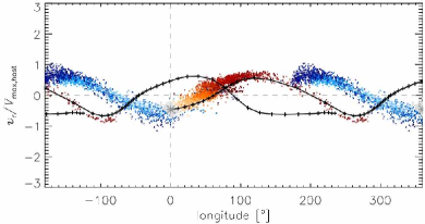
Figure 9: The radial velocity of subhalo #32 in host C1 (normalised to the maximum of the host’s rotation curve) versus longitude for an observer sitting in the centre of the host halo. Grey dots are bound particles, the black line shows the orbital path of the subhalo. Leading arm particles are coloured blue, trailing arm particles are shown in red with the brightness corresponding to the time since the particle became unbound (see Section 6 for more details). Note that we periodically wrapped the longitude extending the presented range from -180 to 360.

So far we have utilised the 3D position (and velocity) information available to us, but is interesting to ask how a subhalo stream would appear to an observer. An observer can, in principle, measure radial velocities of material in the tidal stream of a subhalo as well as its position on the sky. Let us imagine an observer positioned at the centre of a host halo, measuring the radial velocity of the (debris) particles of a certain subhalo in our simulations. We fix our coordinate system such that the plane best fitting the debris lies at zero latitude (i.e. zero height). A longitude of 0 shall correspond to the (remnant) subhalo’s position today. This enables us to plot an ‘observed’ radial velocity distribution versus longitude for a subhalo, as shown in Figure 9. Note that only debris particles lost after the infall of the subhalo into the host are considered; see Section 6 for more details. From this figure it is apparent that the arms are following a sine-like curve, just like the orbit (black line). The trailing arm (red) sits neatly on top of the orbit path in this example and the leading arm (blue) seems like a perfect continuation of the orbit to future times. This particular subhalo corresponds to one of the cases in the tube analysis that had a small tube radius. Its particulars are $N_{\rm orbit}=2.2$, ${\rm ecc}_{\rm infall}=0.458$, $M_{\rm infall}=8$, $M_{z=0}=1.6$, $M_{\rm trailing\ arm}=3.7$, $M_{\rm leading\ arm}=2.7$ (where masses are measured in $10^{11}$$h^{-1}{\ }{\rm M_{\odot}}$).

Such plots contain a remarkable wealth of information about the subhalo and its orbit. The maximum/minimum radial velocity are a direct measure of the eccentricity of the orbit: for circular orbits we would expect a constant line at $v_{\rm r}=0$; the more eccentric an orbit is, the larger are its minimum/maximum radial velocity (in absolute values). Furthermore they hint at the number of orbits a subhalo has already undertaken: each period which the sine-like curve of the debris describes corresponds to one half (debris) orbit. The phase-shift of successive sine-curves in these plots could also be used to infer the precession of tidal debris in the debris plane, which may be correlated with the triaxiality of the host halo. Also, the spread of each arm in radial velocity could also tell us something about the mass of the subhalo’s progenitor: more massive subhaloes will have a broader distribution of debris, in spatial terms as well as radial velocity (e.g. Choi et al. 2007).

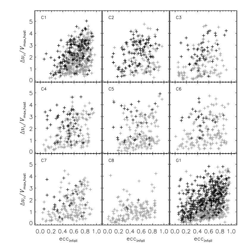
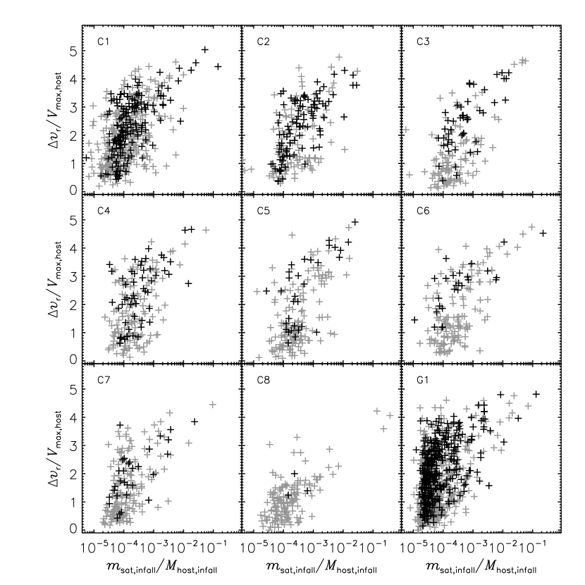
Figure 10: The spread in radial velocity of unbound particles (normalised to the maximum velocity of the rotation curve of the corresponding host) as a function of infall eccentricity (left panel) and normalised initial subhalo mass (right panel). The grey crosses correspond to subhaloes with $N_{\rm orbit}<3$ while the black crosses represent subhaloes with $N_{\rm orbit}\geq 3$.

However, for the moment we concentrate on the total spread of the radial velocity

$$\Delta v_{r}=v_{r}^{\rm max}-v_{r}^{\rm min}\ ,$$ (16)

and its relation to infall eccentricity and progenitor mass again. Figure 10 shows the difference between smallest and largest radial velocity measured for the corresponding subhalo’s debris as a function of infall eccentricity (left panel) and initial subhalo mass (right panel). Indeed we observe the expected trend, although the scatter is very large. We can also see that subhaloes with more than one orbit (darker plus signs in Figures 10) show a stronger signal: the more orbits undergone, the greater the probability that the difference in maximum and minimum radial velocity is determined by the orbital eccentricity rather than random scattering of the debris. But we also need to bear in mind that the debris field originating from subhaloes that have undergone a greater number of orbits will tend to be more massive, and therefore we would expect to make a more precise determination of $\Delta v_{r}$.

Using a more elaborate method for estimating the spread in radial velocity, such as using the mean values from the ten largest and smallest velocities or binning the distribution and taking the largest and smallest bin with a certain minimum number of particles, does not improve our results.

We now turn to the correlation between the spread in radial velocity and the progenitor’s infall mass (right panel of Figure 10); we do not expect to observe a strong correlation, because only the width of the streams themselves should depend on the mass, whereas the total spread correlates more strongly with orbital parameters. However, Figure 10 reveals quite a pronounced mass dependence: more massive haloes show a larger variety in radial velocities. Yet this correlation vanishes when looking at the radial velocity spread of the orbit itself (not shown here though). Thus, the signal found in Figure 10 suggests that the debris does not merely follow the orbit but spreads out to some angular extent that depends on its mass (compare also with the example radial velocity plot in Figure 9.). Again this shows that the stream itself is more sensitive to the mass of its progenitor subhalo than the orbital properties, as already suggested by the results of the previous subsections.

5.4 Summary – Uncovering Subhalo Properties

We set out to recover properties of the progenitor subhalo from its tidal debris field alone. Therefore we focused upon correlations between the tidal debris field and the progenitor subhalo’s infall eccentricity and mass.

Although the expected correlation with infall eccentricity is weak, the statistics that we have presented may nevertheless help to recover the orbit of an observed subhalo. Both methods (scatter about the debris plane and tube analysis) rely on measuring the debris field, thus allowing for a determination of the subhalo’s eccentricity. We therefore envision that a combination of both the debris scatter about the best fit debris plane and the tube analysis applied to existing stream data may help to refine models for the reconstruction of orbital parameters.

Relating the tidal streams with the original mass of the subhalo, we observed a noticeable correlation when using the deviation of the debris from the mean debris plane. This opens the opportunity to infer the original mass of a (currently) disrupting subhalo such as, for instance, the Sagittarius dwarf spheroidal Ibata et al. (1994). Using the relation between mass loss and eccentricity as presented in Figure 2, it may be possible to reconstruct the eccentricity of the orbit indirectly as soon as we know the original and present mass of the corresponding subhalo.

In addition, we presented an analysis of radial velocity plots as they might appear for an observer in the centre of a host. The spread in the radial velocity of the orbit itself is obviously strongly correlated with the (infall) eccentricity (not shown here), but it is less pronounced for the spread in debris (cf. Figure 10). It nevertheless shows a correlation with the mass of the progenitor, which is attributed to the fact that the debris of massive subhaloes actually spreads to a greater degree than for low-mass objects.

6 Tidal Streams II:
Separating Leading & Trailing Arms

So far the debris particles have been characterised by “bulk” properties, such as deviation from the orbital plane. No distinction has been made between leading and trailing arm or the time since the debris particles became unbound. In this section we investigate differences in the properties of both the leading and trailing arms, which makes it necessary to tackle the rather challenging task of assigning particles to the trailing or leading debris fields.

6.1 Age

We begin by defining the age of stream particles, in order to understand the build-up of the stream. We classify a particle as belonging to the stream at the moment at which it becomes unbound from its progenitor subhalo, which occurs when their velocity exceeds 1.5 times the escape velocity of the subhalo (see section 2.3). This age information is used to colour-code some of the following plots.

6.2 Membership to leading/trailing arm

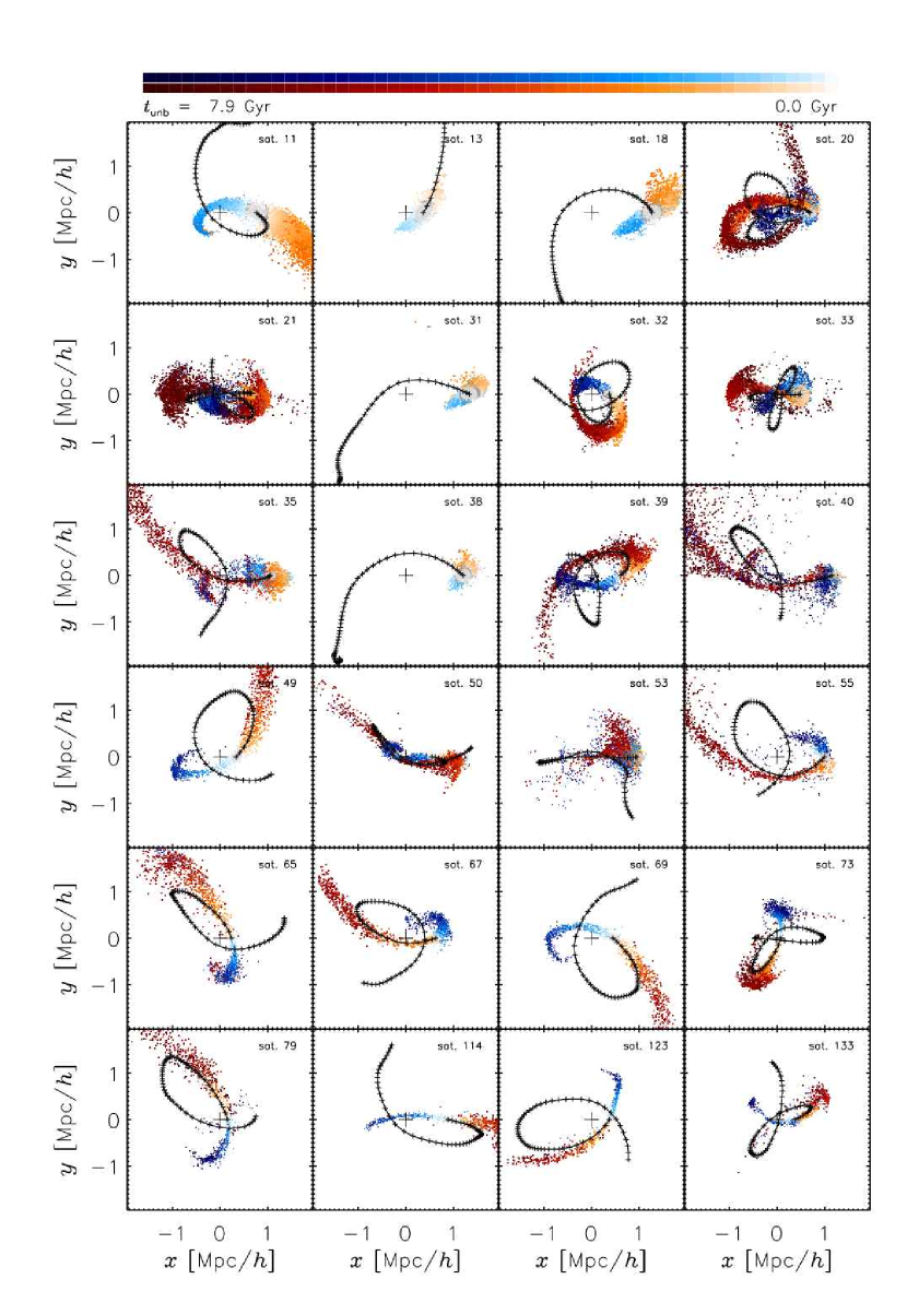
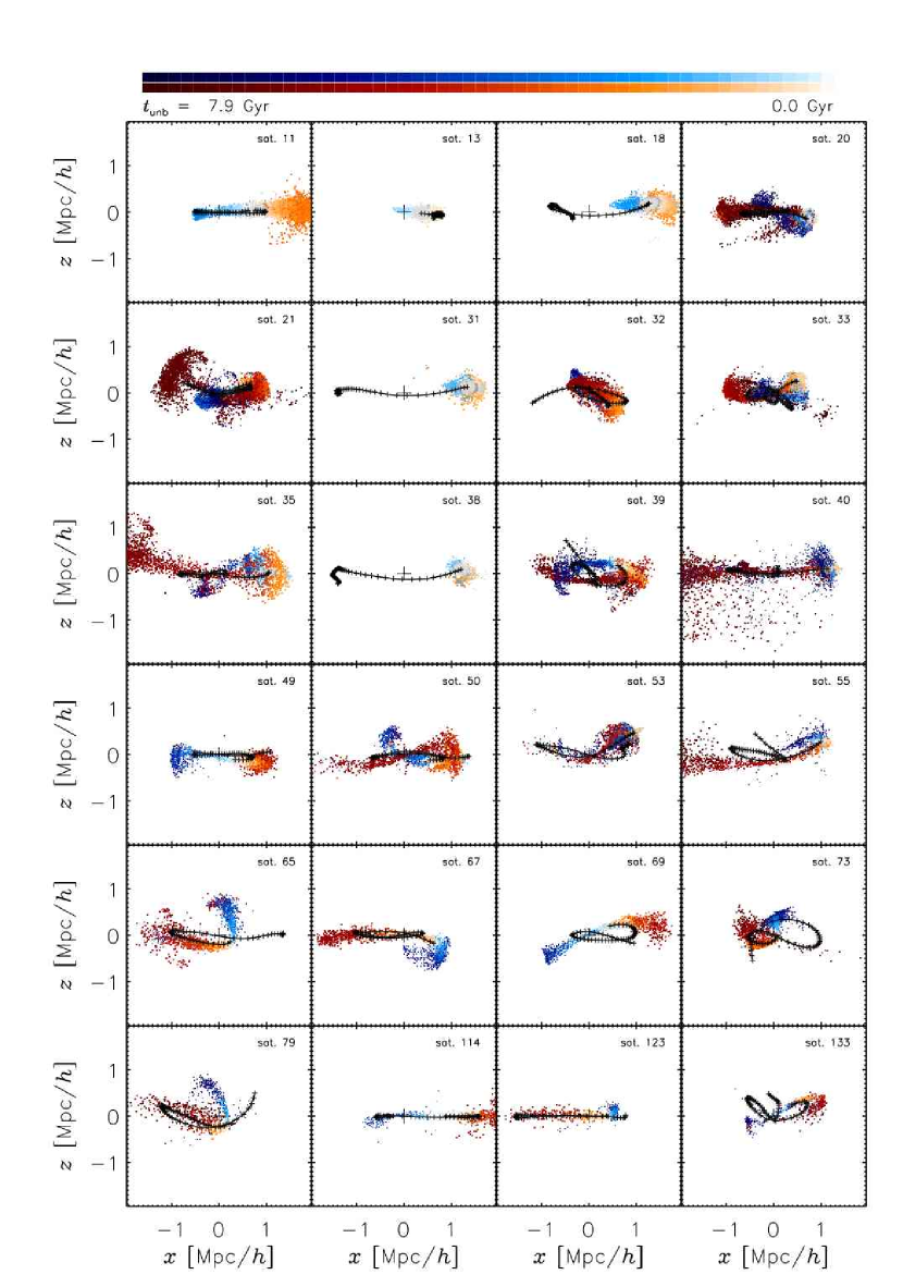
Figure 11: Classifying stream particles according to age and leading/trailing arm. Shown are the particles of a representative sample of subhalo galaxies orbiting in host C1 projected to their orbital planes (left panel) and as an edge-on view (right panel). The black line represents the path of the orbit. Grey particles are still bound to the subhalo, red particles are marking the trailing, blue ones the leading arm. The colours vary from dark to bright, indicating the age of the respective stream.

We require not only the age of stream particles but also a means to determine which of the arms, i.e. leading or trailing, the particle belongs to. For subhaloes with clearly distinguishable arms, one can separate leading and trailing stream easily by eye; however, an automated method that can objectively classify particles is both desirable and necessary, especially when analysing literally hundreds of subhaloes. We have developed such a method, which we now present.

For each snapshot, we mark particles leaving the subhalo in the “forward” direction as leading and those leaving in “backward” direction as trailing arm particles, where we define “forward” and “backward” as follows. If a particle leaves the subhalo, then – in a simplified picture – the subhalo has lost its influence on this particle; the host now plays the most important role and hence all subhaloes shall be neglected. In addition, the velocity of a recently unbound particle will still be close to the velocity of its progenitor subhalo. In the absence of any forces the particle would follow trajectory defined by the direction of the velocity vector, but it feels the gravitational pull of the host and therefore its direction is defined relative to the vector

$$\textit{{d}}=\frac{v^{2}}{r}\frac{\textit{{v}}}{v}-\frac{GM_{\rm host}(r)}{r^{2}}\frac{\textit{{r}}}{r}.$$ (17)

If a particle leaves the subhalo in this direction, it is tagged leading, otherwise trailing. For a subhalo moving at high velocity, a stream will form mostly along the orbit ($v^{2}$-term prevails), whereas the stream of a slow subhalo is more attracted by the host centre (see e.g. Montuori et al. 2006).

We note that using either the direction of the subhalo’s velocity (v) or the direction to the host (r) alone when distinguishing between leading and trailing arm particles does not give satisfactory results. Streams cannot be separated in this way because particles are not leaving simply in the direction of r or v.

Our leading/trailing classification method works well, as indicated by the example subhaloes presented in Figure 11 (see also the colors in the radial velocity plot, Figure 9, where the same classification procedure was used). It fails, however, for those subhaloes which have just recently fallen into the host. Here the subhaloes may have already lost mass before entering the host, due to interactions with adjacent subhaloes or other overdensities. Particles lost in such a way cannot be described by our (nevertheless simple) picture since the influence of other subhaloes is too large compared with the host halo’s influence. We therefore restrict the remaining analysis of debris to particles lost after their (progenitor) subhalo entered the host.

We note that Figure 11 provides further evidence that our procedure for fitting orbits to a plane as outlined in Section 5.1 works well for a variety of orbits.

6.3 Masses in streams

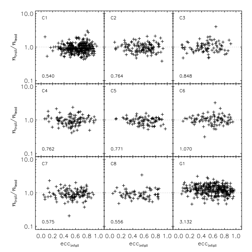
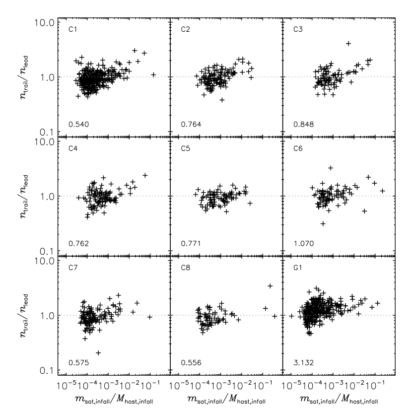
Figure 12: Ratio of the number of leading and trailing arm particles for subhaloes inside the host with at least one orbit, plotted versus the infall eccentricity (left panel) and infall mass (right panel). The number in the lower left corner of each panel gives the ratio of the number of subhaloes with a value above and below 1.

We are now in the position to explore differences in trailing and leading arm in detail and start with explicitly calculating the ratio of the mass in both arms. Figure 12 shows the ratio of the number of particles in the leading and trailing arm versus the infall eccentricity and mass of each subhalo. Again only subhaloes inside the host today and with at least one complete orbit (inside the host) are taken into account. Further, only subhaloes with at least 25 particles per arm are considered.

There appear to be slightly more particles in the leading than in the trailing arm in each of our cluster sized haloes while the reverse is true for the galactic halo G1. This is interesting because of the recent claim of Kesden & Kamionkowski (2006), who argue that if dark matter is coupled to dark energy, there must exist another force acting on dark matter particles besides gravitation. This additional force could manifest itself in non-equilibrium systems such as the tidal tails of subhaloes, leading to an imbalance in the mass of the leading and trailing arms. According to a simplified picture of tail formation in cosmologies without such coupling, both arms should contain the same amount of mass. Even though our simulations do not couple dark matter to dark energy, we observe a trend for an imbalance in the masses of leading and trailing arm. We therefore conclude that the proposition put forward by Kesden & Kamionkowski (2006) cannot hold in general.

In addition, we do not observe any tendency for the ratio of masses in leading and trailing arms to correlate with infall eccentricity, but we do note a trend for more massive subhaloes to lose more of their mass to the trailing arm. As Choi et al. (2007) have pointed out, the gravitational attraction of the subhalo on the tidal arms may cause an asymmetry in leading and trailing arm. The strength of this effect will increase with the mass of the subhalo, which can explain the mass dependence we observe. However, it is not clear why this ratio reverses for the galactic halo, although we note that the reversal is evident only for the least massive subhaloes.

6.4 Velocity dispersion in tidal streams

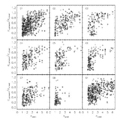
Figure 13: The velocity dispersion of trailing (black) and leading (dark grey) arm, normalised to the velocity dispersion of the host, as a function of the number of orbits. Since ’partial’ orbits at the beginning and end of the considered time interval are also taken into account, the number of orbits is not limited to integers.

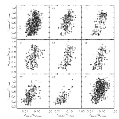
Figure 14: The velocity dispersion of trailing (black) and leading (dark grey) arm as a function of the deviation of debris from the best fit debris plane (compare with Figure 7).

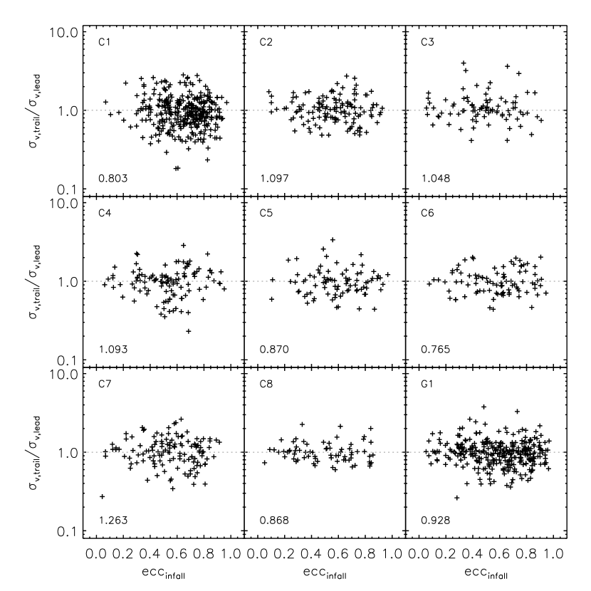
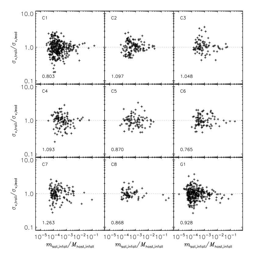
Figure 15: Ratio of the velocity dispersion in leading and trailing arm for subhaloes in the host with at least one orbit as a function of infall eccentricity (left panel) and infall mass (right panel).

The velocity dispersion of streams is another property that can reveal important insights to the history of the subhalo and characteristics of the host. For example, Johnston et al. (1996) note that a high velocity dispersion in the tail is suggestive of a massive progenitor as well as a high internal velocity dispersion in the original subhalo. However, the dispersion can increase further if the stream orbits in a “lumpy” host halo: encounters between the stream and sub-clumps will lead to dynamical heating of the stream. Furthermore, if the shape of the host deviates strongly from spherical symmetry, the subhalo and thus also its debris particles will start to precess, leading to yet further spread of the debris, increasing its spatial dispersion.

We start by exploring the relation between the number of orbits and the velocity dispersion in both the leading and trailing debris arm. The result can be viewed in Figure 13 where we find a general increase in the velocity dispersion with the number of orbits – the greater the number of orbits, the higher the velocity dispersion of the debris field. This figure is accompanied by Figure 14 where we show the relation between the velocity dispersion of debris and its scatter about the best fit debris plane (cf. Section 5.1). It underlines the trend that a larger deviation of the debris from the best fit plane correlates with a higher velocity dispersion and vice versa. Viewed in conjunction with Figure 6 (right panel) we recover the findings of Johnston et al. (1996) that a larger progenitor automatically leads to a higher velocity dispersion.

Are there differences in the velocity dispersions of the leading and trailing arms, induced by the host halo? In Figure 15 we show the ratio of the velocity dispersions in both tidal arms as a function of the subhalo’s infall eccentricity and mass again. We observe that the mean ratio is always of order unity with a roughly constant scatter when plotting against infall eccentricity, but the scatter decreases for initially more massive subhaloes (right panel of Figure 15). There appears to be only marginal differences between the leading and trailing arm with respects to the internal velocity dispersion. As they are spatially separated entities we therefore suspect interactions with sub-clumps in the host halo to have little influence unless both arms accidently encounter the same number of subhalo. It is more likely for the host to play the dominant role in the determination of the velocity dispersion of these two detached debris field.

6.5 Energy of tidal debris

We have learned that the masses of leading and trailing arm can differ, but their velocity dispersions are similar. While this may make it difficult to separate leading and trailing arms using raw velocity dispersions, we wish to understand whether we can use kinematic information to separate particles (or stars) into leading and trailing arms, as an observer might wish to do.

To this end, we present a method that allows classification into leading and trailing arms based upon the energy and angular momentum of tidal debris. Inspired by the work of Johnston (1998) who found a bi-modal energy distribution representative of leading (decrease in energy) and trailing arm (increase in energy) we calculate for each debris particle its change in total energy (also see McGlynn 1990; Johnston et al. 1999; Johnston et al. 2001; Peñarrubia et al. 2006). When combining the resulting distribution with our knowledge about the association of particles with leading/trailing arms we recover the findings of Johnston (1998) that there is a clear separation between the two arms in all our ’live’ host haloes – at least for the majority of subhaloes. In what follows, we focus on the properties of streams at $z$=0.

Energy of debris particles

The energy of a particle is simply the sum of its potential and kinetic energy. While it is straightforward to calculate the kinetic energy, the potential energy is always somewhat more complicated. We are left with the option to either use the AHF analysis of the simulation which leaves us with (more or less) spherically cut dark matter haloes or go back to the original simulation and derive the full potential used to integrate the equations of motion. As the former relies on assumptions that are not necessarily true for all our systems (i.e. we know quite well that our cosmological dark matter haloes are not spherical and better modeled by a triaxial density distribution) we chose to follow to the latter approach. This provides us with the most accurate measure for the potential energy we can get. We also mention that we estimate both the potential and kinetic energy in the rest frame of the underlying host halo. We understand that this approach works against any hypothetical observer, but we wish to maximise the possibility that there is any chance at all to separate particles into leading and trailing arm.

Energy scale

According to Johnston (1998) the changes in the total energy are of the order of the orbital energy of the subhalo itself. In order to scale the variation in the particles’ energies in a similar fashion we define this scale to be

$$\epsilon=\epsilon_{\rm pot}+\epsilon_{\rm kin}\ ,\$$ (18)

where $\epsilon_{\rm pot}$ and $\epsilon_{\rm kin}$ are the specific potential and kinetic energies of a test particle at the position and with the velocity of the (remnant) subhalo at redshift $z=0$. Note that for $\epsilon_{\rm pot}$ we interpolate the potential as returned by the simulation code AMIGA to the test particles’ position.

Energy distribution

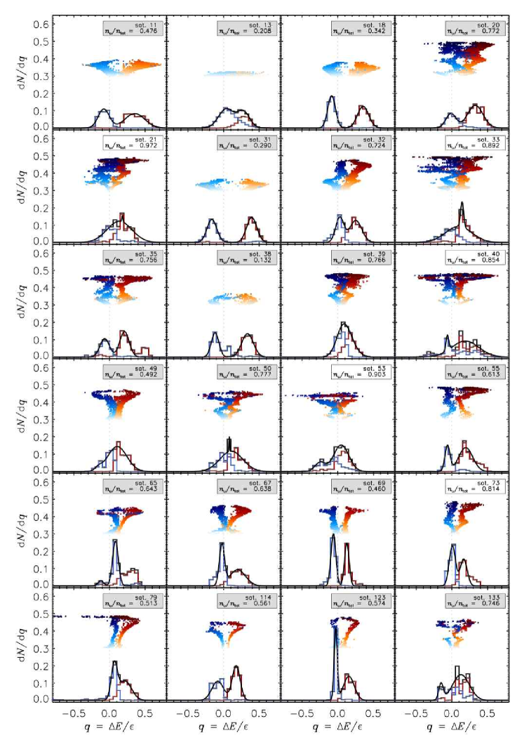
Figure 16: The distribution of energy change of debris particles for a random sample of subhaloes in the host C1. Please refer to the main text for details.

In order to be able to make predictions for an observer with access to the full 6D phase-space information for debris particles/stars and a realistic model for the host halo (in order to derive potential energies), we restrict the following analysis to quantities measured at $z=0$. We define the relative energy change of a debris particle to be

$$q=\frac{\Delta E}{\epsilon}=\frac{E-\epsilon}{\epsilon}\ ,\$$ (19)

where $E$ represents the particles total energy and $\epsilon$ the energy scale as defined above.

The resulting distribution for the same sample of subhaloes as already presented in Figure 11 can be viewed in Figure 16. This figure actually contains a substantial amount of information beside the energy distribution and hence requires careful explanation.

First of all, Figure 16, shows the distribution of $q$ as defined by Eq. (19). According to Johnston (1998) we should find a bi-modal distribution, at least for those subhaloes that are not yet completely disrupted. We therefore added the fraction of mass in the stream of the total mass to the legend (i.e. $n_{\rm u}/n_{\rm tot}$, where $n_{\rm u}$ is the number of unbound particles and $n_{\rm tot}$ the total number of particles left in the subhalo and $n_{\rm u}$ together). To further highlight non-disrupted subhaloes the legend box in the upper right corner is shaded in grey for objects where less than 80% of all particles are forming the debris field ($n_{\rm u}/n_{\rm tot}<0.8$). As we are in the unique position to separate leading and trailing arm debris using the method described in Section 6.2 we not only present the combined energy distribution (black histograms) but also the individual distributions for trailing (red histograms) and leading arm (blue histograms). The colour-coded dots above the histograms are the relative energies $q$ of each individual debris particle where the saturation of the colour corresponds to stream age as defined in Section 6.2, too.

While many of the energy distributions are clearly bi-modal (even for disrupted subhaloes), we notice that the dip in between the peaks is not necessarily located at $q=0$, which just means that our choice of the energy scale is not good enough. Nevertheless, we claim that (i) this distribution can be obtained observationally once the full 6D phase-space information (for at least a substantial amount of debris particles/stars) along with a sufficient model for the underlying host potential is available and (ii) subsequently be used to separate leading from trailing arm even if the debris is wrapped around the host and the progenitor subhalo had a number of orbits, respectively. One may claim that our model for the host potential is out of reach for an observer as we are using the exact potential values as returned by the simulation code, but we also applied the less sophisticated approach of using a simple spherically symmetric potential and were unable to detect significant differences in the respective energy distributions.

Another noticeable feature in Figure 16 are the “swings” in the particle distribution: these most probably correspond to the orbital motion of the subhalo. If we were scaling the particle’s energies with the corresponding energy scale when the particle became unbound or with the corresponding pericentre energy (as suggested by Johnston (1998)), these “swings” might vanish and we could possibly achieve a “cleaner” distribution. However, this energy scale would not be directly accessible to an observer.

Separating leading and trailing arm via energy

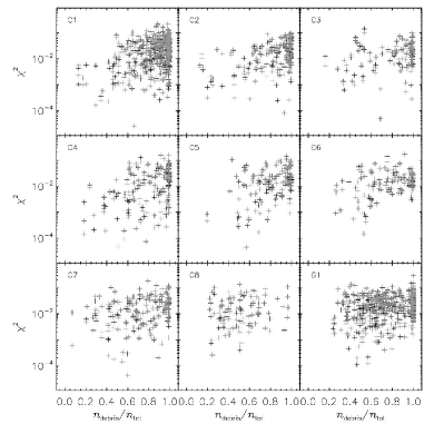
Figure 17: Reproducibility of leading and trailing arm energy distribution by decomposing a double-Gauss-fit: The goodness $\chi^{2}$ for trailing (black) and leading (grey) arm is plotted versus the fraction of debris particles.

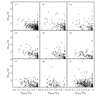
Figure 18: Separation of maxima and the fraction of debris particles. Grey: 80% or more particles in debris, black: 20% or more particles are still bound.

In order to check the credibility of our proposed method to classify a particle/star by its (relative) energy and assign it to either the leading or trailing arm we need to check the statistical significance of this technique. To this end we fitted a ’double Gaussian’ to the energy distribution of the subhaloes in all our nine host haloes

$$\frac{dN}{dq}=A_{1}e^{{-\frac{1}{2}\left(\frac{x-x_{1}}{\sigma_{1}}\right)^{2}}}+A_{2}e^{{-\frac{1}{2}\left(\frac{x-x_{2}}{\sigma_{2}}\right)^{2}}}\ ,\$$ (20)

where $A_{1},A_{2},x_{1},x_{2},\sigma_{1},$ and $\sigma_{2}$ are free parameters. The resulting best fit curves to the combined distribution $dN/dq$ for a number of sample subhaloes are given by the solid black lines in Figure 16.

To gauge the integrity of our claim that it is possible to separate leading and trailing arm using the energy distribution, we make use of the fact that we are in the unique situation to separate leading and trailing arm particles again. We therefore calculate for each arm the energy distribution individually. We further decompose the fit to the combined energy distribution based upon all particles in the debris field (cf. Eq. (20)) into two single Gaussian (i.e. one should describe the leading and the other the trailing arm). We check the validity of the decomposed Gaussians by comparing them to the corresponding “true” energy distributions derived via our “exact” leading/trailing arm classification method. Hence, for each subhalo we calculate two $\chi^{2}$ values representative of the squared deviations between the decomposed fit and the true (binned) distributions for leading and trailing arm. The results can be viewed in Figures 17, 18, and 19 to be explained in more detail below.

Johnston (1998) stated that the bimodality is in general more pronounced for subhaloes that are not disrupted, and for disrupted subhaloes a single-peaked distribution is expected. We therefore start by inspecting the quality of our double-Gaussian fits by plotting the respective $\chi^{2}$ values against the fraction of mass in the debris field, i.e. number of particles $n_{\rm debris}$ in the debris field over number of particles $n_{\rm tot}=n_{\rm debris}+n_{\rm sat}$ where $n_{\rm sat}$ are the remnant particles in the subhalo; a ratio of $n_{\rm debris}/n_{\rm tot}=1$ refers to a completely disrupted subhalo. The result is presented in Figure 17 where we observe a (marginal) trend for more disrupted subhaloes (i.e. larger $n_{\rm debris}/n_{\rm tot}$ ratios) to have higher $\chi^{2}$ values in agreement with our expectation and Johnston (1998), respectively. However, we find no difference for leading (grey symbols) and trailing (black symbols) arm.

In Figure 18 we plot the separation of the maxima of the two Gaussians (derived via fits to the distributions stemming from the separation method and not the decomposition of Eq. (20) versus the debris fraction $n_{\rm debris}/n_{\rm tot}$ again. The peak separation is further normalised to the sum of the half width at half maximum of each curve. We can confirm a small trend towards smaller separations for more disrupted subhaloes, i.e. the maxima are approaching each other and leading to less distinguishable curves for more disrupted subhaloes, as expected.

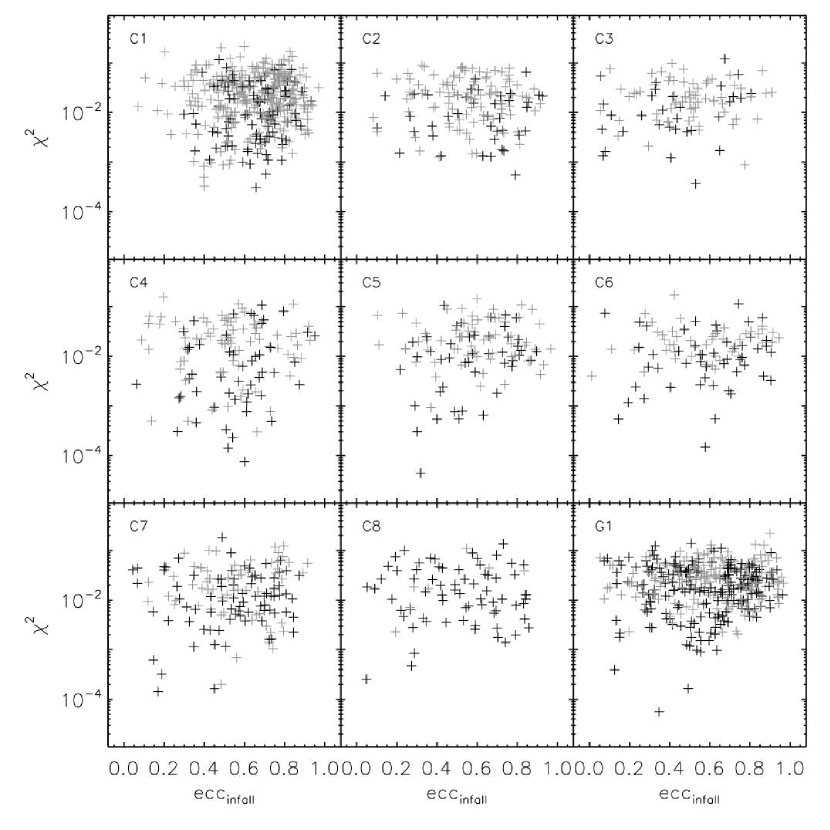
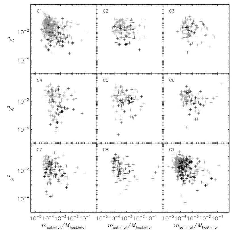
Figure 19: Correlation of the infall eccentricity (left panel) and infall mass (right panel) with the quality of the decomposition of the fit of the energy distribution into leading and trailing arm distribution. Grey (black) symbols mark disrupted (alive) subhaloes where the criterion for disruption corresponds to $n_{\rm debris}/n_{\rm tot}>0.8$ again.

Finally we turn to our two subhalo properties again, namely the infall eccentricity and infall mass, examining if or how they relate to the (bi-modal) energy distribution. We plot in Figure 19 the correlation of the infall eccentricity (left panel) and infall mass (right panel) with the quality of the decomposition of the fit of the energy distribution to a double Gaussian $\chi^{2}$. We (again) observe little relation with eccentricity while there is a trend for more massive subhaloes to lead to better fits and hence a clearer separation between leading and trailing arm. Please note that we separated the subhaloes in Figure 19 according to disrupted (grey symbols) and alive (black symbols), where our criterion for disruption was fixed at $n_{\rm debris}/n_{\rm tot}\geq 0.8$.

6.6 Summary – Leading vs. Trailing Arms

In this section we investigated trailing and leading arms individually working out differences and similarities between the debris fields. Somewhat surprisingly, most of the properties we considered show little (if any) variation between the arms (e.g. velocity dispersion), but there does appear to be a mass difference between them. Our main conclusion is that even for complicated geometries of both arms it is in principle possible to separate individual particles/stars amongst leading or trailing arms by means of their energy distributions. This in turn allows to (observationally) weigh both arms and verify our claim that their masses are different.

In short, our results of the analysis of leading and trailing arm properties can be summarised as follows:

• We presented a method to separate leading and trailing arm particles in cosmological simulations.

• We confirmed that the method to separate leading and trailing arm utilising the energy distribution works well in cosmological simulations.

• Trailing and leading arm can be separated observationally, when investigating the energy of debris particles: the energy distributions can be fitted by Gaussians, where the peak for the leading arm lies at smaller energies than the peak for the trailing arm.

• The leading arm contains slightly more mass than the trailing arm for more than half of the subhaloes in our cluster haloes, whereas the opposite relation holds for the galactic halo. For more massive subhaloes, the fraction of mass in the trailing arm is increasingly higher.

• We could not find differences in the velocity dispersions of leading and trailing arm.

7 Summary and Conclusions

In this paper, which is the first in a series, we have investigated the tidal disruption of subhaloes (or satellite galaxies) orbiting in cosmological dark matter host haloes. We used nine high resolution cosmological $N$-body simulations of individual galaxy- and cluster-mass haloes, each of which contain in excess of $\sim 1$ million particles within the virial radius, and within which a few hundred subhaloes can be reliably resolved. The time sampling of our simulations is such that we can track subhalo orbits in detail, which allows us to both determine orbital planes for subhaloes and to follow the mass loss they suffer as a function of time.

In the first part of the paper (i.e. Section 3) we concluded that, while all of our host haloes are sufficiently relaxed, they exhibit a range of integral properties. For example, they show a spread in formation times, mass assembly histories and shapes. These are precisely the kind of host properties that we expect to affect the properties of tidal debris field stripped from orbiting satellites.

The second part of the paper (i.e. Sections 4–6) focused on the subhaloes and their tidal disruption. Our main conclusions may be summarised as follows;

• We predict that “backsplash” satellite galaxies should be found not only in the outskirts of galaxy clusters but also around galaxies.

• Backsplash subhaloes contribute as much as 13% of the mass of the total tidal debris field within the host. This suggests that the region outside the virial radius of the host galaxy should be considered also when observing the debris of satellites and searching for possible corresponding satellite galaxies.

• Tidal stream properties correlate well with progenitor satellite properties. For example, we find a relationship between the scatter about the (best-fit) debris plane and the infall mass of the satellite, as well as the spread in radial velocity and the infall eccentricity.

• We devised a method to separate leading and trailing debris arm in cosmological simulations.

• The masses of leading and trailing arms differ.

• We do not find differences in the velocity dispersions of leading and trailing arms.

• We present a method that uses energy distributions to separate leading and trailing arms and that can, in principle, be employed by observers.

• The formation of the tidal debris field is extremely complex in “live” host haloes such that there appears to be little correlation between debris properties and host halo properties (age, mass assembly history, dynamical state, shape).

We set out to address two central questions key to understanding tidal streams;

• Can observations of tidal streams be used to infer the properties of their parent satellite?

• Can tidal streams reveal properties of the underlying dark matter distribution of the host halo?

These have proven to be very weighty questions to address, and so we focused on the first question in this paper. As the bullet points above indicate, the answer would appear to be yes. For example, there is a clear correlation between mass loss and orbital infall eccentricity, and between deviation of the tidal debris field from its orbital plane and the infall mass of the progenitor satellite. Addressing the second question is less straightforward. We have examined our data for correlations between stream properties and host properties as summarised Table 1, but evidence for correlations with host mass accretion history, dynamical state and shape are extremely weak at best. Indeed, the only suggestion of a correlation that we find is between the mass ratio of leading to trailing arm and the virial mass of the host; while all our cluster mass haloes have more mass in the leading debris arm, the relation is reversed in the galaxy mass halo.

Further, it is interesting to note that the galaxy halo G1 appears to be distinct from the eight galaxy cluster haloes (with the possible exception of C1) in terms of how its bulk properties relate to its stream properties. However, it is not clear whether this is a systematic effect, given that G1 is the only realisation of a galactic type halo. For example, the differences are not so striking if one compares G1 with C1. We are in the process of building a sample of galaxy haloes to supplement G1.

We now conclude with some general remarks. Previous studies of individual satellites disrupting in analytic host potentials using controlled $N$-body experiments have hinted at simple and direct links between, for example, the flattening of the host potential and the dispersion of the debris field (e.g., Ibata et al. 2003; Helmi 2004; Peñarrubia et al. 2006). However, our experience suggests that the situation is vastly more complicated in “live” host haloes, where the host undergoes a complex mass accretion history, contains a wealth of substructure and cannot be easily modeled as a simple ellipsoid. Peñarrubia et al. (2006) pointed out that all present-day observable stream properties can only constrain the present mass distribution of the host halo, independent of its past evolution. We would argue strongly that even present-day properties of the host halo will be difficult to infer from stream properties, given the complexity of interactions responsible for the emergence of debris fields. There are multiple processes driving these effects and so while we note tentative correlations, we require further simulations to help us understand what is happening. This will represent the focus of the following paper in this series. We point out that this situation is akin to the findings of Gill et al. (2004); they presented a detailed study of the dynamics of satellite galaxies in similar host haloes and were also unable to establish correlations to the host properties.

We close with a cautionary note: this paper is not to be understood as a definitive quantitative analysis of tidal streams in dark matter haloes. Rather it shows that certain (unexpected) correlations between the debris field and satellite properties exist. Our study therefore represents the first step towards our understanding of whether or not tidal streams from disrupting satellite galaxies can be used to deduce robustly properties of their host dark matter haloes and of the orbits of the satellites.

Appendix A Measuring Halo Shapes: A New Approach

A.1 Motivation for our Approach

There is a rich literature on methods for the determination of halo shapes. Many of these studies utilise methods that identify subsets of particles and deduce axis ratios and orientations of best fitting ellipsoids to the haloes from the eigenvalues and eigenvectors of the moment of inertia tensor of the particles (e.g., Frenk et al. 1988; Jing & Suto 2002) . However, the predicted shape depends on what is measured. Typically particles are selected according to radius (e.g. Frenk et al. 1988) but they can also be selected according to local density (e.g. Jing & Suto 2002) or potential (e.g. Power 2003), with differing results. The presence of substructure within haloes also affects the measured shape (e.g. Bailin & Steinmetz 2005). We wish to develop a method that produces an unbiased estimate of a dark matter halo’s shape and orientation and that is unaffected by substructure.

A.2 Isodensity and Equipotential Surfaces

It can be argued that the shape of the potential rather than the mass density provides a more meaningful measure of the shape of the halo for our purposes, because it is the potential that determines the orbits of satellites and tidal debris (e.g. Hayashi et al. 2007). We use a novel technique to define both isodensity and equipotential surfaces while simultaneously allowing identifying a corresponding (spherical) radius $R_{\rm iso}$ with the given surface.

Our method for locating particles on isodensity/equipotential surfaces is as follows;

• We start by calculating the local value of the density and potential at each particle position. To this extent we invoke again the original adaptive grid hierarchy used during the actual simulation, obtain the density and potential on these grids and interpolate to the particle positions.

• We select a fiducial radius $R_{\rm iso}$. We then successively increase the thickness $\Delta R$ of a spherical shell centred about the fiducial radius $R_{\rm iso}$, i.e. the shell extends from $R_{\rm iso}^{\rm min}=R_{\rm iso}-\Delta R$ to $R_{\rm iso}^{\rm min}=R_{\rm iso}+\Delta R$. The value of $\Delta R$ is determined in a way that we require to include a certain fraction of the total number of halo particles in the shell; in our case this amounts to 10%.

• For all the particles in the shell we calculate the mean value of the density (potential). This now defines the threshold isodensity (equipotential) value at our fiducial radius $R_{\rm iso}$.

• From all simulation particles in the vicinity of the host (i.e. out to 2.5 $R_{\rm vir}$) we now pick those ones whose local density (potential) value lies within a range of 10% about the mean value.

A.3 Shape Determination

Having identified the subset of particles with the desired local density (potential) at $R_{\rm iso}$ (cf. Section A.2), we compute their moment of inertia tensor $I_{jk}$. The eigenvalues and eigenvectors of $I_{jk}$ are related to the axis ratios and orientation, respectively, of the best-fitting ellipsoid to the particles. For a distribution of discrete point masses, $I_{jk}$ is expressed as

$$I_{jk}=\sum_{i=1}^{N}m_{i}(r^{2}_{i}\delta_{jk}-x_{ij}x_{ik})\quad\\ {\rm with}\ j,k=\{1;2;3\}\quad,$$ (21)

where $m_{i}$ is the mass of particle $i$, $N$ the number of particles and $r_{i}=\sqrt{x_{i1}^{2}+x_{i2}^{2}+x_{i3}^{2}}$ is the distance of particle $i$ from the centre of mass of the particles.

The novelty in our method of determining the shape is that we weigh particles by their local density when computing $I_{jk}$ as follows;

$$I_{jk}=A\cdot\sum_{i=1}^{N}\frac{1}{\rho_{i}}(r^{2}_{i}\delta_{jk}-x_{ij}x_{ik})\quad\ \ {\rm with}\ j,k=\{1;2;3\}.$$ (23)

Here $\rho_{i}$ is the local density of particle $i$ and the normalisation factor $A$ is given by,

$$A=\frac{1}{\sum_{i}{1/\rho_{i}}}\cdot N\ .\\$$ (24)

This is necessary to ensure that especially particles in equipotential shells, which can have a substantial spread in their local densities, have approximately equal weighting in the summation. If this weighting is neglected, particles in higher density regions will dominate the summation and will bias our estimate of the axis ratios of the best-fitting ellipsoid. The formula for obtaining the correct axis lengths $a>b>c$ from the eigenvalues of this inertia tensor is given in Appendix B below.

As our host haloes contain a considerable amount of substructure which may distort the determination of the host’s shape, we performed the shape analysis with as well as without removing all subhalos (i.e. all bound spherical halos found by the AHF analysis) from the host. We found that these subsystems do in fact have a great influence on the shape (especially on the shape of the potential) and thus we removed them for a credible and unbiased shape determination.

Our shape determination of all nine host haloes is presented in Appendix C where we show the best fit ellipsoid to both the equipotential (upper panels) and isodensity (lower panels) contours at $R_{\rm iso}=R_{\rm vir}$.

We further calculate the usual measure for triaxiality $T=(a^{2}-b^{2})/(a^{2}-c^{2})$ and list the values for both $T$ and $c/a$ (sphericity measure) at $R_{\rm iso}=R_{\rm vir}$ in Table 1.

A.3.1 Comparison to Previous Methods

The simplest method determines the shape and orientation of a halo using all particles within a spherical volume or shell at a given radius (e.g. Frenk et al. 1988; Kasun & Evrard 2005; Hopkins et al. 2005; Bailin & Steinmetz 2005). While this method robustly recovers the orientation of the halo, the resulting axis ratios tend to be biased towards larger values (i.e. haloes are predicted to be rounder).

An alternative iterative approach to the problem again determines the shape and orientation of a halo using all particles within a spherical volume or shell, but this initial surface or shell is now deformed in the direction along the principal axes of the best fitting ellipsoid; this process is repeated until convergence is achieved (e.g. Katz 1991; Dubinski & Carlberg 1991; Warren et al. 1992; Bullock 2002; Allgood et al. 2006; Macciò et al. 2006). Both Jing & Suto (2002) and Bailin & Steinmetz (2005) have noted that iterative methods have difficulty in achieving convergence in simulations in which haloes are very well resolved and contain a population of satellites. Satellites tend to lead to a distortion of the shape, and this is most pronounced in the outermost parts of host haloes where recently accreted satellites are most likely to be found.

The impact of substructure can be reduced by working with a “reduced inertia tensor”;

$$\hat{{\cal M}}_{jk}=\sum_{i=1}^{N}\frac{m_{i}x_{ij}x_{ik}}{r_{i}^{2}}\ .$$ (25)

Here each particle is weighted by the inverse square of its distance to the centre of the halo. While this recovers accurately the orientation of the ellipsoid, the axis ratios are systematically overestimated and thus haloes are predicted to be more spherical than they actually are (e.g. Bailin & Steinmetz 2004).

Both of these approaches have in general been applied in studies in which the best resolved haloes contain several tends of thousands of particles at most, in which it is not possible to defined thin shells containing many particles with similar local densities or potentials. A couple of studies (Jing & Suto 2002; Power 2003) have looked at the shapes of well resolved haloes, each containing several hundred thousand particles within the virial radius. They identified shells of particles selected by local density and potential and determined the best fitting ellipsoids. While this approach is similar to the one we have adopted, we note that these authors selected particles according to a local density or potential threshold.

A.3.2 Advantages of Our New Approach

The method presented in Appendix refapp:isoequi enables us to select particles explicitly according to both their radius with respect to the centre of the halo and their local density (potential). This is desirable for a number of reasons.

• It overcomes the problems of convergence faced by iterative methods and it avoids the artificial bias towards more spherical shapes introduced by the reduced inertia tensor (equation 25).

• By focusing on thin shells, we can obtain uncorrelated results for the shapes in the inner and outer parts of haloes.

• By fixing the radius at which we select particles rather than fixing the local density or potential threshold of particles (as in Jing & Suto 2002; Power 2003), we can compare directly the shape of the local density and potential at the same radius.

• We can compare the shapes of different haloes at the same fraction of the virial radius, which depends solely on virial mass, rather than at a similar local density or potential, which will depend on concentration, recent merging history, larger scale environment, etc….

Appendix B Measuring Halo Shapes: From Eigenvalues to Ellipsoid Axes

When we diagonalise the moment of inertia tensor (as defined by equation 21) for a thin shell of particles, we obtain the “principal moments”,

$$\lambda_{1} = I_{x^{\prime}x^{\prime}}=M\sum_{i=1}^{N}(y^{\prime 2}_{i}+z^{\prime 2}_{i})$$ (26)

$$\lambda_{2} = I_{y^{\prime}y^{\prime}}=M\sum_{i=1}^{N}(z^{\prime 2}_{i}+x^{\prime 2}_{i})$$ (27)

$$\lambda_{3} = I_{z^{\prime}z^{\prime}}=M\sum_{i=1}^{N}(x^{\prime 2}_{i}+y^{\prime 2}_{i}).$$ (28)

Here $x^{\prime}$, $y^{\prime}$, $z^{\prime}$ are the coordinates in the principal axes frame, $M$ is the total mass of the shell.

For a thin ellipsoidal shell with major, intermediate and minor axes $a>b>c$, the corresponding principal moments are,

$$\lambda_{\rm ell,1} = \frac{1}{3}M(b^{2}+c^{2})$$ (29)

$$\lambda_{\rm ell,2} = \frac{1}{3}M(c^{2}+a^{2})$$ (30)

$$\lambda_{\rm ell,3} = \frac{1}{3}M(a^{2}+b^{2})$$ (31)

If the thin shell of particles can be described as an ellipsoidal shell, then the coordinate axes $a$, $b$ and $c$ can be chosen such that $\lambda_{\rm ell,i}=\lambda_{i}$. It follows that

$$a = \sqrt{\frac{3(-\lambda_{1}+\lambda_{2}+\lambda_{3})}{2M}}$$ (32)

$$b = \sqrt{\frac{3(\lambda_{1}-\lambda_{2}+\lambda_{3})}{2M}}$$ (33)

$$c = \sqrt{\frac{3(\lambda_{1}+\lambda_{2}-\lambda_{3})}{2M}},$$ (34)

which allow us to relate our thin shells of particles to their best fitting ellipsoids.

Appendix C Host Halo Shapes
(C1-C8 and G1)

Here we present our shape determination of all nine host haloes by showing the best fit ellipsoid to both the equipotential (upper panels) and isodensity (lower panels) contours at $R_{\rm iso}=R_{\rm vir}$.

Even though most ellipsoids fit rather well, we also note that for some host haloes there is an offset with respect to the particle distribution (especially C6, C8, G1). In these cases, the density centre of the host does not correspond to the centre of isodensity (equipotential) shells. In most these cases (i.e. C6 and G1) there is a more or less pronounced ’bump’ visible in the equipotential plots (upper panels), indicating an adjacent substructure currently merging with the host halo. Though substructure was removed, small overdensities in the environment of the subhalo still remain and distort the equipotential surfaces. Gao & White (2006) recently studied asymmetries in the inner regions of $\Lambda$CDM haloes, claiming that recent accretion events and deviations from equilibrium are responsible for such an offset.

We further note that the isodensity as well as the equipotential surfaces in Figures 20 – 28 are in fact defining halo boundaries close to the virial radius (dashed circles), just as intended. Or in other words, our method ensures measuring the shapes of the haloes close to the pre-selected $R_{\rm iso}$ value.

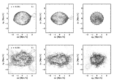
Figure 20: Best fit ellipsoids (solid lines) for halo C1 at $R_{\rm iso}$=$R_{\rm vir}$. The top row shows particles in the equipotential shell, projected to the planes of the ellipsoid (eigenvector coordinate system). The bottom row shows the best fit ellipsoid for the corresponding isodensity range. The dashed circles mark the virial radius. Particles bound to satellites have been removed and remaining particles weighted by their local density prior to fitting.

Figure 21: Ellipsoid fit for the cluster C2.

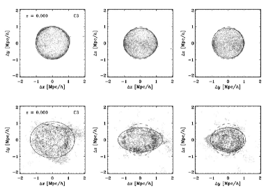
Figure 22: Ellipsoid fit for the cluster C3.

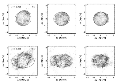
Figure 23: Ellipsoid fit for the cluster C4.

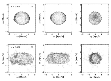
Figure 24: Ellipsoid fit for the cluster C5.

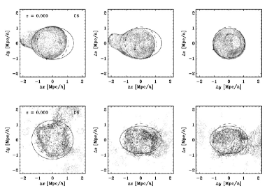
Figure 25: Ellipsoid fit for the cluster C6.

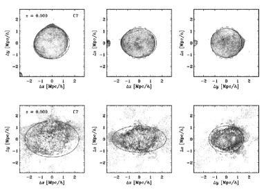
Figure 26: Ellipsoid fit for the cluster C7.

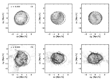
Figure 27: Ellipsoid fit for the cluster C8.

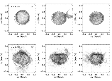
Figure 28: Ellipsoid fit for the galaxy G1.

Appendix D Finding the appropriate tube radius around the orbit

D.1 Iteration

For a given tube radius, we count all particles lying inside the tube around the orbit, thus determining the fraction of ’tube particles’. If more than 68.3% (1 $\sigma$) of the particles are lying inside, the radius is decreased, otherwise enlarged. The procedure is repeated, until we achieve a tube particle fraction of $68.3\%\pm 0.5\%$. If no convergence is reached, we increase the tolerance by a factor of 2, up to 2%. In cases of deviations exceeding 2%, we skip the satellites. This usually is the case, if the number of debris particles is so small, that a meaningful statistic is not possible anymore.

D.2 Particles inside/outside the tube

We check for each particle, whether it lies inside a tube of a given radius or outside.

Instead of first searching for the orbit point closest to the considered particle, we go through the orbit points until one is found, where the particle lies in the tube next to it. Thus, we find one region where the satellite particle lies inside the tube. In fact, there could be more than one suitable region, maybe at some other point the particle would even lie closer to the orbit path. Yet knowing that the particle lies inside the tube at some point is sufficient for our purposes.

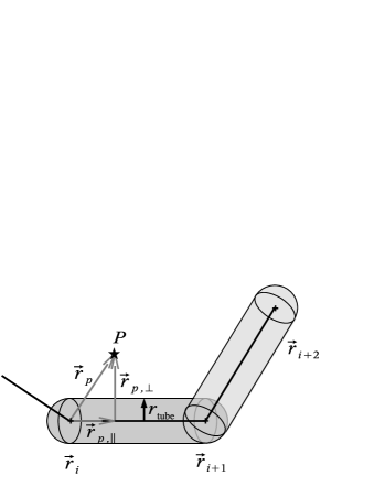
Figure 29: Finding points inside/outside a tube of specified radius $r_{t}$ around the orbit path (thick black line). Not only a cylinder around the orbit path is used, but also the region in a half sphere at the end of each orbit piece is included.

Figure 29 illustrates the situation of particle $P$ lying outside the orbit tube. A particle at distance $\textit{{r}}_{p}$ from an orbit point lies inside the corresponding part of the orbit tube with radius $r_{\rm tube}$, if

• $r_{p,\perp}<r_{\rm tube}$ (within cylinder)

• $r_{p,||}\geq r_{\rm tube}$ (include cap of radius $r_{\rm tube}$ behind the considered orbit point)

• $r_{p,||}\leq|\textit{{r}}_{i+1}-\textit{{r}}_{i}|+r_{\rm tube}$ (not too far beyond next orbit point)

with the orbit points $\textit{{r}}_{i}$ and $\textit{{r}}_{i+1}$ and the components of $\textit{{r}}_{p}$ parallel ($\textit{{r}}_{p,||}$) and perpendicular ($\textit{{r}}_{p,\perp}$) to the orbit path. Particles are not only checked for lying in the cylinder of radius $r_{\rm tube}$ around the orbit path, but also a small half sphere (’cap’) is allowed on front of and behind every orbit point. Otherwise, particles at the kink of the orbit might be wrongly classified as non-tube particles.

References

- Allgood et al. (2006) Allgood B., Flores R. A., Primack J. R., Kravtsov A. V., Wechsler R. H., Faltenbacher A., Bullock J. S., 2006, MNRAS, 367, 1781
- Bailin & Steinmetz (2004) Bailin J., Steinmetz M., 2004, ApJ, 616, 27
- Bailin & Steinmetz (2005) Bailin J., Steinmetz M., 2005, ApJ, 627, 647
- Bullock (2002) Bullock J. S., 2002, in Natarajan P., ed., The shapes of galaxies and their dark halos, Proceedings of the Yale Cosmology Workshop ”The Shapes of Galaxies and Their Dark Matter Halos”, New Haven, Connecticut, USA, 28-30 May 2001. Edited by Priyamvada Natarajan. Singapore: World Scientific, 2002, ISBN 9810248482, p.109 Shapes of dark matter halos. pp 109–+
- Bullock et al. (2001) Bullock J. S., Dekel A., Kolatt T. S., Kravtsov A. V., Klypin A. A., Porciani C., Primack J. R., 2001, ApJ, 555, 240
- Choi et al. (2007) Choi J.-H., Weinberg M. D., Katz N., 2007, ArXiv Astrophysics e-prints
- Davis et al. (1985) Davis M., Efstathiou G., Frenk C. S., White S. D. M., 1985, ApJ, 292, 371
- Diemand et al. (2006) Diemand J., Kuhlen M., Madau P., 2006, ApJ, 649, 1
- Dubinski & Carlberg (1991) Dubinski J., Carlberg R. G., 1991, ApJ, 378, 496
- Franx et al. (1991) Franx M., Illingworth G., de Zeeuw T., 1991, ApJ, 383, 112
- Frenk et al. (1988) Frenk C. S., White S. D. M., Davis M., Efstathiou G., 1988, ApJ, 327, 507
- Gao et al. (2004) Gao L., De Lucia G., White S. D. M., Jenkins A., 2004, MNRAS, 352, L1
- Gao & White (2006) Gao L., White S. D. M., 2006, ArXiv Astrophysics e-prints
- Gao et al. (2004) Gao L., White S. D. M., Jenkins A., Stoehr F., Springel V., 2004, MNRAS, 355, 819
- Gill et al. (2004) Gill S. P. D., Knebe A., Gibson B. K., 2004, MNRAS, 351, 399
- Gill et al. (2005) Gill S. P. D., Knebe A., Gibson B. K., 2005, MNRAS, 356, 1327
- Gill et al. (2004) Gill S. P. D., Knebe A., Gibson B. K., Dopita M. A., 2004, MNRAS, 351, 410
- Hashimoto et al. (2003) Hashimoto Y., Funato Y., Makino J., 2003, ApJ, 582, 196
- Hayashi et al. (2007) Hayashi E., Navarro J. F., Springel V., 2007, MNRAS, 377, 50
- Helmi (2004) Helmi A., 2004, MNRAS, 351, 643
- Hopkins et al. (2005) Hopkins P. F., Bahcall N. A., Bode P., 2005, ApJ, 618, 1
- Ibata et al. (2001) Ibata R., Lewis G. F., Irwin M., Totten E., Quinn T., 2001, ApJ, 551, 294
- Ibata et al. (1994) Ibata R. A., Gilmore G., Irwin M. J., 1994, Nature, 370, 194
- Ibata et al. (2003) Ibata R. A., Irwin M. J., Lewis G. F., Ferguson A. M. N., Tanvir N., 2003, MNRAS, 340, L21
- Ibata et al. (2002) Ibata R. A., Lewis G. F., Irwin M. J., Cambrésy L., 2002, MNRAS, 332, 921
- Jing & Suto (2002) Jing Y. P., Suto Y., 2002, ApJ, 574, 538
- Johnston (1998) Johnston K. V., 1998, ApJ, 495, 297
- Johnston et al. (1996) Johnston K. V., Hernquist L., Bolte M., 1996, ApJ, 465, 278
- Johnston et al. (2005) Johnston K. V., Law D. R., Majewski S. R., 2005, ApJ, 619, 800
- Johnston et al. (2001) Johnston K. V., Sackett P. D., Bullock J. S., 2001, ApJ, 557, 137
- Johnston et al. (2002) Johnston K. V., Spergel D. N., Haydn C., 2002, ApJ, 570, 656
- Johnston et al. (1999) Johnston K. V., Zhao H., Spergel D. N., Hernquist L., 1999, ApJL, 512, L109
- Kasun & Evrard (2005) Kasun S. F., Evrard A. E., 2005, ApJ, 629, 781
- Katz (1991) Katz N., 1991, ApJ, 368, 325
- Kesden & Kamionkowski (2006) Kesden M., Kamionkowski M., 2006, PhRD, 74, 083007
- Knebe et al. (2001) Knebe A., Green A., Binney J., 2001, MNRAS, 325, 845
- Kravtsov et al. (1997) Kravtsov A. V., Klypin A. A., Khokhlov A. M., 1997, ApJS, 111, 73
- Lacey & Cole (1993) Lacey C., Cole S., 1993, MNRAS, 262, 627
- Macciò et al. (2006) Macciò A. V., Dutton A. A., van den Bosch F. C., Moore B., Potter D., Stadel J., 2006, ArXiv Astrophysics e-prints
- McGlynn (1990) McGlynn T. A., 1990, ApJ, 348, 515
- Montuori et al. (2006) Montuori M., Capuzzo-Dolcetta R., Di Matteo P., Lepinette A., Miocchi P., 2006, ArXiv Astrophysics e-prints
- Moore et al. (2004) Moore B., Diemand J., Stadel J., 2004, in Diaferio A., ed., IAU Colloq. 195: Outskirts of Galaxy Clusters: Intense Life in the Suburbs On the age-radius relation and orbital history of cluster galaxies. pp 513–518
- Moore et al. (1999) Moore B., Ghigna S., Governato F., Lake G., Quinn T., Stadel J., Tozzi P., 1999, ApJ, 524, 19L
- Peñarrubia et al. (2006) Peñarrubia J., Benson A. J., Martínez-Delgado D., Rix H. W., 2006, ApJ, 645, 240
- Power (2003) Power C., 2003, Ph.D. Thesis
- Prada et al. (2006) Prada F., Klypin A. A., Simonneau E., Betancort-Rijo J., Patiri S., Gottlöber S., Sanchez-Conde M. A., 2006, ApJ, 645, 1001
- Press et al. (2002) Press W. A., Flannery B. P., Teukolsky S. A., Vetterling W. T., 2002, Numerical Recipes in C: The Art of Scientific Computing, 2nd edition. Cambridge University Press
- Sales et al. (2007) Sales L. V., Navarro J. F., Abadi M. G., Steinmetz M., 2007, MNRAS, 379, 1464
- Springel et al. (2006) Springel V., Frenk C. S., White S. D. M., 2006, Nature, 440, 1137
- Springel et al. (2004) Springel V., White S. D. M., Hernquist L., 2004, in Ryder S., Pisano D., Walker M., Freeman K., eds, IAU Symposium The shapes of simulated dark matter halos. pp 421–+
- Tormen (1997) Tormen G., 1997, MNRAS, 290, 411
- Warnick & Knebe (2006) Warnick K., Knebe A., 2006, MNRAS, 369, 1253
- Warren et al. (1992) Warren M. S., Quinn P. J., Salmon J. K., Zurek W. H., 1992, ApJ, 399, 405