Nonlinear tunneling of BEC in an optical lattice: signatures of quantum collapse and revival

Abstract

Quantum theory of the intra-band resonant tunneling of a Bose-Einstein condensate loaded in a two-dimensional optical lattice is considered. It is shown that the phenomena of quantum collapse and revival can be observed in the fully quantum problem. The meanfield limit of the theory is analyzed using the WKB approximation for discrete equations, establishing in this way a direct connection between the two approaches conventionally used in very different physical contexts. More specifically we show that there exist two different regimes of tunneling and study dependence of quantum collapse and revival on the number of condensed atoms.

I Introduction

Passage from the exact many-body description of an atomic gas at zero temperature to the mean-field theory is based on the assumption about large occupation number $N$ of the ground (or, more generally, some specific quantum) state. Then $N^{-1/2}$ can be shown to be the parameter of expansion, which in the leading order gives the Gross-Pitaevskii equation Gardiner . Respectively, the mentioned requirement must be also applied to mean-field theories of the Landau-Zener tunneling Landau-Zener ; KKS ; SHCH , for which interesting experimental data are available experiment , to instabilities of BEC’s in optical lattices KKS ; instabil observed experimentally in instb-experim , and to a theory of nonlinear Bloch–band tunneling BKK . Similar approach was also exploited in a pure quantum theory of a Bose-Einstein condensate (BEC) in a double-well trap JM , based on a model with linear coupling JZM . Either for the Bloch–band tunneling problem or for the tunneling in a double-well potential the approach of large $N$ is justified when the system is close to the mean-field regime and the respective dynamical solutions are characterized by the essentially nonzero populations of the quantum states between which tunneling occurs. Such regimes indeed exist when the description is reduced to a dimer RSFS . At the same time the mean-field approximation to the above problems allows solutions where the populations of the states repeatedly become zero. Strictly speaking this violates the initially made supposition about large atomic numbers, because a state with negligible population cannot be treated in the mean-filed approximation. Therefore the theory requires modifications.

We thus can formulate the main goal of the present paper as the analysis of the macroscopic nonlinear tunneling between two quantum states with the same (or infinitely close) energies in the limit corresponding to large total number of particles, allowing however populations of each of the states to become negligibly small at some moments of time. We will pay the main attention to the quantum effects, not accounted by the standard mean-field theory.

To be specific, as a physical system we explore a BEC loaded in a two-dimensional optical lattice and consider tunneling between two states with the same energy. Such a situation can be experimentally realized in at least two different ways. First, one can use a non-separable lattice, with properly chosen parameters providing closer of the lowest gap (as, for example, this is suggested in BKK ). Then nonlinear tunneling occurs between X and M points of two different bands (see Fig. 1). More general situation, however, corresponds to the nonlinear tunneling between two X points of the same band, rotated by $\pi/2$ with respect to each other (these are the points X_1,2 in Fig. 1). Such intra–band tunneling does not depend on the size of the gap, and hence can be observed in any lattice including separable one. Moreover, whenever one deals with the nonlinear tunneling, the stability issue acquires especial importance KKS ; BKK , since depending on the sign of the effective mass the homogeneous excitations can be either modulationally stable or unstable. This in particular means that tunneling between two states in different bands (like tunneling between X and M points, mentioned above, or, tunneling in one-dimensional case between two neighbor zones) represents a transition between stable and unstable states, what causes asymmetry of the tunneling. That is why, in the present paper we concentrate on intra–band tunneling between two stable X points, what rules out instability and allows one to limit the consideration to plane Bloch waves.

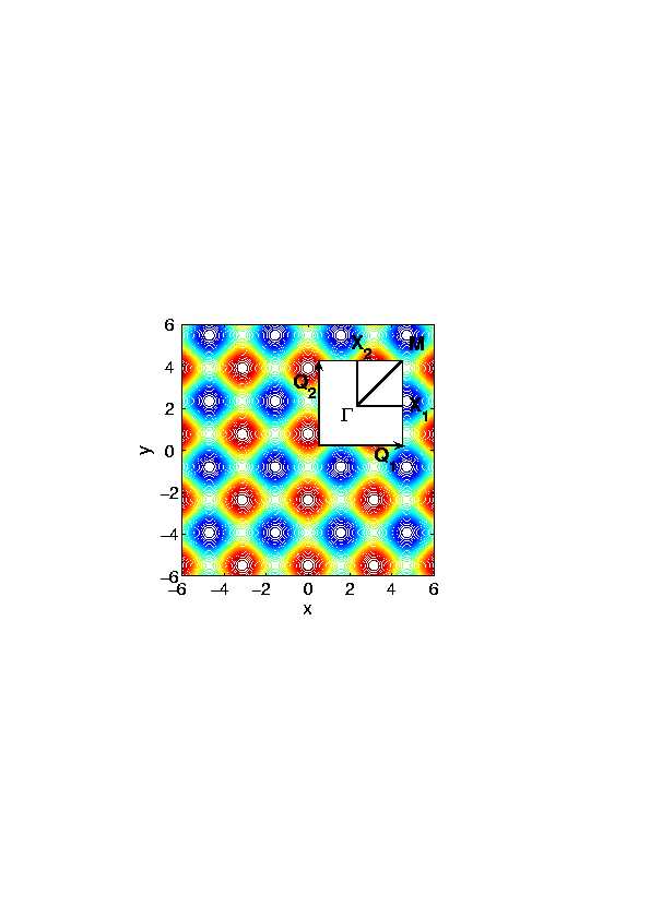
Figure 1: (Color online) The contour plot of the periodic potential, given by equation (38) below, used for the numerical simulations. The inset shows the first Brillouin zone, the reciprocal lattice basis vectors ${\bf Q}_{1,2}$ and the high symmetry points $\Gamma$, M, and X_j. The nonlinear intra-band tunneling occurs between the points X₁ and X₂.

In the mean-field approximation this problem was considered in BKKS , which in the two-mode approximation is reduced to a model imitating either a Josephson junction or Rabi oscillations in a system of two-level atoms. Such a model describes population oscillations between two states. Using the mentioned analogy, one can predict that quantization of the motion should result in quantum collapse and revival of the above oscillations CBPZ . Obtaining those phenomena in the process of intra-band tunneling, constitutes the second aim of the present paper.

Finally, we emphasize an interesting mathematical aspect of the problem at hand. Namely, we will establish a formal link between the mean-field approximation, where the small parameter can be identified as $1/N$ and the discrete WKB method, having $\hbar$ as a formal small parameter, which is described in details in Ref. braun . In our approach the both methods, appearing originally as independent as they are used in different setups and based on different physical assumptions, are intimately related to each other allowing us to appreciate the accuracy of the mean-field model, what will be the third goal of the present work. It is to be mentioned that earlier the link between the semi-classical and mean-field approaches was discussed in VA , where a linearly couped two-level system, modeling either a BEC in a double-well trap or a spinor condensate, was considered and where the quantum corrections appeared as a decoherence of the quantum states. We, thus present one more physical system, a BEC in an optical lattice, having no linear coupling and rather different stability properties, which also allows experimental verification of the mean-field approximation. In our case the quantum effects will be manifested through the quantum collapse.

The paper is organized as follows. In Sec. II we deduce the quantum two-mode model describing resonant intra-band tunneling, expand its solution over the Fock basis and deduce the dynamical system for the expansion coefficients. In Sec. III we discuss the mean-field approximation starting with the derived dynamical system and based on the WKB method for discrete equations. Sec. IV is devoted to numerical study of the both, full quantum and mean-field models. The outcomes are summarized in the Conclusion.

II Quantum model

II.1 Inter– and intra– band transitions

Let us start with the Hamiltonian of a BEC in a two-dimensional, ${\bf x}\in\mathbb{R}^{2}$, optical lattice $V({\bf x})$,

$$H=\int\limits_{\mathcal{V}}\mathrm{d}^{2}{\bf x}\psi^{\dagger}({\bf x})\left(-\frac{\hbar^{2}}{2m}\nabla^{2}+V({\bf x})\right)\psi({\bf x})$$

$$+\frac{g}{2}\int\limits_{\mathcal{V}}\mathrm{d}^{2}{\bf x}\psi^{\dagger}({\bf x})\psi^{\dagger}({\bf x})\psi({\bf x})\psi({\bf x}),$$ (1)

where $\mathcal{V}=Mv_{0}$ is the total area of the lattice consisting of $M$ cells each one of the area $v_{0}$, $g$ is the interaction coefficient in two dimensions, and $\psi^{\dagger}({\bf x})$ and $\psi({\bf x})$ are the creation and annihilation field operators. Introducing the Bloch waves $\varphi_{n{\bf k}}({\bf x})$ through the standard eigenvalue problem $\left(-\frac{\hbar^{2}}{2m}\nabla^{2}+V({\bf x})\right)\varphi_{n{\bf k}}=E_{n{\bf k}}\varphi_{n{\bf k}}$, where $n$ is a number of the zone and ${\bf k}$ is the wave-vector in the first Brillouin zone (BZ), and considering them orthonormalized, $\int_{\mathcal{V}}\bar{\varphi}_{n{\bf k}}({\bf x})\varphi_{n^{\prime}{\bf k}^{\prime}}({\bf x})d{\bf x}=\delta_{nn^{\prime}}\delta_{{\bf k}{\bf k}^{\prime}}$, we represent

$$\psi({\bf x})=\sum_{n,{\bf k}}\varphi_{n,{\bf k}}({\bf x})b_{n,{\bf k}},$$ (2)

where the creation and annihilation operators satisfy the usual commutation relations $[b_{n{\bf k}},b_{n^{\prime}{\bf k}^{\prime}}]=0$ and $[b_{n{\bf k}},b^{\dagger}_{n^{\prime}{\bf k}^{\prime}}]=\delta_{nn^{\prime}}\delta_{{\bf k}{\bf k}^{\prime}}$.

The expansion (2) allows one to rewrite the Hamiltonian in the form

$$H=\sum_{n,{\bf k}}E_{n{\bf k}}b^{\dagger}_{n{\bf k}}b_{n{\bf k}}+$$

$$\sum_{{\bf k}_{1},...,{\bf k}_{4}\atop n_{1},...,n_{4}}\chi^{n_{1}n_{2}n_{3}n_{4}}_{{\bf k}_{1}{\bf k}_{2}{\bf k}_{3}{\bf k}_{4}}\delta_{{\bf k}_{1}+{\bf k}_{2}-{\bf k}_{3}-{\bf k}_{4},{\bf Q}}b^{\dagger}_{n_{1}{\bf k}_{1}}b^{\dagger}_{n_{2}{\bf k}_{2}}b_{n_{3}{\bf k}_{3}}b_{n_{4}{\bf k}_{4}},$$

(3)

where ${\bf Q}$ is an arbitrary vector of the reciprocal lattice,

$$\chi^{n_{1}n_{2}n_{3}n_{4}}_{{\bf k}_{1}{\bf k}_{2}{\bf k}_{3}{\bf k}_{4}}=\frac{g}{2}\int\limits_{\mathcal{V}}\mathrm{d}^{2}{\bf x}\varphi^{*}_{n_{1}{\bf k}_{1}}\varphi^{*}_{n_{2}{\bf k}_{2}}\varphi_{n_{3}{\bf k}_{3}}\varphi_{n_{4}{\bf k}_{4}}$$ (4)

(hereafter an asterisk stands for complex conjugation).

Next we apply the rotating wave approximation, i.e. neglect all four-wave processes which do not satisfy the energy conservation law. This allows us to simplify the Hamiltonian (3):

$$H=\sum_{n,{\bf k}}E_{n{\bf k}}b^{\dagger}_{n{\bf k}}b_{n{\bf k}}+$$

$$\sum_{{\bf k}_{1},...,{\bf k}_{4}\atop n_{1},...,n_{4}}\delta_{{\bf k}_{1}+{\bf k}_{2},{\bf k}_{3}+{\bf k}_{4}+{\bf Q}}\delta_{E_{n_{1}{\bf k}_{1}}+E_{n_{2}{\bf k}_{2}},E_{n_{3}{\bf k}_{3}}+E_{n_{4}{\bf k}_{4}}}$$

$$\times\chi^{n_{1}n_{2}n_{3}n_{4}}_{{\bf k}_{1}{\bf k}_{2}{\bf k}_{3}{\bf k}_{4}}b^{\dagger}_{n_{1}{\bf k}_{1}}b^{\dagger}_{n_{2}{\bf k}_{2}}b_{n_{3}{\bf k}_{3}}b_{n_{4}{\bf k}_{4}}.$$ (5)

Further reduction of the Hamiltonian can be done by taking into account that the periodic medium is highly dispersive, and therefore for the resonant four-wave interactions, equality of the group velocities of the respective matter waves must be imposed. In the case of tunneling between two states, say $(n_{1},{\bf q}_{1})$ and $(n_{2},{\bf q}_{2})$, this means the constraint $\partial E_{n_{1}{\bf q}_{1}}/\partial{\bf q}_{1}=\partial E_{n_{2}{\bf q}_{2}}/\partial{\bf q}_{2}$. Together with the momentum and energy conservation laws, expressed by the first and the second Kronecker deltas in (5), this means that the resonant nonlinear tunneling can occur only between highly symmetric points of the BZ. As far as we have limited ourselves to the intra-band tunneling, we conclude that the only points of the BZ – the points X – satisfies the above requirements. Moreover, in the BZ there are only two physically different X-points. Assuming that the lattice is orthogonal with a period $d$ in the both directions, the BZ can be identified simply as the domain $[-\frac{\pi}{d},\frac{\pi}{d}]\times[-\frac{\pi}{d},\frac{\pi}{d}]$. Consequently the two X-points we are interested in, below they are referred to as X₁ and X₂, correspond to the two vectors ${\bf q}_{1}=\left(0,\frac{\pi}{d}\right)$ and ${\bf q}_{2}=\left(\frac{\pi}{d},0\right)$. The group velocities in these points are zero.

Now one readily verifies that (5) is significantly simplified allowing one to rewrite the Hamiltonian in the form of a sum

$$H=\sum_{n}H_{n}+H_{i-b}$$ (6)

where

$$H_{n}=E_{n{\bf q}_{1}}b^{\dagger}_{n{\bf q}_{1}}b_{n{\bf q}_{1}}+E_{n{\bf q}_{2}}b^{\dagger}_{n{\bf q}_{2}}b_{n{\bf q}_{2}}+\chi_{{\bf q}_{1}{\bf q}_{1}}^{nn}\left(b^{\dagger}_{n{\bf q}_{1}}b^{\dagger}_{n{\bf q}_{1}}b_{n{\bf q}_{1}}b_{n{\bf q}_{1}}+b^{\dagger}_{n{\bf q}_{2}}b^{\dagger}_{n{\bf q}_{2}}b_{n{\bf q}_{2}}b_{n{\bf q}_{2}}\right)$$

$$+\chi_{{\bf q}_{1}{\bf q}_{2}}^{nn}\left(b^{\dagger}_{n{\bf q}_{1}}b^{\dagger}_{n{\bf q}_{1}}b_{n{\bf q}_{2}}b_{n{\bf q}_{2}}+b^{\dagger}_{n{\bf q}_{2}}b^{\dagger}_{n{\bf q}_{2}}b_{n{\bf q}_{1}}b_{n{\bf q}_{1}}+4b^{\dagger}_{n{\bf q}_{1}}b^{\dagger}_{n{\bf q}_{2}}b_{n{\bf q}_{1}}b_{n{\bf q}_{2}}\right)$$ (7)

describes intra-band transitions between states X₁ and X₂ of the $n$-th band and

$$H_{i-b}=4\sum_{n_{1}n_{2}\atop n_{1}\neq n_{2}}\chi^{n_{1}n_{2}}_{{\bf q}_{1}{\bf q}_{2}}\left(b^{\dagger}_{n_{1}{\bf q}_{1}}b^{\dagger}_{n_{2}{\bf q}_{2}}+b^{\dagger}_{n_{2}{\bf q}_{1}}b^{\dagger}_{n_{1}{\bf q}_{2}}\right)\left(b_{n_{1}{\bf q}_{1}}b_{n_{2}{\bf q}_{2}}+b_{n_{2}{\bf q}_{1}}b_{n_{1}{\bf q}_{2}}\right)$$ (8)

describes transitions between X points of different bands. In the above formulas we introduced $\chi^{n_{1}n_{2}}_{{\bf q}_{1}{\bf q}_{2}}=\chi_{{\bf k}_{1}{\bf k}_{2}{\bf k}_{1}{\bf k}_{2}}^{n_{1}n_{2}n_{1}n_{2}}$ and used the symmetry properties of the Bloch functions, giving in particular $\chi_{{\bf q}_{1}{\bf q}_{1}}^{nn}=\chi_{{\bf q}_{2}{\bf q}_{2}}^{nn}$ and $\chi_{{\bf q}_{1}{\bf q}_{2}}^{nn}=\chi_{{\bf q}_{2}{\bf q}_{1}}^{nn}$, as well as the fact that $\varphi_{n{\bf q}_{1}}$ and $\varphi_{n{\bf q}_{2}}$ correspond to X points and hence can be chosen real and periodic.

II.2 Dynamical equations and their accuracy

Dynamics of the condensate can be described by the time evolution of the coefficients of the expansion of a given multiparticle state $|\Psi(t)\rangle$ over the Fock basis. In the case when initially one band, say the band $n_{0}$, is populated more densely than the other ones, it is natural to represent the basis as $|N_{1},N_{2};{\bf n}\rangle$, where $N_{j}$ stand for the occupation numbers of the states ${\rm X}_{j}$ of the given band, while ${\bf n}$ symbolically designate occupation numbers of all other bands. Thus

$$|\Psi(t)\rangle=\sum_{N_{1},N_{2},{\bf n}}C_{N_{1}N_{2}{\bf n}}(t)|N_{1},N_{2};{\bf n}\rangle$$ (9)

Now we consider the situation, where initially (i.e. at $t=0$) all atoms belong to X points of the chosen band, i.e. when $N_{1}+N_{2}=N$ with $N$ being the total number of particles. Then, introducing the simplified notation $|N_{1},N_{2}\rangle=|N_{1},N_{2};{\bf 0}\rangle$ for such states, which also can be rewritten as $|N_{1},N_{2}\rangle=|k,N-k\rangle=|k\rangle|N-k\rangle$ (here $k=N_{1}$), and respectively $C_{N_{1}N_{2}0}(t)\equiv C_{k}(t)$, we can express

$$|\Psi(0)\rangle=\sum_{k=0}^{N}C_{k}(0)|k,N-k\rangle,\quad\sum_{k=0}^{N}|C_{k}(0)|^{2}=1.$$ (10)

For the next step, it is not difficult to verify that the dynamics of a state, initially spanned over the kets $|k,N-k\rangle$, i.e. subject to the initial condition (10), which is induced by the Hamiltonian (6) results only in the states belonging to initial sub-space, i.e.

$$|\Psi(t)\rangle=\sum_{k=0}^{N}C_{k}(t)|k,N-k\rangle,\quad\sum_{k=0}^{N}|C_{k}(t)|^{2}=1.$$ (11)

for all $t$.

Indeed, substituting (9) in the Shrödinger equation

$$i\frac{\partial|\Psi\rangle}{\partial t}=H|\Psi\rangle$$ (12)

and applying $\langle N_{1},N_{2};{\bf n}|$ in order to obtain the equations for the expansion coefficients, one finds that for all coefficients with $N_{1}+N_{2}<N$ (i.e. for states with ${\bf n}\neq 0$) the derivatives $dC_{N_{1}N_{2}{\bf n}}/dt$ linearly depend on different $C_{N_{1}^{\prime}N_{2}^{\prime}{\bf n}^{\prime}}$ with $N_{1}^{\prime}+N_{2}^{\prime}<N$, but do not depend on $C_{N_{1}N_{2}0}$. This follows from the relations $H_{i-b}|N_{1},N_{2}\rangle=0$ and $H_{n}|N_{1},N_{2}\rangle=0$ for $n\neq n_{0}$. The first of these formulas means that no coupling occurs when at least one of the states in not occupied, while the second relation means zero result when one probes the energy of an empty band ($H_{n}$ does not originate inter-band transitions) and in our case the only band, $n_{0}=0$, is initially occupied. Thus all the coefficients $C_{N_{1}N_{2}{\bf n}}$ with ${\bf n}\neq 0$ are identically equal to zero, provided they are zero at $t=0$.

Summarizing the described situation subject to assumption that only one band $n_{0}$ is populated and neglecting the unessential for the dynamics linear energy term $E_{n_{0}{\bf q}_{1}}+E_{n_{0}{\bf q}_{2}}$, one arrives at the two-mode model whose Hamiltonian can be written down in the form

$$H_{n_{0}}=H_{0}-E_{n_{0}{\bf q}_{1}}-E_{n_{0}{\bf q}_{2}}$$

$$=\chi_{11}\left\{n_{1}^{2}+n_{2}^{2}+\Lambda\left[4n_{1}n_{2}+(b_{1}^{\dagger})^{2}b_{2}^{2}+(b_{2}^{\dagger})^{2}b_{1}^{2}\right]\right\},$$

(13)

where $b_{j}=b_{n_{0}{\bf q}_{j}}$, i.e. $b^{\dagger}_{1}|k,N-k\rangle=\sqrt{k+1}|k+1,N-k\rangle$ and $b^{\dagger}_{2}|k,N-k\rangle=\sqrt{N-k+1}|k,N-k+1\rangle$, $n_{j}=b^{\dagger}_{n_{0}{\bf q}_{j}}b_{n_{0}{\bf q}_{j}}$ are the populations of the states $X_{j}$ of the band $n_{0}$, $\chi_{11}=\chi_{q_{1}q_{1}}^{n_{0}n_{0}}$, and $\Lambda=\chi_{{\bf q}_{1}{\bf q}_{2}}^{n_{0}n_{0}}/\chi_{{\bf q}_{1}{\bf q}_{1}}^{n_{0}n_{0}}$. Hamiltonian (13) preserves the total number of atoms in the $X_{j}$-points, what naturally reflects the approximations made.

The above calculations, which resulted in (13), hold for the more general Hamiltonian (5) obtained in the rotating wave approximation, but fail for the original model accounting all possible transitions (not only the resonant ones). This defines the accuracy of the two-mode approximation: the ratios between the accounted and neglected terms are of the order of $1/N$.

Now the Schrödinger equation (12) with $H=H_{0}$ results in a system of ordinary differential equations for the coefficients $C_{k}$

$$\frac{i}{N}\frac{\mathrm{d}C_{k}}{\mathrm{d}\tau}=\frac{\Lambda}{4}(b_{k-1}C_{k-2}+b_{k+1}C_{k+2})+\frac{a_{k}}{4}C_{k},$$ (14)

with the dimensionless time $\tau=(4\chi_{11}N/\hbar)t$ and with the coefficients

$$a_{k}=1+2(2\Lambda-1)\frac{k}{N}\left(1-\frac{k}{N}\right),$$ (15)

$$b_{k}=\left[\frac{k}{N}\left(\frac{k}{N}+\frac{1}{N}\right)\left(1-\frac{k}{N}\right)\left(1-\frac{k}{N}+\frac{1}{N}\right)\right]^{\frac{1}{2}}.$$ (16)

III Fictitious particle representation and the semiclassical limit

III.1 Mean-field equations viewed as a quasi-classical limit.

Equation (14) can be viewed as the Schrödinger equation for a fictitious quantum particle in the one-dimensional discrete space $k=\{0,1,2,\ldots,N\}$. Indeed, setting $x=k/N$ and $h=2/N$, introducing a differentiable function $\psi(x)$ of the continuous variable $x\in(0,1)$, such that $\psi(x)=\sqrt{N}C_{k}$ at the points $x=k/N$  let us define the quantities:

$$b^{(\pm)}_{h}(x)=b_{h}(x+h/2)\pm b_{h}(x-h/2),$$

$$b_{h}(x)=[x(x+h/2)(1-x)(1-x+h/2)]^{1/2},$$

$$a(x)=1+2(2\Lambda-1)b_{0}(x).$$

Now equation (14) becomes

$$ih\partial_{\tau}\psi(x)=\frac{a(x)}{2}\psi(x)$$

$$+\frac{\Lambda}{2}\left\{b_{h}\left(x+\frac{h}{2}\right)e^{i\hat{p}}+b_{h}\left(x-\frac{h}{2}\right)e^{-i\hat{p}}\right\}\psi(x).$$

(17)

Here the parameter $h$ plays the role of the Plank constant $\hbar$, $\hat{p}\equiv-ih\partial_{x}$ is the “momentum operator” of the fictitious particle, and the “wave function” $\psi(x)$ is assumed to be normalized in the usual way $\int_{0}^{1}\mathrm{d}x|\psi(x)|^{2}=1$.

Equation (17) describes a fictitious quantum particle of the mass proportional to $1/\Lambda$ moving in a compact curved space defined by the interval $(0,1)$ (hence $b^{(\pm)}_{h}(x)$ at the functions of the momentum operator). Note that the “momentum” eigenvalues can be restricted to the first BZ, i.e. $[-\frac{\pi}{d},\frac{\pi}{d}]$.

The semiclassical dynamics corresponds to the limit $h\to 0$, i.e. when the number of BEC atoms $N\to\infty$, what is the usual limit of the Gross-Pitaevskii equation. It should be noted that the characteristic time $t$ of the evolution scales as $(gN)^{-1}\tau$, hence the quantity $gN$ must be kept fixed, which is the second condition of the mean-field limit. It is also clear that the limit $h\to 0$, if it exists, corresponds to the continuous limit of the discrete equation (17) (see also Ref. braun ).

In order to derive the quasi-classical equation corresponding to the limit $h\to 0$ we proceed in the usual way. Setting $\psi(x,\tau)=e^{iS(x,\tau,h)/h}$ for a complex action $S(x,\tau,h)$ viewed as a series $S=S^{(0)}+hS^{(1)}+\ldots$, we get the equation

$$-S_{\tau}=\frac{\Lambda}{2}\left\{b_{h}\left(x+\frac{h}{2}\right)e^{i\frac{S(x+h)-S(x)}{h}}+b_{h}\left(x-\frac{h}{2}\right)e^{i\frac{S(x-h)-S(x)}{h}}\right\}+\frac{a(x)}{2}.$$ (18)

Assuming that the function $S(x,\tau,h)$ has derivatives with respect to $x$ up to the second order, expanding

$$\frac{S(x\pm h)-S(x)}{h}=\pm S^{(0)}_{x}+\mathcal{O}(h)$$

and setting $h\to 0$ in the equation (18) we get the Hamilton-Jacobi equation for the classical action $\tilde{S}(x,\tau)=S^{(0)}(x,\tau)-\tau/2$:

$$-\tilde{S}_{\tau}=b_{0}(x)\left\{\Lambda\cos(\tilde{S}_{x})+2\Lambda-1\right\}$$ (19)

[recall that $b_{0}(x)=x(1-x)$].

Thus the physical sense of the transition to the classical limit in our problem is the transition from a discrete equation to its continuous limit. Note that in our setup the usual classical limit $\hbar\to 0$, sometimes understood as a mathematical abstraction, acquires the well established sense of the limit of a large number of atoms and thus can be studied experimentally.

In the case of a finite $h$ (finite $N$) we have $[\hat{p},x]=-ih$, i.e. the usual canonical commutator of the momentum and coordinate. It turns out, however, that quasi-classical dynamics is more convenient to describe in terms of variables $z=1-2x$ and $\Phi=\tilde{S}_{x}=p$, where $x$ and $p$ are the classical limits of the corresponding quantum variables. Then the Poisson brackets of the respective classical dynamics read

$$\{\Phi,z\}=\lim_{h\to 0}\frac{i}{h}[\hat{p},1-2x]=-2.$$

and the classical Hamiltonian can be recovered from the Hamilton-Jacobi equation (19):

$$\mathcal{H}=\frac{1}{4}(1-z^{2})(2\Lambda+\Lambda\cos\Phi-1).$$ (20)

Thus the classical Hamiltonian equations have the form

$$\dot{z} = -2\frac{\partial H}{\partial\Phi}=\frac{\Lambda}{2}(1-z^{2})\sin\Phi,$$ (21a)

$$\dot{\Phi} = 2\frac{\partial H}{\partial z}=(1-2\Lambda-\Lambda\cos\Phi)z.$$ (21b)

In our case these equations correspond to the mean field approximation.

In order to clarify the physical meaning of the introduced classical variables $z$ and $\Phi$ let us compute

$$\langle\Psi|(n_{2}-n_{1})|\Psi\rangle=N\sum_{N_{1},N_{2}\atop N_{1}+N_{2}=N}C_{N_{1}}^{*}\frac{N_{2}-N_{1}}{N}C_{N_{1}}$$

$$=N\left(1-2\sum_{k=0}^{N}\frac{k}{N}|C_{k}|^{2}\right)=N(1-2\langle x\rangle),$$ (22)

and

$$\langle\Psi|(b_{2}^{\dagger})^{2}b_{1}^{2}|\Psi\rangle=N^{2}\sum_{k=0}^{N}C_{k}^{*}b_{k+1}C_{k+2}$$

$$=N^{2}\langle b_{h}\left(x+\frac{h}{2}\right)e^{i\hat{p}}\rangle$$ (23)

(in the last formula we used that $C_{k+2}=e^{i\hat{p}}C_{k}$).

Thus in the limit $h\to 0$

$$z=\lim_{h\to 0}\langle z\rangle=\frac{\langle n_{2}\rangle-\langle n_{1}\rangle}{N}$$ (24)

is the relative population of the states (as it is clear $z\in[-1,1]$) and

$$\Phi=\lim_{h\to 0}\langle\hat{p}\rangle=\mathrm{arg}\langle(b_{2}^{\dagger})^{2}b_{1}^{2}\rangle.$$ (25)

is the relative phase.

III.2 On the mean-field dynamics

Let us now discuss some aspects of the dynamics described by the mean-field approximation. First of all we observe that the system (21) has two fixed points: $P_{1}=(z=0,\Phi=0)$ and $P_{2}=(z=0,\Phi=\pi)$. The respective frequencies are $\Omega^{2}_{1}=\frac{3\Lambda}{2}(\Lambda-\Lambda_{c})$ and $\Omega^{2}_{2}=\frac{\Lambda}{2}(1-\Lambda)$ with $\Lambda_{c}=1/3$. Thus one easily verifies that $P_{2}$ is a local maximum, while $P_{1}$ is a saddle-point for $\Lambda<\Lambda_{c}$ and a local minimum for $\Lambda>\Lambda_{c}$.

Next, following Ref. braun we take into account that the classical energy $E={\cal H}(z,\Phi)$ is bounded by the two potential curves, one corresponding to $\Phi=0$ [the curve $U^{(+)}(x)$] and the other to $\Phi=\pi$ [the curve $U^{(-)}(x)]$:

$$U^{(-)}(x)=(\Lambda-1)b_{0}(x),\;U^{(+)}(x)=(3\Lambda-1)b_{0}(x),$$ (26)

i.e. $U^{(-)}(x)\leq E\leq U^{(+)}(x)$. Therefore, the turning points of the classical system (21a)-(21b) lie on the curves $U^{(\pm)}(x)$. One can express the period of oscillations between two turning points $x_{1}$ and $x_{2}$ as follows

$$T=2\int\limits_{x_{1}}^{x_{2}}\frac{\mathrm{d}x}{\sqrt{(U^{(+)}-E)(E-U^{(-)})}}.$$ (27)

This integral can be expressed in terms of the complete elliptic integral of the first kind $K(\cdot)$. To this end we single out four physically different cases:

Case 1: If $\Lambda<\Lambda_{c}$ and the energy of “classical” motion is $(3\Lambda-1)/4<E<0$, the turning points belong to different curves, for instance:

$$x_{1}=\frac{1}{2}\left(1-\sqrt{1+\frac{4E}{1-\Lambda}}\right)\in U^{(-)}$$

$$x_{2}=\frac{1}{2}\left(1-\sqrt{1+\frac{4E}{1-3\Lambda}}\right)\in U^{(+)}$$

and the period is given by

$$\displaystyle{T_{1}=\frac{4K\left(\frac{2\sqrt{-2E\Lambda}}{\sqrt{(1-3\Lambda)(1-\Lambda+4E)}}\right)}{\sqrt{(1-3\Lambda)(1-\Lambda+4E)}}\,.}$$ (28)

The difference in the atomic population oscillates about a nonzero value.

Case 2: If $\Lambda<\Lambda_{c}$ and the energy of “classical” motion is $(\Lambda-1)/4<E<(3\Lambda-1)/4<0$, the turning points belong to a single curve:

$$x_{1,2}=\frac{1}{2}\left(1\pm\sqrt{1+\frac{4E}{1-\Lambda}}\right)\in U^{(-)}$$

and the period is given by

$$\displaystyle{T_{2}=\frac{2\sqrt{2}}{\sqrt{-\Lambda E}}K\left(\frac{\sqrt{(1-3\Lambda)(1-\Lambda+4E)}}{2\sqrt{-2E\Lambda}}\right)\,.}$$ (29)

The difference in the atomic population oscillates about zero.

Case 3: If $\Lambda>\Lambda_{c}$ and the energy of “classical” motion is in the interval $(\Lambda-1)/4<E<0$, the turning points belong to a single curve:

$$x_{1,2}=\frac{1}{2}\left(1\pm\sqrt{1+\frac{4E}{1-\Lambda}}\right)\in U^{(-)}$$

and the period is given by

$$\displaystyle{T_{3}=\frac{8K\left(\sqrt{\frac{1+\frac{4E}{1-\Lambda}}{1+\frac{4E}{1-3\Lambda}}}\right)}{\sqrt{(1-\Lambda)(3\Lambda-1-4E)}}\,.}$$ (30)

The two states have equal average populations.

Case 4: If $\Lambda>\Lambda_{c}$ and the energy of “classical” motion is in the interval $0<E<(3\Lambda-1)/4$, the turning points belong to a single curve:

$$x_{1,2}=\frac{1}{2}\left(1\pm\sqrt{1+\frac{4E}{1-3\Lambda}}\right)\in U^{(+)}$$

and the period is given by

$$\displaystyle{T_{4}=\frac{8K\left(\sqrt{\frac{1+\frac{4E}{1-3\Lambda}}{1+\frac{4E}{1-\Lambda}}}\right)}{\sqrt{(3\Lambda-1)(1-\Lambda-4E)}}\,.}$$ (31)

The two states have equal average populations.

Finally we mention that equations (21) can be directly obtained from the two-mode Hamiltonian of the Bloch-band tunneling in the meanfield approximation (see BKKS ; comm1 for more details):

$$H_{m-f}=\chi_{11}|{\cal A}_{1}|^{4}+\chi_{11}|{\cal A}_{2}|^{4}+4\chi_{12}|{\cal A}_{1}|^{2}|{\cal A}_{2}|^{2}$$

$$+\chi_{12}({\cal A}_{1}^{*})^{2}{\cal A}_{2}^{2}+\chi_{12}({\cal A}_{2}^{*})^{2}{\cal A}_{1}^{2}\,.$$ (32)

where the complex amplitudes ${\cal A}_{1,2}$ are determined by the expansion of the order parameter $\Psi$

$$\Psi={\cal A}_{1}(t)\varphi_{1}({\bf r})e^{-iEt}+{\cal A}_{2}(t)\varphi_{2}({\bf r})e^{-iEt}\,$$ (33)

and determine average populations of the levels ${\cal N}_{j}=|{\cal A}_{j}|^{2}$, and $\varphi_{j}({\bf r})$ are the respective Bloch states. The complex amplitudes are connected by the particle conservation law: $N={\cal N}_{1}+{\cal N}_{2}$. Now the system (21a), (21b) is obtained from the Hamiltonian equations by defining

$$z=\frac{|{\cal A}_{2}|^{2}-|{\cal A}_{1}|^{2}}{{\cal N}}\quad\mbox{and}\quad\Phi=\arg\{{\cal A}_{1}^{2}({\cal A}_{2}^{*})^{2}\}$$ (34)

[c.f. Eq. (25)].

III.3 “Coherent” states

Turning now to the quantum system, we observe that the dynamical equations for the coefficients $C_{n}$ have to be supplied by the initial conditions. As in the standard WKB approximation, the corresponding initial conditions must be smooth enough. At the same time a natural question arises about construction of quantum states, $|\Psi(t)\rangle_{c}$, most closely resembling the meanfield dynamics. We will refer to such states as coherent states.

In order to construct such states we recall the explicit form of the meanfield ansatz (33) and consider the respective boson operator $c^{\dagger}=\alpha_{1}b^{\dagger}_{1}+\alpha_{2}b^{\dagger}_{2}$, where $\alpha_{1,2}$ are time dependent complex parameters satisfying $|\alpha_{1}|^{2}+|\alpha_{2}|^{2}=1$. Next we define

$$|\Psi(t)\rangle_{c} \equiv |\alpha_{1},\alpha_{2}\rangle\equiv\frac{(\alpha_{1}(t)b^{\dagger}_{1}+\alpha_{2}(\textbf{}t)b^{\dagger}_{2})^{N}}{\sqrt{N!}}|0,0\rangle$$ (35)

$$= \sum_{k=0}^{N}\sqrt{\frac{N!}{k!(N-k)!}}\alpha_{1}^{k}\alpha_{2}^{N-k}|k,N-k\rangle.$$

By using the identities:

$$\langle\alpha_{1},\alpha_{2}|n_{j}|\alpha_{1},\alpha_{2}\rangle=N|\alpha_{j}|^{2},$$

$$\langle\alpha_{1},\alpha_{2}|n_{j}^{2}|\alpha_{1},\alpha_{2}\rangle=N|\alpha_{j}|^{2}+N(N-1)|\alpha_{j}|^{4},$$

$$\langle\alpha_{1},\alpha_{2}|n_{1}n_{2}|\alpha_{1},\alpha_{2}\rangle=N(N-1)|\alpha_{1}\alpha_{2}|^{2},$$

$$\langle\alpha_{1},\alpha_{2}|(b_{2}^{\dagger})^{2}b_{1}^{2}|\alpha_{1},\alpha_{2}\rangle=N(N-1)\alpha_{1}^{2}(\alpha_{2}^{*})^{2},$$

we obtain for the energy (dropping an inessential constant)

$$E=\langle\alpha|H|\alpha\rangle=\chi_{11}N(N-1)$$

$$\times\left\{|\alpha_{1}|^{4}+|\alpha_{2}|^{4}+\Lambda[4|\alpha_{1}|^{2}|\alpha_{2}|^{2}+\alpha_{1}^{2}(\alpha_{2}^{*})^{2}+\alpha_{2}^{2}(\alpha_{1}^{*})^{2}]\right\}.$$

(36)

Writing the Hamilton equations for the complex amplitudes $\alpha_{j}$ in the form

$$i\hbar\frac{\mathrm{d}\alpha_{j}}{\mathrm{d}t}=\frac{1}{N}\frac{\partial E}{\partial\alpha_{j}^{*}},$$

in terms of the normalized time $\tau=4\chi_{11}N/\hbar$ and setting

$$z=|\alpha_{2}|^{2}-|\alpha_{1}|^{2}\quad\mbox{and}\quad\Phi=\arg\{\alpha_{1}^{2}\alpha_{2}^{*2}\}$$ (37)

[c.f. Eq. (34)] we recover the system (21) in the limit $N\to\infty$. Comparing (III.2) with (36) one gets the physical meaning and a link among the quantum mechanical and mean-field amplitudes $\alpha_{j}$ and ${\cal A}_{j}$.

IV Numerical simulations

In order to proceed with the numerical simulation of the described phenomena we observe that their occurrence does not depend on a particular choice of the potential. Therefore we concentrate on the simplest case of a lattice having cos-like profile. Recalling that the spatial coordinates are measured in the units of the lattice period $d$, the energy is measured in terms of the recoil energy $E_{r}=\hbar^{2}\pi^{2}/(2md^{2})$, the time is measured in the units $\hbar/E_{r}$ and the lattice is $\pi$-periodic, we set

$$V=V_{0}[\cos(2x)+\cos(2y)].$$ (38)

The respective BZ is given by $[-1,1]\times[-1,1]$.

We consider intra-band tunneling between two X-points of the second lowest band. The respective tensors of the inverse effective mass have positive components, and therefore the respective Bloch states are modulationally stable, provided the interactions among atoms are repulsive (i.e. $\chi_{ij}>0$).

Generally speaking one may have two physically different situations. When $V_{0}>V_{\mathrm{th}}$, with $V_{\mathrm{th}}\approx 0.627$ for the case (38), there exists a full two-dimensional gap in the spectrum, whose width depends on a particular value of $V_{0}$. If the potential amplitude is weak enough, i.e. $V_{0}<V_{\mathrm{th}}$, the gap is closed (the gap width becomes zero at $V_{0}=V_{\mathrm{th}}$). For $V_{0}=V_{\mathrm{th}}$ one computes, using (38), that $\chi^{22}_{{\bf q}_{1}{\bf q}_{1}}\approx 0.1494$ and $\chi^{22}_{{\bf q}_{1}{\bf q}_{2}}\approx 0.1303$, and respectively $\Lambda=\Lambda_{\mathrm{th}}\approx 0.8727>\Lambda_{c}$. Thus, generally speaking, one can distinguish three different regions of the parameters, which correspond to (i) $\Lambda<\Lambda_{c}$, (ii) $\Lambda_{c}<\Lambda<\Lambda_{\mathrm{th}}$, and (iii) $\Lambda>\Lambda_{\mathrm{th}}$. The parameters $\Lambda_{\mathrm{th}}$ and $\Lambda_{c}$ have however different physical origins: $\Lambda_{\mathrm{th}}$ is related to the band structure and thus can affect physical applicability of the two mode model, due to possible tunneling to the other bands, while $\Lambda_{c}$ is an intrinsic parameter of the model.

Since our numerical study aims to check precisely the two-mode model we will consider only the case where the full gap is open, i.e. $V_{0}>V_{\mathrm{th}}$, and select two particular cases: the Case I with $V_{0}=6$ when $\chi_{{\bf q}_{1}{\bf q}_{1}}^{22}\approx 0.2708$ and $\chi_{{\bf q}_{1}{\bf q}_{2}}^{22}\approx 0.0.0652$, and respectively $\Lambda\approx 0.2407<\Lambda_{c}$, and the Case II with $V_{0}=1$ when $\chi_{{\bf q}_{1}{\bf q}_{1}}^{22}\approx 0.1551$ and $\chi_{{\bf q}_{1}{\bf q}_{2}}^{22}\approx 0.0626$, and respectively $\Lambda\approx 0.4040>\Lambda_{c}$.

The numerical simulations of the discrete Schrödinger equation (14) were performed by using the variable order Adams-Bashforth-Moulton solver. The error was controlled by checking the norm of the vector $C_{k}(t)$. The values of $z$ and $\Phi$ were obtained by using the correspondence formulas (22) and (23).

In Fig. 2 we show typical dynamics of the populations in the Case I, i.e. for $\Lambda<\Lambda_{c}$, of the condensate of $N=350$ atoms. One can observe relatively fast, i.e. at $\tau\sim 100$, decay of Rabi oscillations followed by almost steady distribution of the atoms, approximately 90% of atoms concentrated in one state. This is behavior is typical for a quantum collapse. The both populated states are characterized by the same phases. After much longer interval of time $\Delta\tau\sim 1500$ the revival of the oscillations is observed.

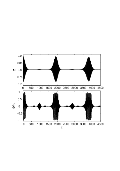
Figure 2: Quantum evolution for $N=350$ BEC atoms and the lattice with $\Lambda=0.2407$. As the initial population we used the Gaussian distribution $C_{k}(0)=\exp\{ik-(k-k_{c})^{2}/(2\sigma^{2})\}$ with $\sigma^{2}=50$ and $k_{c}=50$.

Although collapse of Rabi oscillations was earlier observed in pure mean-field models (see  KKS ; BKK ), the nature of the phenomenon considered here is very different. Suppression of the oscillations in the case of spatially extended systems is related to development of inhomogeneous spatial patterns, mainly related to modulational instability of one of the states. In the case at hand, however the effect is essentially quantum and disappears in the meanfield limit (where $N\to\infty$). This is clearly illustrated in Fig. 3, where we compare the results of the quantum dynamics with its mean-field limit at earlier stages of the evolution.

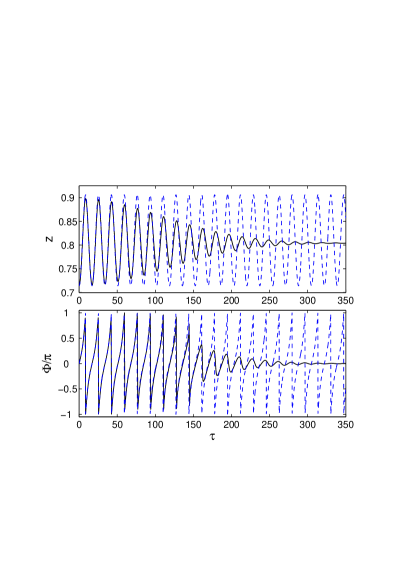
Figure 3: The initial quantum evolution (solid lines) vs meanfield evolution (dashed lines) for parameters as in Fig. 2.

Now we turn to the Case II, where $\Lambda>\Lambda_{c}$, which is shown in Figs. 4 and 5. The main feature of this situation is that as a result of quantum collapse both states become equally populated ($z\to 0$), what is also in accordance with the meanfield dynamics (c.f. Figs. 2 and 4). The revival occurs at latter times $\Delta\tau\sim 3000$.

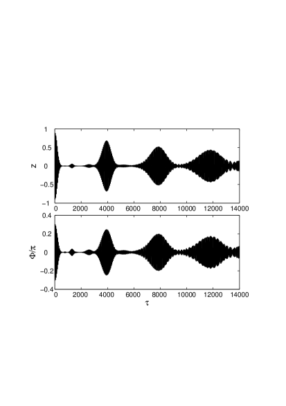
Figure 4: Quantum evolution for $N=500$ BEC atoms and the lattice with $\Lambda=0.404$. The initial condition used is $C_{k}(0)=\exp\{-(k-k_{c})^{2}/(2\sigma^{2})\}$ with $k_{c}=25$ and $\sigma^{2}=50$.

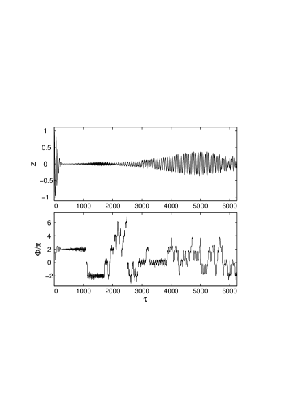
Figure 5: Quantum evolution for $N=1000$ BEC atoms and the lattice with $\Lambda=0.404$. The initial condition used is $C_{k}(0)=\exp\{ik-(k-k_{c})^{2}/(2\sigma^{2})\}$ ($\Phi(0)=2$) with $k_{c}=10$ and $\sigma^{2}=50$.

In all the figures one can observe that the period of the Rabi oscillations is very accurately reproduced by the mean-filed approximation, i.e. by the formulas (28), (29), (30), and (30). In particular, Figs. 3 (or  2) and  5 correspond to the Cases 1 ( with $z=0.72$ and $E\approx-0.033$) and 3 (with $z=0.98$ and $E\approx-0.0059$) described in Sec. III.2. Then using (28) and (31) one computes $T\approx 16.86$ and $T\approx 51.99$, what matches very well with the periods obtained from the direct numerical simulations. The described behavior has simple physical explanation: passage to the mean-field description is performed at a constant $gN$, i.e. at a constant effective nonlinearity of the system. Meantime, the tunneling time depends on the relative value of the nonlinear interaction term, i.e. on $\Lambda$.

Comparing Figs. 2 and 4 one observes the expected effect of the delay of the quantum collapse in terms of the dimensionless time $\tau$ with increase of the number of particles. At the same time the numerical simulations did not reveal any significant effect of the initial phase mismatch $\Phi(0)$ on the collective dynamics.

Another relevant parameter is the initial distribution of the atoms. Clearly, the closer is the initial distribution of atoms (defined by $k_{c}$ and $\sigma$ in the numerics) to the one violating the mean-filed assumptions, when almost all of the atoms are at one of the X_j points, the further is the dynamics from the quasi-classical one, which is reflected in Fig. 5 in the fact that the collapse time of the oscillations is twice as smaller as that of Fig. 4 for twice as much number of atoms. Also, in Fig. 5 the phase dynamics at the recurrence of quasi-classical relative population oscillations contains the quasi-classical oscillations interrupted by the $2\pi m$ jumps.

V Discussion and conclusion

In the present paper we have considered the quantum tunneling of a Bose-Einstein condensate loaded in a two dimensional lattice. The considered tunneling occurs between two stable states, hence allows us to restrict the consideration to a spatially homogeneous model. Such a model, in the rotating wave approximation, was further reduced to the effective two-state system, where both states possess the same energies. The considered tunneling is essentially nonlinear and related to the four wave-mixing due to the two-body interactions (in a pure linear system such a tunneling cannot occur because of violation of the momentum conservation).

The main finding of the work is the quantum collapse and revivals of the Rabi oscillations between the tunneling states, which are suppressed in the mean-field approximation due to the fact that tunneling between two equal-energy states result in configurations of low atomic population of one of the states and thus, strictly speaking, cannot be described in terms of the mean-field approximation. Nevertheless, the latter approach turns out to be useful in predicting different regimes of the tunneling, with collapse occurring to either equal or disbalanced populations of the states, and for accurate estimate of the frequency of the Rabi oscillations (i.e. the tunneling time).

Existence of a well-defined frequency of the oscillations and the difference in spatial patterns of the condensate in different X-states of the lattice suggest a way of experimental observation of the phenomenon, which could be based, for example, on direct imaging at specific moments of time. To estimate the physical time scale corresponding to the period of the Rabi oscillations, we consider a condensate of ⁸⁷Rb atoms, with the $s$-wave scattering length $a_{s}=5.25nm$, which is tightly trapped, say in $y$ direction, with the respective linear oscillator length $\ell=0.1\,\mu$m, and has $N=350$ atoms occupying $M=25$ sites of a lattice with the period $d=2\,\mu$m (i.e. the 2D optical lattice is imposed in the $(x,z)$ plane and has 5 cells in each direction). In this case $g$ (the 2D nonlinear constant) is given by $g=2\sqrt{2\pi}\hbar^{2}a_{s}/m\ell_{y}$. Then using the data from Fig. 2 (also Fig. 3) we obtain that the dimensionless period $T\approx 16.68$ in the physical units is $T_{Rb}\approx 0.00655\,$s. Thus, taking into account that the collapse and subsequent revival would occur after about $1\,$s and $10\,$s, respectively, we see that this is a relatively slow process. This is an expected slowness as far as in this example we used a small number of atoms not providing effective enough tunneling due to the two-body interactions. The collapse and revival time could be reduced by using a larger condensate, however, for a very large number the collapses and revivals will be suppressed because of approaching the mean-field limit. An alternative way to accelerate the quantum collapse, and thus make easier its observation is to use more light atoms, say sodium ones, or by increasing the scattering length.

A number of important questions, however, are left for further studies. Among them we mention the resonant interaction of more than two states, the quantum theory of nonlinear Landau-Zener tunneling, the study of interplay of quantum collapse and of modulational (dynamical) instability in the case when the spatial extension of the system is taken into account and the states among which the tunneling occurs possess different stability properties (what is an intrinsic feature of the nonlinear systems), the effect of opening or closer of the total gap in the lattice, the interplay between the quantum collapse and the dynamical collapse (also called the blow up) which can occur in Bose-Einstein condensates with attractive atomic interactions, etc.

- (1) C. W. Gardiner, Phys. Rev. A 56, 1414 (1997)
- (2) B. Wu and Q. Niu, Phys. Rev. A 61, 023402 (2000); New J. Phys. 5, 104 (2003); O. Zobay and B. M. Garraway, Phys. Rev. A 61, 033603 (2000).
- (3) V. V. Konotop, P.G. Kevrekidis, and M. Salerno, Phys. Rev. A 72, 023611 (2005).
- (4) V. S. Shchesnovich and S. B. Cavalcanti, J. Phys. B: At. Mol. Opt. Phys. 39, 1997 (2006).
- (5) O. Morsch, J. H. Müller, M. Cristiani,D. Ciampini, and E. Arimondo , Phys. Rev. Lett. 87, 140402 (2001); M. Cristiani, O. Morsch, J. H. Müller, D. Ciampini, and E. Arimondo Phys. Rev. A 65, 063612 (2002); M. Jona-Lasinio, O. Morsch, M. Cristiani, N. Malossi, J. H. Müller, E. Courtade, M. Anderlini, and E. Arimondo, Phys. Rev. Lett. 91, 230406 (2003); ibidem 93, 119903 (2004).
- (6) B. Wu and Q. Niu, Phys. Rev. A 64, 061603 (2001); V. V. Konotop and M. Salerno, Phys. Rev. A 65, 021602 (2002); M. Machholm, C. J. Pethick, and M. Smith, Phys. Rev. A 67, 053613 (2003); Yi. Zheng, M. Kostrun, and J. Javanainen, Phys. Rev. Lett. 93, 230401 (2004).
- (7) F. Cataliotti, L. Fallani, F. Ferlaino, C. Fort, P. Maddaloni, and M. Inguscio, Wew J. Phys. 5, 71 (2003); L. Fallani, L. De Sarlo, J. E. Lye, M. Modugno, R. Saers, C. Fort, and M. Inguscio Phys. Rev. Lett. 93, 140406 (2004).
- (8) V. A. Brazhnyi, V. V. Konotop, and V. Kuzmiak, Phys. Rev. Lett. 73 150402 (2006)
- (9) M. Jääskeläinen and P. Meystre, Phys. Rev. A 71, 043603 (2005)
- (10) M. Jääskeläinen, W. Zhang, and P. Meystre, Phys. Rev. A 70, 063614 (2004)
- (11) V. M. Kenkre and D. K. Campbell, Phys. Rev. B 34, 4959 (1986); S. Raghavan, A. Smerzi, S. Fantoni, and S. R. Shenoy, Phys. Rev. A 59, 620 (1999).
- (12) V. A. Brazhnyi, V. V. Konotop, V. Kuzmiak, and V. S. Shchesnovich (submitted)
- (13) J. I. Cirac, R. Blatt, A. S. Parkins, and P. Zoller, Phys. Rev. A 49, 1202 (1994)
- (14) P. A. Braun, Rev. Mod. Phys. 65, 115 (1993).
- (15) A. Vardi and J. R. Anglin, Phys. Rev. Lett. 86, 568 (2001); J. R. Anglin and A. Vardi, Phys. Rev. A 64, 013605 (2001).
- (16) J. M. Ziman The principles of the Theory of Solids (Cambridge: Cambridge University Press, 1972)
- (17) M. Greiner, et al., Phys. Rev. Lett. 87, 160405 (2001); Nature 419, 51 (2002).
- (18) Eqs. (21a), (21b) can also be derived from the Hamiltonian (5) of Ref. BKK .
- (19) W. V. Houston, Phys. Rev. 57, 184 (1940).