Bicocca-FT-08-02
NSF-KITP-07-212
Eikonal Methods in AdS/CFT:
BFKL Pomeron at Weak Coupling
Abstract
We consider correlators of super Yang Mills of the form , where the operators and are scalar primaries. In particular, we analyze this correlator in the planar limit and in a Lorentzian regime corresponding to high energy interactions in AdS. The planar amplitude is dominated by a Regge pole whose nature varies as a function of the ’t Hooft coupling . At large , the pole corresponds to graviton exchange in AdS, whereas at weak , the pole is that of the hard perturbative BFKL pomeron. We concentrate on the weak coupling regime and analyze pomeron exchange directly in position space. The analysis relies heavily on the conformal symmetry of the transverse space and of its holographic dual hyperbolic space , describing with an unified language, both the weak and strong ’t Hooft coupling regimes. In particular, the form of the impact factors is highly constrained in position space by conformal invariance. Finally, the analysis suggests a possible AdS eikonal resummation of multi-pomeron exchanges implementing AdS unitarity, which differs from the usual –dimensional eikonal exponentiation. Relations to violations of –dimensional unitarity at high energy and to the onset of nonlinear effects and gluon saturation become immediate questions for future research.
1 Introduction
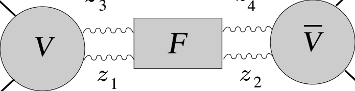
String interactions in flat space are dominated, at tree level and in the eikonal regime , by a leading Regge pole associated to the exchange of string excitations of increasing spin, starting with the massless graviton. The same behavior is expected for high energy interactions of strings in AdS [1, 2, 3, 4, 5, 6, 7]. In this case, the flat space –matrix is substituted by correlators in the dual conformal field theory, and the analogous of a to scattering amplitude is given by CFT correlators of the form
| (1) |
CFT positions play the role of momenta in AdS, with the analogous of a scattering process achieved by choosing Lorentzian kinematics with in the future of , in the future of , and with the pairs , and , spacelike related [2, 3, 4], as shown in figure 1. The relevant AdS eikonal regime is then obtained by sending . Contrary to a Euclidean configuration, the amplitude is not dominated in this limit by the OPE, but by the exchange of operators of maximal spin [3], as in flat space. Moreover, whenever the spin of the exchanged operators is unbounded, one must use Regge techniques, as discussed in detail in [7, 6].
We shall focus our attention on the canonical example of Type IIB strings on AdSS5, dual to super Yang–Mills (SYM) [8]. The planar contribution to the full amplitude corresponds to tree level string interactions in AdS and will be dominated by a Regge pole whose trajectory will depend on the ’t Hooft coupling of the Yang–Mills theory, or dually on the AdS radius in units of string length . Moreover, the trajectory depends, as in flat space, on the transverse momentum transfer . At large coupling , strings move almost in flat space, and the Regge spin is given essentially by the flat space trajectory so that [1, 7]
Only the third term is not determined by the flat space limit, since it vanishes for . It is fixed, however, by the requirement that the graviton is massless in AdS for any value of , which translates to , as shown in [7]. This implies that, as we decrease the radius of AdS, the intercept decreases from the flat space result.
This paper is concerned, on the other hand, with the leading Regge pole of SYM at weak ’t Hooft coupling. The high energy behavior of SYM, when analyzed in momentum space in four dimensions and in the high energy regime , is dominated by the exchange of a single perturbative BFKL pomeron [9, 10, 11]. To leading logarithmic order, the BFKL pomeron is independent of the underlying supersymmetry, and dominates high energy interactions as in conventional QCD. At leading order in , the pomeron is nothing but a pair of gluons in a color singlet state of effective spin . Moreover, the leading corrections in modify this trajectory to
Note that the leading intercept increases for small , justifying the conjecture [1] that the pomeron trajectory is nothing but the leading string trajectory at weak coupling, corresponding to string exchange in a highly curved AdS spacetime.

The usual treatment of BFKL pomeron exchange is conducted in –dimensional momentum space. More precisely, external scattering states are chosen to be momentum eigenstates with appropriate kinematics, whereas the internal pomeron propagator is best described in position space on the space transverse to the interaction [10]. However, as discussed above, the more appropriate way to analyze SYM correlators, in view of the AdS/CFT duality, is to consider them as “–matrix elements” of interactions in AdS, with CFT positions playing the role of AdS momenta. It is then natural to reconsider the BFKL analysis with external states labeled by positions, in the kinematical limit described at the beginning of this introduction. We shall address this issue, sharpening the conjectured duality between pomeron exchange and string exchange in AdS. More precisely, we analyze the couplings of external states to the BFKL pomeron – the so–called impact factors – in position space, heavily using the conformal invariance of the transverse conformal space and of its holographic dual hyperbolic –space . The formalism allows us to describe, in a unified and coherent fashion, the Regge pole exchange at weak coupling as well as at strong coupling.
We shall work mostly with a specific simple example, where the operators and are given by the chiral primaries and , with and two of the complex adjoint scalar fields of SYM. The correlator (1) is known both at weak coupling [12] at order , as well as at strong coupling using the AdS/CFT duality [13], and it is therefore a good example to describe the general theory. In section 2, after reviewing some facts on Regge theory in CFT’s [7], we summarize the general results of the paper. Sections 3 and 4 are then devoted to the proof of these results. More precisely, in section 3 we discuss the general BFKL formalism in position space for generic scalar operators and , whereas in section 4 we specialize to the operators and , deriving their impact factors in position space. Since section 2 contains a summary of our main findings, as well as open questions, we found it redundant to include a concluding section.
The present paper is focused mostly on the analysis of the planar limit of the correlator (1), which corresponds to the exchange of a single pomeron. On the other hand, due to the raising intercept , a single pomeron exchange generates a total cross section that grows with energy and inevitably violates unitarity bounds in four dimensions [14, 15, 16]. At weak coupling, it is well known that this problem cannot be cured uniquely by eikonalizing the pomeron exchange, but one must also consider non–linear pomeron interactions which tame the high energy growth and restore unitarity. In the context of hadronic interactions, this corresponds to the saturation of the hadron gluon transverse density at small values of Bjorken and is quite relevant to experimentally accessible regimes in deep inelastic scattering experiments [14, 15, 17]. Our position space formalism, on the other hand, is related from the start to interactions in AdS and, in fact, admits an eikonalization with respect to geodesic motion in five dimensions [4, 7]. Moreover, the AdS eikonal is clearly valid at strong ’t Hooft coupling, where, for a large range of AdS impact parameters, the phase shift is of order one and needs to be eikonalized even though one is quite far from the critical impact parameter where non–linear gravitational effects start to become important and drive black hole formation. It is then tempting to speculate that, even at weak coupling, the –dimensional AdS eikonal resummation is valid in some range of the kinematical parameters, and is relevant for the physics of high energy scattering before the onset of gluon saturation. These issues, as well as the fascinating relation between gluon saturation and black hole formation where non linear effects become important [18, 19, 20], could lead to a possible experimental observation of the gauge/gravity correspondence and will be the subject of our future investigations [21].
2 General Results
2.1 Review of Regge theory for CFT’s
We consider a –dimensional conformal field theory defined on Minkowski space . We parameterize points with two light–cone coordinates and with a point in the Euclidean transverse space , and we choose the metric . We will be interested in the analysis of the correlator
| (2) |
where and are scalar primary operators of dimension and , respectively. By conformal invariance, the above correlator can be expressed as
where the reduced amplitude depends on the cross–ratios defined by [22]
The reduced amplitude is originally defined for Euclidean configurations with and , where it coincides with the amplitude of the Euclidean continuation of the CFT at hand. On the other hand, here we are interested in intrinsically Lorentzian configurations, with
| (3) | |||
The best intuition for the above configuration comes from thinking of the CFT positions as points on the boundary of global AdS, as in figure 1 in the introduction. The conditions (3) then corresponds to a true Lorentzian scattering process in the dual AdS geometry. We shall also require that
| (4) |
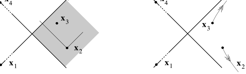
This condition is not essential, but streamlines considerably our discussion [7]. For such configurations, shown in figure 2a, the relevant reduced amplitude is given by a specific analytic continuation of , as described in figure 2b and in detail in [4, 7]. We shall be interested in the study of the amplitude in the limit , which implies .

To clarify the underlying geometry of the Lorentzian amplitude, it is best to introduce the concept of transverse conformal group [7]. Consider the correlator (2) as a function of two points, and , fixing the positions of and . The subgroup of the conformal group which leaves the points and fixed is given by . This fact is manifest if we use conformal symmetry to send the point to the origin and the point to infinity, which can be achieved, for instance, by first translating and then by performing a special conformal transformation , with and . Under these transformations the points and are mapped, respectively, to and , with
The vectors and are defined up to the residual conformal symmetry. This is given by rotations, under which and transform as vectors, and by dilatations, under which and . Moreover, for the kinematics (3) and (4), is in the future of and
where is the future Milne wedge. The reduced amplitude can then be written as
and depends only on the conformally invariant cross-ratios
We are interested in the limit of the reduced amplitude. As shown in [3], this limit is not dominated by the OPE and therefore by operators of lowest conformal dimension, as in the Euclidean version of the theory, but by the exchanged operators of maximal spin. Whenever the exchanged spin is unbounded, the limiting behavior must be analyzed using Regge techniques [7]. In the presence of a Regge pole with trajectory , the limit of the reduced amplitude reads111For simplicity of notation, here and in the rest of the paper we write instead of the more cumbersome expression .
where is the pole residue and where , given explicitly in [7] and in section 3.4 of this paper, computes radial Fourier transforms in the transverse hyperbolic space and solves the homogeneous equation . In CFT’s with an AdS5 string dual, the hyperbolic space plays the role of the space transverse to the interaction and measures transverse momentum transfer, with the AdS radius. Therefore, for large , we may think of as momentum transfer in AdS5.
2.2 super Yang Mills
We shall focus our attention on the canonical example of , SYM with ’t Hooft coupling . The theory is dual to IIB strings on AdSS5, with AdS radius and –dimensional Newton constant . In particular, as a basic example, let us consider the correlator (2), with
where and are two of the three complex scalar fields of the theory and is a normalization constant fixed so that the –point functions and are canonically normalized to . The operators are chiral primaries and are not renormalized, with . Therefore, the reduced amplitude will read
where represents the disconnected part , whereas represents the planar contribution to the amplitude, dual to tree–level string interactions. The planar contribution depends non–trivially on the ’t Hooft coupling and should be dominated, in the Lorentzian regime described above, by the Regge pole associated to the exchange of the tower of massive string states of lowest twist. In particular, we expect that the planar contribution should be given by
| (5) |
where we have explicitly shown the dependence of the trajectory and of the residue function .
2.3 Large ’t Hooft coupling
At large ’t Hooft coupling, the dominant Regge trajectory is dual to graviton exchange in AdS. As shown in [1, 7], the trajectory has a large expansion given by
Moreover, in the limit , the residue function is given by [7]
The term represents the graviton propagator, dual to the CFT stress–energy tensor of dimension , which corresponds222As discussed in [7], we normalize so that CFT dimensions are given by . to . The function is given explicitly by
and represents the minimal coupling of the dimension external scalars to the exchanged trajectory of spin . In the limit , one has that corresponding to the usual gravitational field, so that
2.4 Weak ’t Hooft coupling
The main focus of this paper is devoted, though, to the analysis of at weak coupling . The planar amplitude has been computed to order in [12], with explicit result
| (6) | |||
where
Using the fact that for the analytic continuation of is given by , it is easy to show that, in this limit, the Lorentzian amplitude is dominated by the term proportional to , and it is explicitly given by
| (7) |
The above expression is invariant under rescalings , and it therefore corresponds to the contribution of a leading Regge pole of spin . Moreover, explicitly computing the radial Fourier transform in the transverse space , one may show that (7) corresponds to333Defining , one has that . Since is given by (5) for , one has that , as shown in [7].
| (8) |
where
| (9) |
As we shall review in more detail in section 3, the above result is dominated by the Regge pole of the perturbative hard BFKL Pomeron [9, 10, 11], with trajectory given by the famous expression
which converges to for . In the next section, we shall formulate the usual BFKL formalism completely in position space and explicitly derive (8). The factor corresponds to the pomeron propagator, whereas and correspond to the couplings of external states to the pomeron, usually called impact factors in the literature. We shall derive the explicit leading order expressions (9) directly in perturbation theory in position space in section 4, thus rederiving (8) without the need of the full result (6).
The use of position space techniques streamlines considerably the usual computations based on the momentum space BFKL impact factors. In particular, we shall show how the position space formalism, which uses heavily the invariance under the transverse conformal group , immediately implies that only the part of the BFKL kernel gives non–vanishing overlap with impact factors of scalar external states.
2.5 Eikonalization of the pomeron exchange and saturation
Let us conclude this introductory section with some more speculative considerations. Recall from [7] that the contribution from a single pomeron exchange grows too fast at high energy and eventually violates the unitarity bounds. At large impact parameters, we expect that one should be able to restore unitarity by considering multiple pomeron exchanges using eikonal methods. The CFT extension of the usual eikonal resummation, which corresponds dually to eikonalization in the dual AdS geometry, was developed in [3, 4, 5] and was generalized to Regge pole exchanges in [7, 6]. Let us first recall the basic facts. In the regime of small , the CFT amplitude admits an impact parameter representation in AdS given by [3, 7]
| (10) |
where the Fourier integral is supported only in the future Milne cone . The function plays the role of the phase shift and depends on the invariants and , which correspond to energy–squared and impact parameter in the dual AdS geometry. As in flat space scattering, the impact parameter representation approximates the AdS (conformal) partial wave decomposition for large values of the impact parameter and energy. In analogy with flat space, AdS unitarity should be diagonalized by the partial wave decomposition and should simply corresponds to the requirement . Let us note, though, that the status of unitarity in AdS interactions is not on the same firm theoretical grounds as the corresponding statements in flat space, due to the lack of asymptotic states and of an explicitly unitary –matrix.
When , there is no AdS interaction and . We may then define the planar phase shift by
Whenever the planar amplitude is dominated, for small , by a Regge pole and is given by (5), the above expression can be inverted to get
valid for large , with defined by
Note that we have
| (11) |
In the eikonal approximation, valid in principle for large values of the AdS energy–squared and impact parameter , the full phase shift is approximated by the planar contribution . The eikonal amplitude, resumming multi–pomeron exchanges, may then be written as
| (12) |
The eikonal expression (12) would then automatically implement unitarity both at weak and at strong coupling for . In particular, the limit (11) given by
has negative imaginary part, as expected.
An important unresolved issue concerns the relation of the –dimensional AdS eikonal expression (12) to the standard eikonalization of the correlator (2) in four dimensions. In fact, it is well known that unitarization of the weak coupling BFKL pomeron exchange using –dimensional eikonal techniques fails to reproduce the correct physics at large energies and must be supplemented by the far more complex analysis of non–linear pomeron interactions, which in turn lead to the phenomenon of gluon saturation in the structure functions of the scattering states (see [15] for reviews and for an extensive list of relevant references). On the other hand, multi–pomeron interactions have never been analyzed using the AdS expression (12). It is quite reasonable that, for a certain range of AdS impact parameters, the planar approximation to the phase shift is still valid even when the phase shift is of order one and a single exchange violates the unitarity bound. Let us note that eikonal resummations are possibly the simplest technique to analyze the ambient geometry, since it is inherently based on geodesic motion in the spacetime where interactions take place. Moreover, saturation effects, where non–linear pomeron interactions are relevant, have already been seen at present accelerators. It is then quite conceivable that, for carefully chosen external kinematics, interactions are approximated by expression (12), thus showing experimentally the duality between field theories and gravity. We plan to address some of these issues in [21].
3 BFKL Analysis in Position Space
3.1 The BFKL kernel at vanishing coupling
High energy interactions in gauge theories are dominated by hard pomeron exchange for . In the Born approximation, the leading contribution at high energies comes from the exchange of a pair of gluons in a color singlet state, and amplitudes444In order to have a consistent notation when discussing CFT correlators, we incorporate, in the definition of the amplitude, the factor of , using the convention as opposed to the more standard field theory convention . are conveniently written as [9, 11]
| (13) |
Let us describe qualitatively the main features of (13), using as an aid figure 3. First of all, the overall energy dependence shows that we are exchanging a Regge pole with effective spin . At high energies, the exchanged gluons are essentially transverse, and are replaced by a pair of massless propagators
| (14) |
in transverse space , where the are the gluon transverse positions. The coupling of the pair of gluons to the scattering states is, on the other hand, described by the impact factors and . These factors depend on the transverse momentum transfer in and also on other features of the external incoming and outgoing states, like virtualities and polarizations, which we do not show explicitly. Whenever the scattering states have vanishing color charge, the impact factors satisfy the infrared finiteness condition [11]
| (15) |
and similarly for . Finally, note that the amplitude is mostly real (imaginary in the usual field theory convention), leading to an imaginary phase shift.
Let us first concentrate on the pomeron kernel (14) describing the propagation of the two transverse gluons. At finite ’t Hooft coupling , the leading corrections to (14) are described by the BFKL equation [9, 11]. As noted by Lipatov in [10], the BFKL equation is invariant under transverse conformal transformations of if we assume that transforms like a –point function of scalar primaries of vanishing dimension. It is then natural to look for solutions depending on the transverse harmonic cross–ratios
| (16) |
Clearly, (14) is not invariant under conformal transformations of . However, we are free to add to the BFKL kernel any function which is independent of at least one of the ’s, since physical amplitudes (13) are obtained by integrating against impact factors satisfying (15). Therefore, we may substitute the kernel (14) with the equivalent conformally invariant function
| (17) |
3.2 Explicit transverse conformal invariance
In order to render the transverse conformal invariance manifest, it is best to work in Minkowski space on which the transverse conformal group , introduced in section 2.1, acts naturally. This discussion entirely parallels the case of the conformal group of –dimensional Minkowski spacetime, whose action on the light–cone of an embedding space is linear, as reviewed in [2, 3].
Let us recall some basic notation schematica, denote with the future Milne wedge, with the future light–cone and with the hyperbolic –space of points with , holographically dual to the transverse space of the gauge theory. The boundary of can also be described invariantly by using the embedding space . More precisely555In [2], the analogous statements where discussed for the boundary of the full AdS5, seen as light rays in the embedding space ., we may think of transverse space as light-rays in , i.e. points such that and , identifying points related by a positive rescaling factor , as represented in figure 4. Transverse space is then recovered by taking an arbitrary slice of the light–cone , choosing a specific representative for each ray (for an extensive discussion of this point, see for instance [23]). We shall denote with any given choice of such slice. The standard space is recovered with the usual Poincaré choice , so that a generic point is parameterized by points as
| (18) |
Note that, for two points and of the form above, the inner product
computes the usual Euclidean distance , so that the cross–ratios (16) can be written invariantly as
and the BFKL kernel becomes a function of the invariants , invariant under rescalings .

More generally, consider a generic function invariant under . It will generically depend on the invariants . On the other hand, if we assume that has weight in the –th entry, scaling as
the number of independent invariants is reduced to cross–ratios. Finally, if of the points are boundary points on the light-cone and therefore satisfy , the total number of cross–ratios is reduced to
| (19) |
The BFKL kernel has , and therefore it has independent cross–ratios, as any CFT –point correlator.
We may obtain conformally invariant functions via integration. More precisely, we may consider the integral
over hyperbolic space , which clearly defines a conformal function of the remaining points . More subtle is to construct conformally invariant functions via integration over the boundary , due to the arbitrariness in the choice of slice of . One can easily show that the integral
is independent of the choice of slice, and therefore conformally invariant, whenever , i.e. whenever
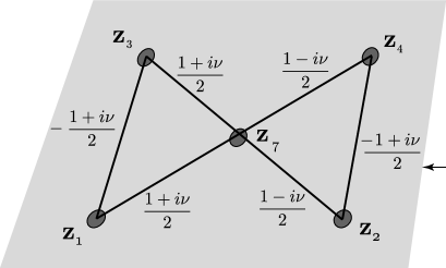
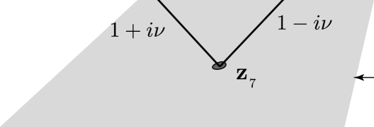
3.3 The component of the BFKL propagator
To analyze the –point kernel (17), it is best to construct more basic conformal building blocks. Consider a conformal function dependent on three boundary points , respectively with weights . There are no cross–ratios and, up to a multiplicative constant, it is given uniquely by the –point coupling of scalar primaries
We may then consider the conformally invariant integral
| (20) |
shown in figure 5, where the total weight of the integrand in is correctly chosen to be . For any value of , the above integral defines a conformal function of the four points points with vanishing weights.
Consider now the leading BFKL propagator (17). In general, it can be written as a superposition of integrals of the form (20) with a more general integrand [10]. The integrand itself is always constructed from the product of –point functions with an intermediate state, at the point , of general spin . However, as we shall demonstrate later, whenever we compute amplitudes (13) with external scalar operators, the contributions from the terms with vanish due to conservation of transverse spin. The relevant part of the BFKL kernel can then be written as a superposition of integrals of the form (20) with varying . More precisely, we may replace (17) with the expression [10]
| (21) |
3.4 The amplitude in position space
In this paper, we are mostly interested in the analysis of the Lorentzian amplitude
| (22) |
in position space, where we recall that and are in the future Milne wedge . In particular, we focus our attention on the limit. As discussed in [7] and reviewed in section 2, the limit of the planar amplitude is dominated by a leading even signature Regge pole, whose spin depends on the ’t Hooft coupling . For large , the pole corresponds to a reggeized spin– graviton exchanged in the bulk of AdS, whereas for small the pole corresponds to the exchange of a hard BFKL perturbative pomeron of spin approximately . Therefore, recalling that the reduced amplitude scales as for a pure spin– pole [7], we deduce that, in the limit , the amplitude will be invariant under rescalings of and so that
| (23) |
The amplitude will then depend uniquely on the geodesic distance between the points and in the transverse hyperbolic space H3, and has the Fourier decomposition (5) given by
| (24) |
As shown in appendix A.3, the Fourier basis of radial functions is conveniently given by the following integral representation666In terms of the geodesic distance in , given by , we have that , as discussed in [7].
| (25) |
as shown graphically in figure 6.
3.5 Impact factors in position space
We are now in position to introduce the BFKL formalism in position space, applying it to the computation of in the limit and to leading order in . The amplitude will be given again by an expression similar to (13), but now the external state impact factors and are not labeled by the exchanged transverse momentum , but by the positions and in the Milne cone . Therefore we expect the amplitude to be given by an integral of the form
| (26) | ||||
Note that we replaced the integrals over the transverse space with integrals over an arbitrary section of the light–cone .
The form of the impact factors and is almost fixed by conformal invariance. In fact, must scale in and with weight , in order for the integrals over to give a conformally invariant result. Moreover, must be invariant under rescalings of in order to satisfy (23). Finally, since , there is a unique scale–invariant conformal cross ratio which can be constructed from , and , given by
| (27) |
The impact factor must then be of the general form
Let us first note that, since and , the cross–ratio satisfies
This can be shown simply by using symmetry to rotate and respectively to and , possibly after an immaterial rescaling. Then, parameterizing , we obtain and
The infrared finiteness condition (15) may also be written simply as
| (28) |
In fact, by conformal invariance and scaling, we know that the integral (15) must be given by
where the constant can be computed as
Similar equations apply to .
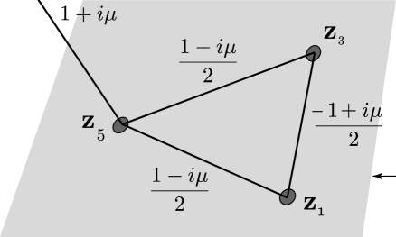
3.6 A basis for impact factors
Now we discuss a convenient basis for the functions satisfying (28). We shall consider the following conformal integral
| (29) |
graphically shown in figure 7, where we defined
By conformal invariance, the integral (29) is only a function of the cross–ratio . As shown in appendix A.5, it is explicitly given by
| (30) |
where
with the hypergeometric function . The functions are a convenient basis for the impact factor , which we write as
| (31) |
where we have chosen
without loss of generality. Moreover, we shall use the same label for the impact factor both as a function of and of the transformed variable , with the hope that the difference will be clear from context.
Consider the infrared condition (28). Since777The integral diverges at for real and it is computed by analytically continuing the result obtained for .
is odd in , it is clear that satisfies automatically (28).
In particular, let us consider given by a pure power . To satisfy the infrared condition (28), the full expression must be of the form
As shown in appendix B, this corresponds to a transform in (31) given by
In particular, we shall see that the relevant impact factor in section 4 will be
corresponding to
| (32) |
3.7 Computation of the BFKL amplitude
We are now in position to compute the amplitude (24) starting from impact factors and . More precisely, we shall show that the new BFKL integral representation (26) gives an amplitude of the form (24) with
| (33) |
This will be the main result of this section, showing (8).
We start by replacing, in the amplitude (26), the part of the BFKL kernel (21), thus obtaining
| (34) | ||||
We shall first focus on the second line of this expression. Replacing the integral representation (31) for the impact factor , we obtain the following conformal integral
| (35) |
shown graphically in figure 8.
Let us note that the second line of this expression, highlighted in figure 8 with a continuous line, is almost completely fixed by conformal invariance. It is, in fact, a conformal function with weights and , respectively in the two entries. Since the only conformal invariant is , the function must vanish for and must be proportional to for . The second possibility is a contact –function contribution , defined as usual by
| (36) |
The function is conformally invariant whenever the weights in and sum to . In fact, if is of weight , the above integral is well defined when the weight in is and, for (36) to be satisfied, the weight in must be . Therefore, the –function contribution to can be non–vanishing only for . The exact integral has been explicitly computed by Lipatov in [10], with the result
We may then complete the computation of (35), performing the integral in to obtain
where in the second term we have used the conformal integral
from appendix A.2. Finally, computing the integral and using the fact that we obtain the final result for the second line of (34)
We may carry out an equivalent computation for the second impact factor . Combining the two expressions, we conclude that the BFKL amplitude (34), graphically shown in figure 9,
3.8 Vanishing of the contributions
We have previously claimed, without proof, that the unique contribution to the BFKL amplitude (26) comes from the part (21) of the complete two–gluon kernel (17), whenever the external states are scalar operators. This fact is now almost trivial to show. In fact, the terms would involve, similarly to the discussion in section 3.7, an overlap integral of the general form (35). The only difference would come from the second line of (35), which would have a –point coupling at points with a spin state located at . The full integral on the second line of (35) would then vanish by conservation of transverse spin, as shown also in [10], since it would connect a spin state at to a spin at .
In this paper we consider only scalar external operators for simplicity. We could have considered more general external states in various representations of the –dimensional conformal group. For example, we could have chosen spin external states. In this case, the impact factors would have a non trivial index structure coming from the external operator at points , and the basis functions (29) need to be modified to include this extra structure. It is natural to expect that this will involve contributions of transverse conformal spin coming from the indices at the two points . This fact was shown in a non–transparent way in [24] for the case , which is relevant to interactions with off–shell photons in deep inelastic scattering processes at small values of Bjorken .
4 Impact Factors in SYM
In this section, we apply the position space BFKL formalism to the computation of the SYM –point function
discussed in section 2. Recall that the operators and are given by
with and adjoint complex scalar fields, and are normalized so that their –point function is
In the conventions of appendix C, the constant is given by
In particular, we shall compute explicitly the impact factors and for the operators and to leading order in perturbation theory, thus showing (9).
4.1 Some kinematics
To simplify the computation, it is convenient to carefully choose the kinematics. We shall write to compactly show the light–cone and transverse components of a vector . Following [7], we choose
and we shall consider the limit . The conditions (3) and (4) then imply that
and that is in the future of . In the limit the expressions for in section 2.1 simplify to
Recall that are defined up to the residual transverse conformal symmetry. Therefore, rescaling and , and boosting , we obtain the expressions
as in [7]. We can further simplify our computations by choosing the transverse parts of the points to vanish, so that
In this convenient kinematical setup, shown in figure 10a, the cross–ratios read
The limit with fixed ratio can then be achieved by sending , with fixed, and , with fixed, as shown in figure 10b.
4.2 Impact factor
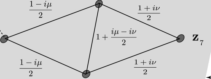
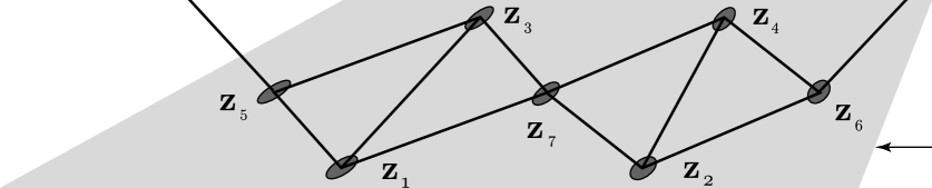
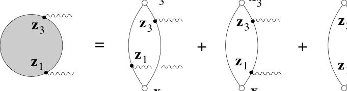
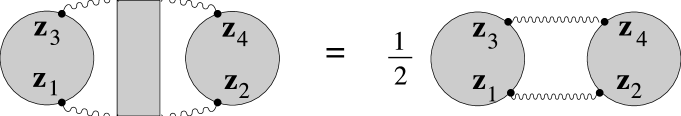
Let us now compute the impact factor for the external operator . A similar computation would give the impact factor of . The leading order diagrams that contribute to the BFKL vertex are given in figure 11, representing the emission of two gluons. The full correlator is then obtained by connecting both vertices and with a pomeron propagator, as described in figure 12, where the factor of is the overall symmetry factor of the diagram. To leading order in perturbation theory, the pomeron propagator is simply given by the exchange of two gluons in a color singlet state.
First we consider the contribution coming from diagram 11a. Since we are interested in the reduced amplitude, we must divide the diagram by the two point function . Fixing for now the position of the gluons at and , the Feynman rules give
where and are the spacetime and color indices of the gluons emitted at . We remark that for now and are points in the physical –dimensional Minkowski spacetime. Later on in the computation these points will collapse to transverse space , and we shall used the embedding formalism described in section 3.2. Simplifying the overall constant in the above expression, we obtain
| (37) |
which represents the emission at and of two gluons in a color singlet, respectively with polarizations and .
As claimed in the previous section, the perturbative computation simplifies considerably if we choose the external kinematics using conformal invariance to set and . Then, the term in brackets in the first line of (37) becomes
A similar expression can be obtained for the other bracket with replaced by . Since the BFKL kinematical limit corresponds to large with the product held fixed, this last expression is dominated by the derivative with , with the leading result
| (38) |
As expected, the emitted gluons have polarization . The computation of the impact factor for the external operator on the other side of the graph is analogous to that of , representing the emission of gluons at and . In this case we set and , and then take the BFKL kinematical limit of large negative with fixed. The emitted gluons will have polarization .
To identify the impact factors and the BFKL kernel one needs to integrate over the internal vertices , , and , and to add the gluon propagators, as described by figure 12. Considering, for example, the vertex at , we shall split the integration in transverse and light–cone directions according to
In the BFKL kinematical limit, the external scalar lines are almost on-shell, while the exchanged gluons are off-shell. When computing the full diagram and integrating over , the residues at the poles in expression (38) are dominant with respect to the residues at the poles in the gluon propagators, as we take large with fixed product . Putting together equations (37) and (38) and dropping the color factor , we conclude that the contribution of the diagram in figure 11a to the impact factor is given by
corresponding to the emission of two gluons in a color singlet, located at and in transverse space and with polarization . These integrals are easily computed by deforming the contour of integration, with the result
| (39) |
Note that, after integrating in and , and taking the BFKL limit , the resulting expression is independent of the other light–cone variables and . The expression depends only on the gluon positions in transverse space . Recalling from section 3.2 that explicit transverse conformal invariance is rendered manifest by considering the usual transverse space as the canonical Poincaré slice of the light–cone , we set . Note that we use the same label both for the original position of the gluons and for the points of the Poincaré slice. This slight abuse of notation is justified by the fact that the relevant transverse parts coincide. It is then immediate to show that the crossratio in (27) is given by
| (40) |
so that expression (39) can be finally written as
| (41) |
where we recall that .
Before we compute the contribution to the impact factor of the remaining diagrams in figure 11, let us consider the BFKL kernel. In the above computation we saw that the residues of the poles at and at are independent of the other light-cone integration variables , , and . Therefore, when computing the full diagram, we can move these integrals to the gluon propagators. It is then clear that the leading order BFKL propagator, as represented in figure 12, is given by
| (42) |
where the spacetime gluon propagators are computed at the above poles and . The overall factor of comes from the symmetry factor of the diagram, while the factors of inside the integration come from the measure. A simple computation, using
gives the transverse gluon propagators888The result is independent of the gauge choice, since the gluon propagators have zero longitudinal momenta and have polarization.
The full amplitude has now the BFKL structure (26). The minus sign of (26) corresponds to the sign of the previous equation. Moreover, to match the convention (14) for the two–gluon leading propagator, we shall multiply, at the end of the computation, the graphs in figure 11 used to compute the impact factor by
| (43) |
where the extra factor of comes from our convention on planar amplitudes (22) which explicitly shows an overall factor of .
Now we compute the contribution to the impact factor of the diagram in figure 11b
which in the BFKL kinematical limit simplifies to
If we write, in the full diagram, the gluon propagators in the Landau gauge, after integrating by parts we may act with the derivatives only on the internal scalar line, with the result
| (44) | |||
The impact factor is then computed after integrating this expression in and . The corresponding residues dominate the residues at the poles of the gluon propagators. First we note that there are singularities in the previous equation for
where the upper and lower signs correspond, respectively, to and . It is then clear that the and integrals are non-vanishing only for , which has the physical interpretation of ordering the interaction vertices in light-cone time. Therefore, we may deform the and integrals in the upper and lower half plane, respectively, picking the contributions of the poles at and at . To compute the relevant residues, let us first note that, in the BFKL kinematical regime, the pole in satisfies and one needs to keep only the dominant term in this limit. A simple computation shows that again gluons with polarizations and give the dominant term. In particular, at the poles we have
where the last limit is obtained for using a standard representation of the –function999For given by and , there are terms in which are also of order . Such terms are proportional to and therefore vanish.. We may now return to the computation of the impact factor in (44), integrating over and we obtain (dropping again the color factor already included in the two–gluon kernel (42))
| (45) |
Again this result does not depend of and so that, when computing the full diagram, their integration can be moved to the gluon propagators in (42). Here one needs to be careful because the contribution of this diagram gives the restriction to the gluon integration. However, repeating the same arguments for the diagram in figure 11c, we recover the whole integration domain. The contribution to the impact factor of the diagrams in figure 11b and 11c is then given by (45).
Defining the delta function along a radial coordinate in as
and using the explicit expression for in (40), we have that
so that (45) reads
| (46) |
Finally, we add the contributions (41) and (46) from all diagrams in figure 11 and multiply by (43) to obtain the correctly normalized impact factor. Taking the large limit we obtain
where we recall that is the ’t Hooft coupling. Note that the above expression satisfies the infrared finiteness condition (28). Using (32), this corresponds to
thus confirming equation (9).
Let us conclude by quoting a simple extension of the result above which we prove in appendix D. We could have considered the more general operator
where again is chosen so that the –point function is normalized to . One may compute the corresponding leading order impact factor quite easily. In fact, the spacetime part of the computation is independent of and the unique difference is related to the color factors. A careful analysis shows that the impact factor in this case is given by
| (47) |
Acknowledgments
LC is funded by the Museo Storico della Fisica e Centro Studi e Ricerche ”Enrico Fermi”. LC is partially funded by INFN, by the MIUR–PRIN contract 2005–024045–002, by the EU contracts MRTN–CT–2004–005104. JP is funded by the FCT fellowship SFRH/BPD/34052/2006. JP and MC are partially funded by the FCT–CERN grant POCI/FP/63904/2005. Centro de Física do Porto is partially funded by FCT through the POCI program. This research was supported in part by the National Science Foundation under Grant No. NSF PHY05-51164.
Appendix A Conformal Integrals
A.1 General integrals
We shall work with vectors in –dimensional Minkowski space with norm , and we define, as in the main text, the usual subspaces
Let us consider first the following conformal integrals101010The normalization chosen for the –functions differs by a factor from the one chosen in [2].
where the points are generically in , or on the boundary , and carry weight , and where we have defined
The above integral converges for
| (48) |
and admits the following Feynman parameter representation [2]
| (49) |
with . We will be more interested in the closely related conformal integral
| (50) |
where we demand that
in order for the result to be conformally invariant. Whenever a point is on the boundary , the convergence of the integral (50) is again ensured by (48), which can also be written as . To compute the integral (50), we choose the Poincaré slice for , given by , so that
Using the usual Schwinger representation for the propagators we obtain
where we defined . Since , the integral over in is gaussian and may be evaluated, with the result
Finally, changing variables , with , we obtain exactly the same expression (49) for the functions , with the restriction . From now on we shall therefore drop the tilde.
Let us conclude by recalling that, if we take of the points to live on future light–cone , the function depends in general on
independent cross–ratios.
A.2 Two point function ,
This is the simplest case, with no cross-ratios. Assuming that and we have that
where the overall normalization is computed from the integral
A.3 Two point function ,
In this case we have one independent cross–ratio, which we choose to be given by
We then have that
where
| (51) |
Using the fact that
we may expand the exponential in (51) in powers of and resum to obtain
Note that, if we choose
the expression for is equal to [7]
where are the radial Fourier functions in . Therefore we have that
A.4 Three point function ,
As is well known, there are no cross–ratios in this case and conformal invariance determines
up to an overall constant , determined by the integral
The integral is easily evaluated with the change of variables
| (52) |
The volume form becomes , and the integral evaluates to [8]
| (53) |
Note that the integral determining converges for , which implies .
A.5 Three point function ,
Let us now assume that is in the bulk of the Milne wedge. We have a single cross–ratio
and the full –function takes the form
with determined by the integral representation
Applying the change of variables (52) we obtain
If we expand the exponential in powers of , and formally use the integral , analytically continued to arbitrary values of , we obtain the formal result
| (54) |
with the constant given in (53). The computation is, on the other hand, only partially correct due to the fact that the integral in is evaluated in the region . To deduce the correct answer, we shall first consider the behavior of the integral for . This is achieved by considering the following configuration , , which has exactly . Choosing the parameterization of given by with , the integral (49) is proportional to
We shall assume, as always, that , and , which implies . The –integral is therefore convergent and can be explicitly evaluated. The above expression becomes
Convergence is now clear. At the integrand behaves as , whereas close to the two leading behaviors are given by and . It is then clear that the correct choice replacing (54) is given by
| (55) |
where the normalization
has been fixed by requiring that whenever the condition holds. In the main text, we are especially interested in the case with . Then we have that
Using the properties of the hypergeometric function, it is now trivial to show that (55) is given by
thus showing (30).
Appendix B Polynomial Impact Factors
Let us consider the integral
with
For , we may close the contour in the region . The contribution to the integral comes from the poles at , with a non–negative integer, so that we obtain the following sum of residues
It can be easily checked that the successive powers for cancel in the above expression, leaving only the initial contribution . We have then obtained that
as we needed to show.
Appendix C SYM Conventions
In this paper, we use standard conventions for SYM. For the convenience of the reader, we quote the most relevant ones. The bosonic part of the SYM action is
with and . The six adjoint real scalars and the gauge field are written, in the basis of generators of , as and , where we choose the normalization
The structure functions are defined as usual as
Two useful relations are
which imply, for instance, that
| (56) |
We define the complex fields by
with propagator
The gauge field propagator in Feynman gauge is also given by the same expression, with the addition of the spacetime metric .
Appendix D Impact Factor for

In this appendix, we shall compute the impact factor for the operator
where the constant is fixed by requiring that the –point function be normalized to . The relevant graphs, to leading order in the ’t Hooft coupling , are shown in figure 13. It is quite clear that the spacetime part of the graphs is identical to that of graphs in figure 11 of section 4.2 for the case . The only difference comes from the color structure. To analyze the color factors, we first write the operator as
where
The coefficient is then clearly given by
Now consider the graphs in figure 13, starting from the simplest graphs 13b,c. In general, the color part is given by
The above expression is proportional to and we may therefore trace over the indices to obtain the normalization constant
Therefore, the relative contribution of the graphs 13b,c, compared to the basic case , is given by
Next we analyze the more complex case of graph 13a. The color part is given by
Again, we trace over to obtain the normalization constant
To compute explicitly the expression above we must compute the expression , given by
Substituting and performing the sum over we obtain
where we used equation (56). We then have that and that
thus proving (47).
References
-
[1]
R. C. Brower, J. Polchinski, M. J. Strassler and C. I. Tan,
The Pomeron and Gauge/String Duality, [arXiv:hep-th/0603115].
J. Polchinski and M. J. Strassler, Hard Scattering and Gauge/String Duality, Phys. Rev. Lett. 88 (2002) 031601, [arXiv:hep-th/0109174]. - [2] L. Cornalba, M. S. Costa, J. Penedones and R. Schiappa, Eikonal approximation in AdS/CFT: From shock waves to four-point functions, JHEP 08 (2007) 019, [arXiv:hep-th/0611122].
- [3] L. Cornalba, M. S. Costa, J. Penedones and R. Schiappa, Eikonal Approximation in AdS/CFT: Conformal Partial–Waves and Finite N Four–Point Functions, Nucl. Phys. B 767, 327 (2007) [arXiv:hep-th/0611123].
- [4] L. Cornalba, M. S. Costa, J. Penedones, Eikonal Approximation in AdS/CFT: Resumming the Gravitational Loop Expansion, JHEP 09 (2007) 037, [arXiv:0707.0120 [hep-th]].
- [5] R. C. Brower, M. J. Strassler and C. I. Tan, On the Eikonal Approximation in AdS Space, arXiv:0707.2408 [hep-th].
- [6] R. C. Brower, M. J. Strassler and C. I. Tan, On The Pomeron at Large ’t Hooft Coupling, arXiv:0710.4378 [hep-th].
- [7] L. Cornalba, Eikonal Methods in AdS/CFT: Regge Theory and Multi-Reggeon Exchange, arXiv:0710.5480 [hep-th].
-
[8]
J. M. Maldacena, The large N limit of superconformal field theories and supergravity,
Adv. Theor. Math. Phys. 2 (1998) 231, [arXiv:hep-th/9711200].
O. Aharony, S. S. Gubser, J. M. Maldacena, H. Ooguri and Y. Oz, Large N Field Theories, String Theory and Gravity, Phys. Rept. 323 (2000) 183, [arXiv:hep-th/9905111]. -
[9]
V. S. Fadin, E. A. Kuraev and L. N. Lipatov, On The
Pomeranchuk Singularity In Asymptotically Free Theories, Phys. Lett.
B60 (1975) 50–52
E. A. Kuraev, L. N. Lipatov and V. S. Fadin, The Pomeranchuk Singularity in Nonabelian Gauge Theories, Sov. Phys. JETP 45 (1977) 199–204
Ya. Ya. Balitsky and L. N. Lipatov, The Pomeranchuk Singularity in Quantum Chromodynamics, Sov. J. Nucl. Phys. 28 (1978) 822–829 - [10] L. N. Lipatov, The Bare Pomeron In Quantum Chromodynamics, Sov. Phys. JETP 63, 904 (1986) [Zh. Eksp. Teor. Fiz. 90, 1536 (1986)].
- [11] L. N. Lipatov, Small–x physics in perturbative QCD, Phys. Rept. 286, 131 (1997) [arXiv:hep-ph/9610276].
-
[12]
B. Eden, C. Schubert and E. Sokatchev, Three-loop four-point
correlator in N = 4 SYM, Phys. Lett. B 482, 309 (2000)
[arXiv:hep-th/0003096].
G. Arutyunov, F. A. Dolan, H. Osborn and E. Sokatchev, Correlation functions and massive Kaluza-Klein modes in the AdS/CFT correspondence, Nucl. Phys. B 665, 273 (2003) [arXiv:hep-th/0212116].
G. Arutyunov, S. Penati, A. Santambrogio and E. Sokatchev, Four-point correlators of BPS operators in N=4 SYM at order , Nucl. Phys. B 670, 103 (2003) [arXiv:hep-th/0305060].
M. Bianchi, S. Kovacs, G. Rossi and Y. S. Stanev, Anomalous dimensions in SYM theory at order , Nucl. Phys. B 584, 216 (2000) [arXiv:hep-th/0003203]. - [13] G. Arutyunov and S. Frolov, Four-point functions of lowest weight CPOs in N = 4 SYM(4) in supergravity approximation, Phys. Rev. D 62, 064016 (2000) [arXiv:hep-th/0002170].
-
[14]
I. Balitsky, Operator expansion for high-energy
scattering, Nucl. Phys. B 463, 99 (1996)
[arXiv:hep-ph/9509348].
Y. V. Kovchegov, Unitarization of the BFKL pomeron on a nucleus, Phys. Rev. D 61, 074018 (2000) [arXiv:hep-ph/9905214]. -
[15]
E. Iancu, A. Leonidov and L. McLerran, The color
glass condensate: An introduction, arXiv:hep-ph/0202270.
A. H. Mueller, Parton saturation: An overview, arXiv:hep-ph/ 0111244. - [16] Y. Hatta, E. Iancu and A. H. Mueller, Deep inelastic scattering at strong coupling from gauge/string duality : the saturation line, arXiv:0710.2148 [hep-th].
- [17] A. H. Mueller, Soft Gluons In The Infinite Momentum Wave Function And The BFKL Pomeron, Nucl. Phys. B 415, 373 (1994).
-
[18]
K. Kang and H. Nastase,
Heisenberg saturation of the Froissart bound from AdS-CFT,
Phys. Lett. B 624, 125 (2005)
[arXiv:hep-th/0501038].
H. Nastase, The soft pomeron from AdS-CFT, arXiv:hep-th/0501039.
H. Nastase, The RHIC fireball as a dual black hole, arXiv:hep-th/0501068. - [19] L. Alvarez-Gaume, C. Gomez and M. A. Vazquez-Mozo, Scaling Phenomena in Gravity from QCD, Phys. Lett. B 649, 478 (2007), [arXiv:hep-th/0611312].
- [20] L. Alvarez-Gaume, C. Gomez, A. Sabio Vera, A. Tavanfar and M. A. Vazquez-Mozo, Gluon Saturation and Black Hole Criticality, arXiv:0710.2517 [hep-th].
- [21] L. Cornalba, M. S. Costa, J. Penedones, work in progress.
- [22] F. A. Dolan and H. Osborn, Conformal Partial Waves and the Operator Product Expansion, Nucl. Phys. B678 (2004) 491, [arXiv:hep-th/0309180].
- [23] J. Penedones, High Energy Scattering in the AdS/CFT Correspondence, Ph.D. Thesis, arXiv:0712.0802 [hep-th].
- [24] S. Munier and H. Navelet, The (BFKL) pomeron gamma⋆ gamma vertex for any conformal spin, Eur. Phys. J. C 13, 651 (2000) [arXiv:hep-ph/9909263].