Taste symmetry breaking with HYP-smeared staggered fermions

Abstract

We study the impact of hypercubic (HYP) smearing on the size of taste breaking for staggered fermions, comparing to unimproved and to asqtad-improved staggered fermions. As in previous studies, we find a substantial reduction in taste-breaking compared to unimproved staggered fermions (by a factor of 4-7 on lattices with spacing $a\approx 0.1\,$fm). In addition, we observe that discretization effects of next-to-leading order in the chiral expansion (${\cal O}(a^{2}p^{2})$) are markedly reduced by HYP smearing. Compared to asqtad valence fermions, we find that taste-breaking in the pion spectrum is reduced by a factor of 2.5-3, down to a level comparable to the expected size of generic ${\cal O}(a^{2})$ effects. Our results suggest that, once one reaches a lattice spacing of $a\approx 0.09\,$fm, taste-breaking will be small enough after HYP smearing that one can use a modified power counting in which ${\cal O}(a^{2})\ll{\cal O}(p^{2})$, simplify fitting to phenomenologically interesting quantities.

I Introduction

Taste-breaking is a major concern for practical applications of staggered fermions. For standard methods to work (including the rooting procedure used for dynamical fermions) taste-breaking must vanish in the continuum limit. At non-zero lattice spacing, taste-breaking is present, and leads to complications in interpreting and fitting the results. It is therefore important to find variants of the staggered action for which taste-breaking is reduced. In this article we study one particularly simple approach, hypercubic (HYP) smearing ref:hyp:1 , using numerical simulations to determine the size of non-perturbative taste-breaking, and comparing with other types of staggered fermions.

The HYP-smeared staggered action (which we sometimes call the “HYP action” for short) is obtained by inserting HYP-smeared links in the unimproved staggered action. HYP smearing of links was introduced in Ref. ref:hyp:1 as a compact smearing approach, and has turned out to be a practical and efficacious in several applications. We do not repeat the definition of HYP smearing here, except to note that key aspects are that it involves multiple (3 level) smearing and includes reunitarization at each step. For more discussion of these and other aspects of HYP smearing, see Refs. ref:orginos:1 ; ref:lepage:1 ; ref:wlee:100 ; ref:HISQ .

The HYP action is not an ${\cal O}(a^{2})$ improved action in the sense of Symanzik ref:Symanzik : while taste-breaking $O(a^{2})$ four-fermion operators are removed at tree-level, taste-conserving tree-level $O(a^{2})$ contributions to the quark-gluon vertices and the quark propagator remain. In this respect it is inferior to the widely-used asqtad action ref:orginos:1 ; ref:lepage:1 , which is tree-level ${\cal O}(a^{2})$ improved. There is considerable numerical evidence, however, that the dominant ${\cal O}(a^{2})$ effects are those due to the taste-breaking four-fermion operators, and here the HYP action has an advantage. The multiple smearing in the HYP action leads to couplings between quarks and gluons with momenta $\sim\pi/a$ that are suppressed for a larger range of gluon momenta and polarizations than in the asqtad action. Because of this one expects taste-breaking to continue to be suppressed beyond tree-level with the HYP action. Indeed, in a recent calculation, Ref. ref:HISQ finds that the coefficients of taste-breaking four-fermion operators induced at one-loop are an order of magnitude smaller for the HYP than for the asqtad action. In other words, the HYP action turns out to be approximately one-loop ${\cal O}(a^{2})$ improved for taste-breaking effects. This property, coupled with simplicity, are the main reasons why we think it interesting to study the HYP action.

It should also be noted that one can have both tree-level ${\cal O}(a^{2})$ improvement and approximate one-loop improvement of taste-breaking effects. This is accomplished by the HISQ (“highly improved staggered quark”) action ref:HISQ . This action also includes a tuning of the Naik term which removes the leading $(am)^{4}$ error at tree-level, thus reducing the discretization errors for heavy quarks. This makes it the method of choice for simulating the charm quark with staggered fermions. For light quarks, however, which are our interest, the lack of complete tree-level ${\cal O}(a^{2})$ improvement may not be so important in practice, as long as the dominant taste-breaking effects are reduced. In particular, the remaining ${\cal O}(a^{2})$ errors are of the same parametric size as those for non-perturbatively ${\cal O}(a)$ improved Wilson and maximally-twisted fermions, both of which are being used for large scale simulations. Of course, the key practical issue is the relative numerical size of the ${\cal O}(a^{2})$ errors, and we return to this point in the conclusions.

A further advantage of the HYP action is that it avoids another well-known problem with unimproved staggered fermions—the large size of the one-loop contributions to matching factors. For example, perturbation theory for $Z_{m}$, the mass renormalization factor, is very poorly convergent with unimproved staggered fermions. This is solved by any type of link smearing which reduces the tree-level taste-breaking four-fermion operators, and thus by both HYP and asqtad actions ref:wlee:101 (and, presumably, by the HISQ action too). This reduction has been observed also for four-fermion operators with the HYP action ref:wlee:2 .

With these considerations as motivation, we have undertaken a thorough study of how HYP smearing reduces taste-breaking in non-perturbative quantities. The perturbative improvements described above are important, but, if the HYP action is to be phenomenologically useful, one must also show that non-perturbative taste-breaking is reduced. To do this we study the splittings in the pion multiplet. This measure of taste-breaking has several advantages. First, very accurate calculations are possible, allowing small effects to be picked out. Second, it is known from previous studies that the splittings between pions are larger than those between states of other spin-parities (e.g. the vector mesons or baryons). And, third, pion taste-breaking feeds into all quantities, since the masses of pions of all tastes enter the non-analytic “chiral logarithmic” terms which occur in generic chiral expansions.

It will be useful to recall the pattern of taste-splittings within the pion multiplet. The four tastes of staggered fermions lead to 16 tastes of flavor non-singlet pions. These have the spin-taste structure $(\gamma_{5}\otimes\xi_{F})$ with $\xi_{F}\in\{I,\xi_{5},\xi_{\mu},\xi_{\mu 5},\xi_{\mu\nu}=\frac{1}{2}[\xi_{\mu},\xi_{\nu}]\}$. For zero spatial momentum (which is the case we study numerically) these states fall into 8 irreducible representations (irreps) of the lattice timeslice group ref:golterman:1 , with tastes $\{I\}$, $\{\xi_{5}\}$, $\{\xi_{i}\}$, $\{\xi_{4}\}$, $\{\xi_{i5}\}$, $\{\xi_{45}\}$, $\{\xi_{ij}\}$, and $\{\xi_{i4}\}$. That with taste $\xi_{5}$ is the Goldstone pion corresponding to the axial symmetry which is exact when $m=0$, and is broken spontaneously. The properties of the pion spectrum can be studied using staggered chiral perturbation theory ref:wlee:1 ; ref:bernard:1 . It is shown in Ref. ref:wlee:1 that, at leading order in a joint expansion in $p^{2}\sim m_{q}$ and $a^{2}$, the pion spectrum respects an SO(4) subgroup of the full SU(4) taste symmetry. In other words, the taste symmetry breaking happens in two steps: at ${\cal O}(p^{2})\approx{\cal O}(a^{2})$ the SU(4) taste symmetry is broken down to SO(4), while at ${\cal O}(a^{2}p^{2})$ the SO(4) taste symmetry is broken down to the discrete spin-taste symmetry $SW_{4}$ ref:wlee:1 . As a consequence of this analysis, we expect that, to good approximation, the pions will lie in 5 irreps of SO(4) taste symmetry, with tastes $\{I\}$, $\{\xi_{5}\}$, $\{\xi_{\mu}\}$, $\{\xi_{\mu 5}\}$, $\{\xi_{\mu\nu}\}$.

A secondary motivation for this work is that the masses of pions of all tastes are needed in our companion calculation of $B_{K}$ and related matrix elements. In particular, in staggered chiral perturbation theory loop contributions from non-Goldstone pions (those with $\xi_{F}\neq\xi_{5}$) is much larger than that from the Goldstone pions ref:sharpe:1 . Thus we also use this work to test different choices of sources and sinks.

Previous studies have shown that link smearing leads to substantial reduction in the splittings in the pion multiplet compared to the unimproved staggered action ref:hyp:1 ; ref:orginos:1 ; ref:mason:1 . Other features of the action, and in particular whether it is fully ${\cal O}(a^{2})$ improved at tree-level, have little effect on these splittings. For example, the splittings are reduced similarly by the asqtad action (which contains the Naik term) and the smeared p4 action (which contains the “Knight’s move” term ref:p4:1 ) ref:p4tests . The type of smearing used is, however, important. HYP smearing (or the double-smearing used in the HISQ action) has been found to be significantly more effective than that used in the asqtad action. For example, Ref. ref:HISQ finds that the pion taste splittings are reduced by about a factor of two when using the HYP (or HISQ) action compared to the asqtad action, on quenched lattices with $a\approx 0.1\;$fm.

Our aim in this paper is to confirm and extend previous studies of HYP smearing. We focus on two aspects. First, a study of the impact of smearing on the relative size of different contributions in the joint chiral-continuum expansion. We are particularly interested in the appropriate power-counting to use for valence HYP smeared staggered fermions. And, second, a detailed comparison with asqtad fermions, using lattices with light dynamical sea quarks (which are the lattices we are using to calculate phenomenologically important quantities).

This article is organized as follows. The next two sections describe some technicalities of our calculation. First, in Sec. II, we explain how we project onto representations of the timeslice group using “cubic sources”. Second, in Sec. III, we describe how we construct sink operators using two different methods, and give examples of the fitting of pion correlators. We then turn to our numerical results. Sections IV and V present, respectively, the pion spectrum calculated using unimproved and HYP-smeared fermions on quenched lattices, by comparing which we study the impact of HYP smearing on taste-breaking, and the nature of the chiral-continuum expansion. Section VI contains our central results: a comparison of asqtad and HYP-smeared valence fermions calculated on $2+1$ flavor dynamical lattices. We close with some conclusions. An appendix discusses the decomposition of hypercubic sink operators into timeslice representations.

Preliminary results from this work were presented in Ref. ref:wlee:200 ; ref:wlee:102 ; ref:wlee:11 .

II Choice of sources

In order to select a specific pion taste we must choose sources and sinks that lie in irreps of the time-slice group. Here we discuss how this is done for the sources. We consider only sources with vanishing physical three-momentum.

We adopt two different methods, which we label the “cubic U(1)” and the “cubic wall” sources. Both are fairly standard ref:GGKS ; ref:KP but, for completeness, we describe them briefly. At the end we discuss their relative merits.

We first fix the configurations to Coulomb gauge. Propagators are obtained, as usual, by solving the Dirac equation with source $h$:

$$(D+m)\chi=h$$ (1)

$$\Rightarrow \chi(x,a;t;\vec{A})=\sum_{y,b}G(x,a;y,b)h(y,b;\vec{A})$$ (2)

where $G$ is the point-to-point quark propagator, $x,y$ label lattice sites, and $a,b$ are color indices. The cubic U(1) source at timeslice $t$ is

$$h(y,b;t;\vec{A})=\delta_{y_{4},t}\sum_{\vec{n}}\delta^{3}_{\vec{y},2\vec{n}+\vec{A}}\ \eta(\vec{n},b)\,,$$ (3)

where $\vec{n}$ is a vector labeling $2^{3}$ cubes in the timeslice, $\vec{A}\in\{(0,0,0),(1,0,0),\cdots,(1,1,1)\}$ labels points within the cubes, and $\eta(\vec{n},b)$ is a $U(1)$ noise vector normalized so that

$$\lim_{N\rightarrow\infty}\frac{1}{N}\sum_{\eta}\eta(\vec{n},c)\eta^{*}(\vec{n}^{\prime},c^{\prime})=\delta_{\vec{n},\vec{n}^{\prime}}\delta_{c,c^{\prime}}\,,$$ (4)

with $N$ the number of random vectors. In practice we use only a single noise vector on each configuration. Note that the noise vector is the same irrespective of the position in the cube, but differs from cube to cube, and color to color. The cubic wall source differs by having the same noise vector on all cubes, varying only from color to color:

$$h(y,b;t;\vec{A})=\delta_{y_{4},t}\sum_{\vec{n}}\delta^{3}_{\vec{y},2\vec{n}+\vec{A}}\ \eta(b)\,.$$ (5)

There are eight sources of each type, depending on the choice of $\vec{A}$. By combining these appropriately, one can project onto irreps of the timeslice group. This works as follows (using cubic U(1) sources and $t=0$ for illustration). Suppose that we want to select a state with spin-taste $\gamma_{S}\otimes\xi_{F}$. We calculate propagators from all eight sources, and then combine them using the spin-taste matrix ref:klu:1

$$(\overline{\gamma_{S}\otimes\xi_{F}})_{C,D}=\frac{1}{4}{\rm Tr}(\gamma_{C}^{\dagger}\gamma_{S}\gamma_{D}\gamma_{F}^{\dagger})$$ (6)

(where, following Ref. ref:DS , $\gamma_{\vec{C}}=\gamma_{C_{1}}\gamma_{C_{2}}\gamma_{C_{3}}$, etc.,) in the following way:

$$\frac{1}{N}\sum_{\eta}\sum_{\vec{A},\vec{B}}\chi^{*}(x,a;0;\vec{A})\chi(y,c;0;\vec{B})\epsilon(x)\epsilon(\vec{A})(\overline{\gamma_{S}\otimes\xi_{F}})_{\vec{B},\vec{A}}$$

$$=\frac{1}{N}\sum_{\eta}\sum_{\vec{n},\vec{A},b}G^{*}(x,a;[0,2\vec{n}+\vec{A}],b)\eta^{*}(\vec{n},b)$$

$$\hskip 24.0pt\sum_{\vec{m},\vec{B},d}G(y,c;[0,2\vec{m}+\vec{B}],d)\eta(\vec{m},d)$$

$$\hskip 24.0pt\epsilon(x)\epsilon(\vec{A})(\overline{\gamma_{S}\otimes\xi_{F}})_{\vec{B},\vec{A}}$$

$$=\sum_{\vec{n},\vec{A},\vec{B},b}G^{*}(x,a;[0,2\vec{n}+\vec{A}],b)G(y,c;[0,2\vec{n}+\vec{B}],b)$$

$$\hskip 24.0pt\epsilon(x)\epsilon(\vec{A})(\overline{\gamma_{S}\otimes\xi_{F}})_{\vec{B},\vec{A}}$$

$$=\sum_{\vec{n},\vec{A},\vec{B},b}G(y,c;[0,2\vec{n}+\vec{B}],b)(\overline{\gamma_{S}\otimes\xi_{F}})_{\vec{B},\vec{A}}$$

$$\hskip 24.0ptG([0,2\vec{n}+\vec{A}],b;x,a)\,.$$ (7)

The factors of $\epsilon(x)=(-1)^{\sum_{\mu}x_{\mu}}$ are needed to hermitian-conjugate the second propagator in eq. (7). As one can see, the final result is the insertion of a bilinear operator at the source, with quark and antiquark fields spread out over a $2^{3}$ cube, made gauge invariant by the choice of Coulomb gauge, and projected onto zero three-momentum. The sum over $\vec{A}$ and $\vec{B}$ picks out a bilinear lying in a particular time-slice representation.

In fact, this is not quite correct, because the division of the timeslice into a particular set of $2^{3}$ cubes breaks the single-site translation symmetry. A similar issue arises for the sinks, and is discussed in more detail in the following section and in Appendix A. The upshot is that the cubic U(1) source couples most strongly to the pion with the desired taste, but has an additional coupling to spin-scalar states with different tastes (and which live in a different irreps of the timeslice group).

This issue does not arise for the cubic wall sources ref:golterman:1 ; ref:GGKS . Here the bilinear that one is inserting at the source is constructed by first summing the fields at a particular position in the cubes over the timeslice, and then combining them into the desired spin-taste. This projects onto a true irrep of the timeslice group.

We recall that irreps of the time-slice group contain two types of states ref:GS : those which propagate in time with an alternating sign $(-1)^{t}$, and those which do not. This is related to the fact that the bilinears onto which we project in Eq. (7) involve only a sum over a spatial cube, rather than the full $2^{4}$ hypercube. Thus the timeslice operator couples to states with spin-taste $\gamma_{S}\otimes\xi_{F}$ and to their “time-parity partners” with spin-taste $\gamma_{45S}\otimes\xi_{45F}$, the latter propagating with an alternating sign. (Here we use a shorthand notation exemplified by $\gamma_{45S}=\gamma_{4}\gamma_{5}\gamma_{S}$.) If we are considering the pion channel then $\gamma_{S}=\gamma_{5}$ or $\gamma_{45}$, and the alternating state is a scalar, created respectively by $\gamma_{S}=\gamma_{4}$ and ${\bf 1}$. These “extra” states do not present a significant problem—their contribution is reduced relative to the desired pion signal because the scalars are heavier, and can be separated because of the different time dependence. In addition, it can be reduced by using appropriate sinks, as discussed below. A final reduction comes from the fact that operators with $\gamma_{S}=\gamma_{4}$ (at zero momentum and with degenerate quarks) do not couple to scalar states in the continuum limit since they correspond to conserved charges.

While our single timeslice sources can produce pions of all tastes ref:golterman:1 , the strength of coupling to the pion is taste-dependent. As can be seen from Eq. (7) and the definition (6), single-timeslice sources imply that $S_{4}=F_{4}$. For pions having tastes with $F_{4}=1$ (i.e. tastes $\xi_{5}$, $\xi_{4}$, $\xi_{i5}$ and $\xi_{i4}$), the corresponding spin matrix is thus $\gamma_{5}$, while for those with $F_{4}=0$ (tastes ${\bf 1}$, $\xi_{i}$, $\xi_{45}$ and $\xi_{ij}$), the spin matrix is $\gamma_{S}=\gamma_{45}$. We label the former tastes LT (for “local in time”) and the latter NLT (“non-local in time”—because the corresponding bilinear with the preferred spin $\gamma_{5}$ involves quark and antiquarks on different timeslices). In the continuum limit, operators with spin $\gamma_{45}$ have an overlap with the state that is suppressed by $\sim m_{\pi}/\Lambda$ compared to that for spin $\gamma_{5}$, where $\Lambda\sim\langle\bar{q}q\rangle/f_{\pi}^{2}$ is a QCD scale that turns out to be large. Thus we expect that our sources are less efficient at producing NLT pions than the LT pions.

The two sources we use represent two extremes: the cubic U(1) source corresponds to using a local bilinear (local at the scale of a hypercube) summed over the time-slice, while the cubic wall source gives rise to a bilinear composed of quarks and antiquarks which are separately spread out across the entire time-slice. The relative efficacy of the sources depends on several factors: which has a better overlap with the desired pion, and smaller overlap with excited pions and unwanted scalars; which is more effective at reducing the noise due to the U(1) random vectors; and whether additional noise is introduced by the fact that the cubic source is not a true irrep of the timeslice group. In the absence of any clear theoretical argument favoring one source over the other, we study the issue numerically.

III Choice of sinks and fitting

We use two different methods to construct bilinear operators at the sink: the “hypercube” or HPC method ref:klu:1 and the “Golterman method” ref:golterman:1 . In the former, the bilinear operators (at zero spatial momentum) are

$$O_{S,F}(t)=\sum_{\vec{n}}\sum_{A,B}\bar{\chi}(z\!+\!A)\overline{(\gamma_{S}\otimes\xi_{F})}_{A,B}\chi(z\!+\!B)\,,$$ (8)

where $\vec{n}$ labels $2^{4}$ hypercubes straddling timeslices $t$ and $t+1$, with their origins at $z=(2\vec{n},t)$, while $A$ and $B$ are now vectors in the full hypercube. We stress that these HPC sinks always run over two timeslices, even when the operator is local in time. They are made gauge invariant by fixing each timeslice to Coulomb gauge, so that spatial links are not required, and inserting appropriate time-directed links if $S_{4}\neq F_{4}$. More precisely, we average over the insertion of the time-directed link at the position of the quark and of the antiquark. The links that are inserted are HYP-smeared when we are using HYP-smeared fermions.

In the Golterman method, we follow the construction of Ref. ref:golterman:1 . For example, if $S_{4}=F_{4}$, so that the bilinear is local in time, it is defined as

$$O_{S,F}(t)=\sum_{\vec{x}}\Gamma_{S,F}(x)\bar{\chi}(x)\Omega_{S,F}\chi(x)$$ (9)

$$\Omega_{S,F}\ \chi(x)=$$

$$\hskip 6.0pt\prod_{\mu=1,2,3}\Big{[}(1-|S_{\mu}-F_{\mu}|)+|S_{\mu}-F_{\mu}|\Phi_{\mu}\Big{]}\chi(x)$$ (10)

$$\Phi_{\mu}\,\chi(x)=\frac{1}{2}\Big{[}\chi(x+\hat{\mu})+\chi(x-\hat{\mu})\Big{]}$$ (11)

where $x=(\vec{x},t)$, and $\Gamma_{S,F}(x)$ is a phase factor given in Ref. ref:golterman:1 . Gauge invariance is maintained as for the HPC operators. Note that these are single timeslice operators, unlike the corresponding HPC operators, which are spread over two timeslices (even though the terms contributing do not involve time links).

If $S_{4}\neq F_{4}$, the operators necessarily involve two timeslices, and are constructed following the prescription of Ref. ref:golterman:1 , which we do not repeat here. Time-directed gauge links added as for the HPC operators.

The HPC method is, perhaps, conceptually simpler, but gives bilinears that are only approximate representations of the timeslice group, whereas the Golterman method has the advantage of giving true irreps ref:golterman:1 . In fact, the HPC operators include the Golterman operators as the leading term in an expansion in $a$, with subleading contributions containing derivatives and having different spin-tastes. This is discussed in more detail in Appendix A. One thus expects the HPC sinks to lead to noisier results with more contamination from other states, particularly for the cubic U(1) sources which have a similar coupling to additional representations. We study this issue numerically in the next section.

As noted in the previous section, the pions can be divided into those having “LT tastes”, which can be created by sources with the preferred choice $\gamma_{S}=\gamma_{5}$, and those with “NLT tastes”, for which we must use sources with $\gamma_{S}=\gamma_{45}$. At the sink end, we always choose $\gamma_{S}=\gamma_{5}$, so that the bilinears used for the LT pions are local in time, while those used for the NLT pions are non-local in time.

We now briefly describe our fitting method and give examples of the quality of our data. For the pions with LT tastes, the sink and source have the same spin-taste, so that the two-point correlation functions have positive time-reflection parity. Thus we fit the data to the following form:

$$f_{+}(t) = Z_{1}[\exp(-m_{1}t)\!+\!\exp(-m_{1}(L_{t}\!-\!t))]$$ (12)

$$+ Z_{2}(-1)^{t}[\exp(-m_{2}t)\!+\!\exp(-m_{2}(L_{t}\!-\!t))]$$

where $L_{t}=64$ is the lattice size in the time direction. The parameters $Z_{1}$ and $m_{1}$ describe the pion contribution (spin-taste $\gamma_{5}\otimes\xi_{F}$), while $Z_{2}$ and $m_{2}$ describe their time-parity partners (with spin-taste $\gamma_{4}\otimes\xi_{45F}$). In this study we are concerned only with the pion spectrum, and so do not include excited states in the fit function, but rather begin fits at times large enough that the form (12) is adequate. The typical fitting range is $10\lesssim t\lesssim 20$, with the source at $t=0$. We use uncorrelated fits (i.e. keeping only the diagonal components of the correlation matrix), with errors estimated by the jackknife method.

We show an example of the data for LT pions in Fig. 1.

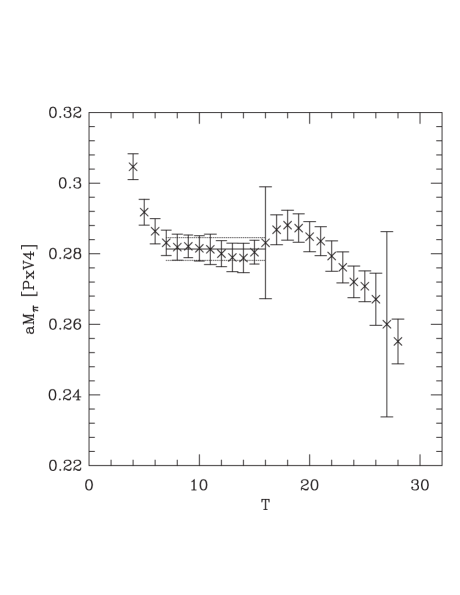
Figure 1: Effective pion mass for the three-link LT pion, $am_{\pi}(\gamma_{5}\otimes\xi_{4})$, for HYP-smeared staggered fermions, cubic U(1) sources (at $t=0$), and HPC sinks. The fit is discussed in the text. Based on 370 quenched gauge configurations ($\beta=6$), and using $m_{1}=m_{2}=0.03$ (corresponding to a particle with mass similar to that of the physical kaon).

The effective mass $m_{1}(t)$ is obtained by equating the form (12) to the lattice data for times $t-(t+3)$. The result of a fit to the range $7\leq t\leq 16$ is also shown. A good plateau is seen, with errors of $\approx 1.4\%$. Note that this is a “three-link” pion (quark and antiquark separated by three spatial links), which typically has the poorest signal of the LT tastes.

For pions with NLT tastes, our sources and sinks have different spins, and consequently the correlation functions have negative time-reflection parity. The appropriate fitting function is thus

$$f_{-}(t) = Z_{1}[\exp(-m_{1}t)\!-\!\exp(-m_{1}(L_{t}\!-\!t))]$$

$$+ Z_{2}(-1)^{t}[\exp(-m_{2}t)\!-\!\exp(-m_{2}(L_{t}\!-\!t))]\,.$$

An example of the corresponding effective mass is shown in Fig. 2. There is a reasonable plateau, but with errors of $\approx 3\%$ that are larger than those in Fig. 1. We note that this is the pion whose bilinear is the most non-local (involving three spatial links as well as the time link) and thus has the poorest signal.

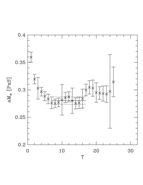
Figure 2: Effective mass for four-link NLT pion, $am_{\pi}(\gamma_{5}\otimes 1)$. Parameters are the same as in Fig. 1.

IV Quenched pion spectrum with unimproved staggered fermions

parameter	value
gauge action	Wilson plaquette action
# of sea quarks	0 (quenched QCD)
$\beta$	6.0
$1/a$	1.95 GeV (set by $\rho$ meson mass)
geometry	$16^{3}\times 64$
# of confs	370
gauge fixing	Coulomb
bare quark mass ($am_{q}$)	0.005, 0.01, 0.015, 0.02, 0.025, 0.03
$Z_{m}$	$\approx 2.5$

Table 1: Simulation parameters for quenched study of unimproved staggered fermions.

We begin with our results for unimproved staggered fermions on quenched lattices. Although, as described in the introduction, unimproved staggered fermions are not useful for most practical applications, we begin with them because they provide the benchmark against which improvements can be measured. Furthermore, we can test our methods of calculating the pion spectrum by comparing some of our results to those in the literature. A final motivation is that we are able to add new information by calculating with a wider range of quark masses than used previously.

The simulation parameters are given in Table 1. Here $Z_{m}$ is the factor by which the bare quark masses must be multiplied to obtain the renormalized mass in the $\overline{\rm MS}$ scheme at a scale of $2\;$GeV. We have only calculated the spectrum for equal quark and anti-quark masses, and only consider flavor non-singlet pions (so that there are no quark-disconnected contractions). To set the scale, we note that $am=0.025$ corresponds approximately to the physical kaon mass.

For $am=0.01$ and $0.02$, we can compare our results to those of Ref. ref:tsukuba , where the complete pion spectrum was calculated using similar methods.

	Ref. ref:tsukuba		This work
Operator	$am=0.01$	$am=0.02$	$am=0.01$	$am=0.02$
$(\gamma_{5}\otimes\xi_{5})$	0.23877(98)	0.33476(82)	0.2430(11)	0.3382(9)
$(\gamma_{5}\otimes\xi_{i5})$	0.2896(14)	0.3800(12)	0.2937(25)	0.3835(16)
$(\gamma_{5}\otimes\xi_{i4})$	0.3056(16)	0.3933(14)	0.3104(27)	0.3967(21)
$(\gamma_{5}\otimes\xi_{4})$	0.3167(20)	0.4016(16)	0.3230(48)	0.4061(28)
$(\gamma_{5}\otimes I)$	0.3300(46)	0.4110(26)	0.3323(57)	0.4127(40)
$(\gamma_{5}\otimes\xi_{45})$	0.2922(30)	0.3826(18)	0.2978(62)	0.3866(35)
$(\gamma_{5}\otimes\xi_{ij})$	0.3085(26)	0.3957(18)	0.3108(46)	0.3980(33)
$(\gamma_{5}\otimes\xi_{i})$	0.3168(33)	0.4026(19)	0.3211(49)	0.4061(38)

Table 2: Comparison of results for $(am_{\pi})$ with unimproved staggered fermions with those from Ref. ref:tsukuba . Our results are those with Golterman sink operators and cubic wall sources.

The comparison is shown in Table 2. Our results are systematically higher, although for most pions the difference is only $1-2\sigma$. For the Goldstone, taste $\xi_{5}$ pion, however, the difference is larger, $\sim 3-4\sigma$. These differences could be due to the details of fitting (our fitting range starts at somewhat later times), and they could at least in part indicate a finite volume effect (our lattices are smaller: $16^{3}\times 64$ versus $20^{3}\times 40$). In any case, we consider the agreement good enough for the subsequent discussion of taste-breaking effects.

As a test of our methods, it is also interesting to compare the relative size of our errors to those of Ref. ref:tsukuba . The errors are comparable for the Goldstone pion, while ours grow more quickly with the distance between quark and antiquark in the bilinears. We both use Coulomb-gauge sinks (although time-directed links are treated differently), so the differences between the calculations are the number of configurations (370 for us, versus 50), spatial volume (ours is half the size), and number and type of sources (Ref. ref:tsukuba uses one wall-source per color, and thus three times as many per configuration as we use). We speculate that the latter difference, and in particular the lack of noise from the U(1) sources, is responsible for the smaller errors of Ref. ref:tsukuba .

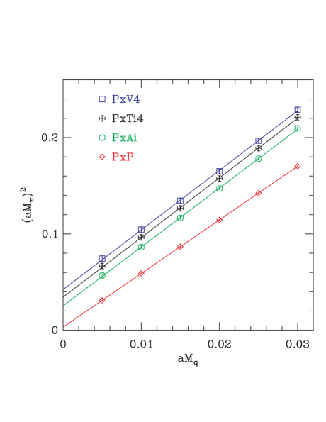
Figure 3: $(am_{\pi})^{2}$ vs. $am_{q}$ for unimproved quenched staggered fermions, with cubic wall sources and Golterman sinks. Only LT tastes are shown. Solid lines give the results of linear fits to the quark-mass dependence.

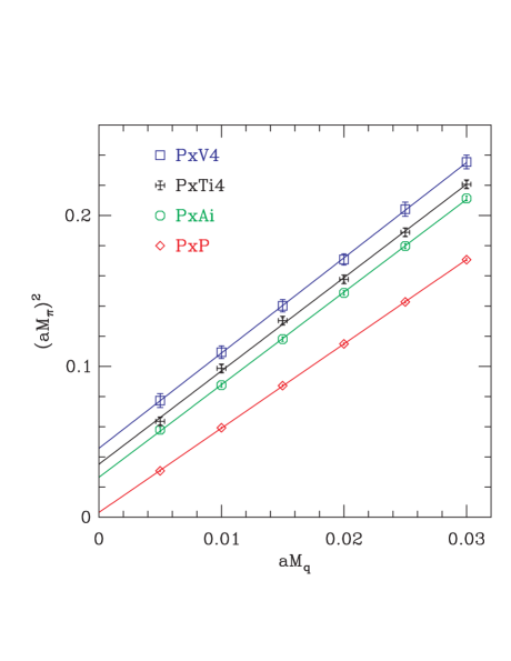
Figure 4: As for Fig. 3 except using cubic U(1) sources.

We show the comparison of the two sources for LT pions in Figs. 3 and 4, and for NLT pions in Figs. 5 and  6. In both cases the results from the two sources are consistent. We note, however, that the cubic wall sources lead to noticeably smaller errors for NLT pions than the cubic U(1) sources, although there is no such difference for LT pions.

Figure 5: $(am_{\pi})^{2}$ vs. $am_{q}$ for NLT tastes using unimproved quenched staggered fermions, with cubic wall sources and Golterman sinks. Solid lines give the results of linear fits to the quark-mass dependence.

Figure 6: As for Fig. 5 except with cubic U(1) sources.

We show results with HPC sinks (and cubic wall sources) in Figs. 7 and 8. Comparing these with Figs. 3 and 5, respectively, we see that the choice of sinks has no significant impact on the signal. (This is shown in more detail for HYP fermions below.) Thus we conclude that the extra irreps coupled to by the HPC sources do not significantly degrade the signal. Nevertheless, all else being equal, we prefer the Golterman sources.

We now turn to the nature of the taste breaking with unimproved fermions. Having results for all the tastes over a range of relatively light quark masses (down to $\approx m_{s}^{\rm phys}/5$) allows us to disentangle the different contributions. We note that the splittings are comparable to the pion mass-squareds themselves at the lightest quark masses, indicating that the appropriate power-counting is ${\cal O}(a^{2})\approx{\cal O}(p^{2})$. As seen in previous studies, the states are ordered according to the number of gauge-links traversed when moving between quark and anti-quark fields in the bilinear, although the splittings are not directly proportional to this number. In addition, we clearly observe that the slopes differ between the tastes: the splittings all increase with $m_{\pi}^{2}$, with almost a factor of two increase between the chiral limit and $am=am_{s}^{\rm phys}\approx 0.025$. (The values of the slopes for LT tastes are given in Table 6 below.) This difference in slopes arises at ${\cal O}(a^{2}p^{2})$ in chiral power-counting, and thus is a next-to-leading-order (NLO) effect. We thus expect it to be a small correction for our lightest quark masses, increasing to a significant correction for $m\approx m_{s}^{\rm phys}$. This is indeed what we find.

Staggered chiral perturbation theory predicts that the NLO contributions to the slopes for the four different LT tastes are independent ref:RuthSS . In fact, the numerical results tell us that the slopes for the heavier three tastes are consistent with each other, while being significantly larger than that for the Goldstone pion. This implies that some of the coefficients in the NLO staggered chiral Lagrangian are significantly smaller than others.

Another NLO prediction is that SO(4) taste symmetry should be broken, i.e. that the leading order (LO) degeneracy between tastes $A_{i}$ and $A_{4}$, $T_{i4}$ and $T_{ij}$, and $V_{4}$ and $V_{i}$, will no longer hold. The splitting is caused by terms of ${\cal O}(a^{2}p^{2})$, and thus affects only the slopes $(am_{\pi})^{2}/(am_{q})$, and not the intercepts ref:RuthSS . The difference in slopes within SO(4) irreps is predicted to be of the same order as that between SO(4) irreps. Taken at face value, this would imply that the SO(4) symmetry would be completely broken at the point that NLO contributions approach the size of those of LO (which, as we have seen, occurs at the upper end of our mass range).

In fact, we find no such breakdown in the SO(4) symmetry. The accuracy to which this symmetry holds can be seen most easily from Table 2, and also by comparing Figs. 7 and 8 (the points with the same colors in the two figures live in the same SO(4) multiplet). The errors for NLT tastes, while larger than for the LT tastes, are small enough that we can rule out a scenario with complete breakdown of SO(4) symmetry for our largest quark masses. In fact, our results are consistent with SO(4) symmetry for all quark masses. Thus we conclude that our results are consistent with the prediction of no SO(4) breaking in the intercepts, and that the coefficients of the SO(4) breaking in the slopes must be much smaller than the generic size.

Figure 7: $(am_{\pi})^{2}$ vs. $am_{q}$ for LT tastes using unimproved quenched staggered fermions, with cubic wall sources and HPC sinks.

Figure 8: As for Fig. 7 except for NLT pions.

V Quenched pion spectrum with HYP-smeared staggered fermions

parameter	value
gauge action	Wilson plaquette action
# of sea quarks	0 (quenched QCD)
$\beta$	6.0
$1/a$	1.95 GeV (set by $\rho$ meson mass)
geometry	$16^{3}\times 64$
# of confs	370
gauge fixing	Coulomb
smearing method	HYP (II) of Ref. ref:wlee:2
bare quark mass ($am_{q}$)	0.01, 0.02, 0.03, 0.04, 0.05
$Z_{m}$	$\approx 1$

Table 3: Simulation parameters for the quenched study with HYP-smeared staggered fermions.

	HPC		Golterman
Operator	CU1	CW	CU1	CW
$(\gamma_{5}\otimes\xi_{5})$	0.2262(27)	0.2261(26)	0.2263(27)	0.2267(35)
$(\gamma_{5}\otimes\xi_{i5})$	0.2313(27)	0.2311(31)	0.2314(30)	0.2302(26)
$(\gamma_{5}\otimes\xi_{i4})$	0.2355(29)	0.2348(32)	0.2356(29)	0.2339(27)
$(\gamma_{5}\otimes\xi_{4})$	0.2395(30)	0.2375(31)	0.2396(31)	0.2374(29)
$(\gamma_{5}\otimes\xi_{45})$	0.2293(74)	0.2239(69)	0.2343(72)	0.2239(69)
$(\gamma_{5}\otimes\xi_{ij})$	0.2338(77)	0.2264(56)	0.2346(79)	0.2233(61)
$(\gamma_{5}\otimes\xi_{i})$	0.2392(79)	0.2281(56)	0.2409(65)	0.2262(58)
$(\gamma_{5}\otimes I)$	0.2407(83)	0.2298(62)	0.2403(84)	0.2309(65)

Table 4: Source and sink dependence of $(am_{\pi})$. Results using HYP-smeared staggered fermions at $am=0.02$ on the quenched lattices. HPC and Golterman denote the choice of sink, while CU1 and CW denote cubic U(1) and cubic wall sources, respectively.

Using the same set of quenched gauge configurations as in Sec. IV, we now study the pion spectrum with HYP-smeared staggered fermions. The parameters we use are summarized in Table 3. We recall that HYP smearing is straightforward to implement in practice: one simply applies HYP smearing to the gauge configuration and then calculates the propagators using the unimproved staggered action on the resulting lattice. HYP smearing is carried out after Coulomb gauge fixing.

Despite using larger bare quark masses, our calculations with HYP-smeared fermions correspond to physical quarks which are slightly lighter than those used for unimproved staggered fermions in the previous section. This is because $Z_{m}\approx 1$ for HYP-smeared staggered fermions, whereas $Z_{m}\approx 2.5$ for unimproved staggered fermions. In particular, the physical strange quark mass is $am_{s}^{\rm phys}\approx 0.052$, slightly larger than our largest quark mass ref:wlee:BK , whereas the physical strange quark mass for unimproved fermions is approximately equal to the next-to-largest quark mass in that calculation ($am_{q}=0.025$).

Table 4 shows the dependence of pion masses on source and sink type for one choice of quark mass. As for unimproved quarks, the sink choice is unimportant (the central values are consistent, and the errors are very similar). It also remains true that the cubic wall sources lead to smaller errors for the NLT pions, although the reduction in the errors is a much smaller effect. While we do not understand why this is, it does mean that, in practice, the choice of source appears less crucial for HYP-smeared staggered fermions.

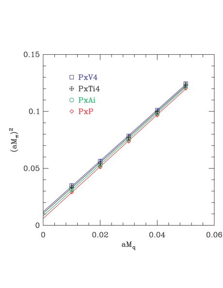
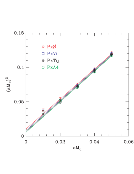
Figure 9: $(am_{\pi})^{2}$ vs. $am_{q}$ for HYP-smeared staggered fermions in quenched QCD, with cubic wall sources and Golterman sinks. Linear fits to the quark-mass dependence are shown. The left panel shows LT tastes; the right panel shows NLT tastes.

Taste ($F$)	$\Delta_{F}$ (unimproved)	$\Delta_{F}$ (HYP)
$\xi_{i5}$	0.0233(14)	0.0025(11)
$\xi_{i4}$	0.0320(27)	0.0050(14)
$\xi_{4}$	0.0425(49)	0.0073(13)
$\xi_{45}$	0.0244(91)	0.0036(53)
$\xi_{ij}$	0.0296(73)	0.0050(51)
$\xi_{i}$	0.0303(78)	0.0076(47)
$I$	0.0511(147)	0.0078(56)

Table 5: Comparison of taste symmetry breaking between unimproved and HYP-smeared fermions. Here $\Delta_{F}=[am_{\pi}(F)]^{2}-[am_{\pi}(\xi_{5})]^{2}$, extrapolated to the chiral limit. Both results are obtained using Golterman sinks and cubic U(1) sources in quenched QCD at $\beta=6.0$.

The resulting pion mass-squareds are shown for our preferred source and sink, and for all tastes, in Fig. 9. Comparing to the previous figures, we see that taste-breaking is substantially reduced. A quantitative measure of this is given in Table 5, which collects the mass-squared splittings after linear extrapolation to the chiral limit, both for the HYP and the unimproved action. Note that this measure is insensitive to the particular range of quark masses chosen (as long as they are small enough that linear fits work well). For the LT tastes, where the splittings with the HYP action are statistically significant, we find that HYP smearing reduces the splittings by a factor of $5-10$. The ordering of states is unchanged. For the NLT tastes, the splittings are reduced by similar factors, but the errors are large enough that a more quantitative statement cannot be made. For the same reason, we cannot make any quantitative comments on the size of possible SO(4) splitting.

Our results for the reduction in taste-breaking are qualitatively consistent with those obtained previously ref:hyp:1 ; ref:orginos:1 ; ref:mason:1 (although differences in simulation details do not allow a quantitative comparison). Having the results for a range of quark masses allows us to draw some conclusions on the appropriate power-counting. In particular, given the smallness of the splittings, it may be appropriate for this range of quark masses to treat the these ${\cal O}(a^{2})$ effects as of NLO rather than of LO, i.e. to assume that $a^{2}\sim p^{4}\sim m_{q}^{2}$.

Taste ($F$)	$c_{2}$ (unimproved)	$c_{2}$ (HYP)
$\xi_{5}$	5.57(2)	2.28(4)
$\xi_{i5}$	6.08(4)	2.26(4)
$\xi_{i4}$	6.03(9)	2.24(4)
$\xi_{4}$	5.99(10)	2.24(4)

Table 6: Comparison of taste symmetry breaking in slopes between unimproved and HYP-smeared fermions. $c_{2}$ is defined by fitting the data to $[am_{\pi}(F)]^{2}=c_{1}+c_{2}(am_{q})$. Both results are obtained using Golterman sinks and cubic wall sources in quenched QCD at $\beta=6.0$.

A test of this idea is provided by the taste-dependence of the slopes in the $m_{\pi}^{2}$ vs. $m_{q}$ plots. As noted in the previous section, this difference is an ${\cal O}(a^{2}p^{2})$ effect, and thus of NLO in the standard power counting of staggered chiral perturbation theory. It is observed at the expected order of magnitude with unimproved staggered fermions (see, e.g., Fig. 3). If the power-counting changes to $a^{2}\sim p^{4}$ for HYP-smeared fermions then the difference in the slopes would be of NNLO (next to next to leading order), and thus expected to be very small for our range of quark masses. This is indeed what we find. Table 6 collects the slopes for the LT tastes, and we see that, with HYP-smeared fermions, they are equal for all tastes within the statistical uncertainty, which is at the 2% level.

VI Comparison of asqtad and HYP-smeared staggered fermions

parameter	value
gauge action	1-loop tadpole-improved Symanzik
sea quarks	$2+1$ flavors of asqtad staggered
sea quark masses	$am_{\ell}=0.01$, $am_{s}=0.05$
$\beta$	6.76
$a$	0.125 fm
geometry	$20^{3}\times 64$
# of confs	640 (asqtad)/ 671 (HYP)
gauge fixing	Coulomb
valence quark type	asqtad and HYP staggered
valence quark mass (asqtad)	0.007, 0.01, 0.02, $\ldots$, 0.05
valence quark mass (HYP)	0.005, 0.01, 0.015, $\ldots$, 0.05
$Z_{m}$	$\approx 1$

Table 7: Simulation parameters used for the comparison of asqtad and HYP-smeared valence quarks. The HYP smearing uses the parameters of case (II) in Ref. ref:wlee:2 .

In this section we compare two types of improved staggered quark actions: the “asqtad” action used by the MILC collaboration and the HYP-smeared action. We use one of the so-called “coarse” lattice ensembles generated by the MILC collaboration ref:coarseMILC , with the average light quark mass roughly one fifth of the physical strange quark mass. The parameters of the study are summarized in Table 7. We note that the conventions of the asqtad action are such that, when comparing to the HYP action, the appropriate bare quark mass to use is $am_{q}/u_{0}$, where $u_{0}$ is the “average link” ref:milc:1 . In other words, if the HYP and asqtad quark masses are nominally equally, the HYP masses are actually smaller by a factor of $u_{0}=0.86774$ (this value coming from Ref. ref:milc:1 using one of the conventional definitions of $u_{0}$). To set the scale, the strange quark mass with the asqtad action is $\approx 0.045$, i.e. near the upper end of the range used, while that for the HYP action is $\approx 0.057$, which is somewhat above our heaviest quark mass. The results for asqtad valence quarks are from Ref. ref:milc:1 , while those for HYP-smeared quarks are new.

We only have results for HYP-smeared quarks using the cubic U(1) source. Although the results of the previous section indicate that this source is slightly inferior for NLT pions, our errors are small enough for the purposes of this study.

When we calculate HYP-smeared staggered quark propagators using the cubic U(1) source, we choose the source time slice randomly configuration by configuration such that unwanted autocorrelations in the two-point pion correlation functions are removed.

In Fig. 10, we show the results from Ref. ref:milc:1 for $(m_{\pi})^{2}$ for all tastes as a function of quark mass for asqtad valence quarks. This should be compared to our results with HYP-smeared valence fermions, given in Fig. 11 and Fig. 12. Note that different axes are used from the earlier plots, with the scale here being set by $r_{1}$, which is $2.61a$ on these lattices.

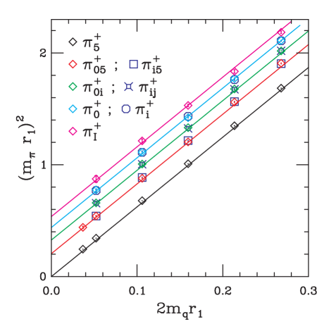
Figure 10: $(r_{1}m_{\pi})^{2}$ vs. $2r_{1}m_{q}$ on unquenched configurations, with asqtad valence quarks. All tastes are shown. The correspondence of the taste labels to those in other figures is as follows: $\pi_{5}\equiv\,$PxP, $\pi_{05}\equiv\,$PxA4, $\pi_{i5}\equiv\,$PxAi, $\pi_{0i}=\equiv\,$PxTi4, $\pi_{ij}\equiv\,$PxTij $\pi_{0}\equiv\,$PxV4, $\pi_{i}\equiv\,$PxVi, and $\pi\equiv\,$PxS. Results are from Ref. ref:milc:1 . The lines are linear fits to each taste.

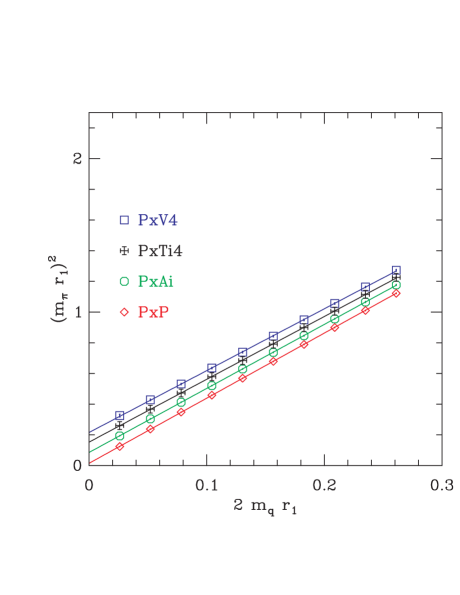
Figure 11: As for Fig. 10 for LT tastes except using HYP-smeared valence staggered fermions, with Golterman sinks and cubic U(1) sources.

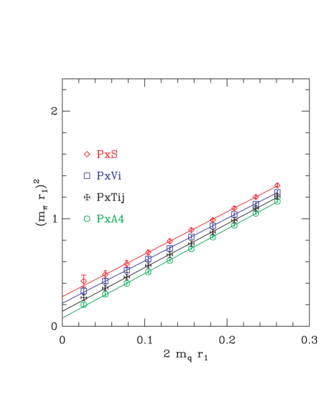
Figure 12: As for Fig. 10 for NLT tastes except using HYP-smeared valence staggered fermions, with Golterman sinks and cubic U(1) sources.

Comparing the two valence actions, we see that the taste-breaking is substantially reduced for HYP-smeared fermions. To make this quantitative we quote the values for some of the taste splittings, extrapolated to the chiral limit using linear fits, in Table 8. The splittings with HYP smearing are smaller by a factor of $2.5-3$. This is consistent qualitatively with the result noted in the introduction from Ref. ref:HISQ obtained on quenched lattices. It is also comparable to the factor of $3.6(5)$ improvement obtained using HISQ rather than asqtad fermions on similar dynamical lattices ref:HISQ .

Taste ($F$)	$\Delta_{F}$ (asqtad)	$\Delta_{F}$ (HYP)
$\xi_{i5}/\xi_{45}$	0.205(2)	0.0708(12)/0.062(13)
$\xi_{i4}/\xi_{ij}$	0.327(4)	0.1380(29)/0.125(16)
$\xi_{4}/\xi_{i}$	0.439(5)	0.2008(62)/0.199(26)
$I$	0.537(15)	0.257(34)

Table 8: Taste symmetry breaking effect: $\Delta_{F}=[r_{1}m_{\pi}(F)]^{2}-[r_{1}m_{\pi}(\xi_{5})]^{2}$ extrapolated to the chiral limit. Note that the scale is set here by $r_{1}$ and not the $1/a$ used earlier. Results from unquenched lattices comparing valence asqtad (from Ref. ref:milc:1 ) with HYP-smeared fermions (Golterman sinks with cubic U(1) sources).

A surprising feature of the comparison of Figs. 10 with Figs. 11 and 12 is that the slopes for the Goldstone pions differ: that for HYP-smeared fermions is about 1.4 times smaller than that for asqtad fermions. (The difference is emphasized by our use of the same vertical scales.) This slope is a parameter in the corresponding chiral Lagrangian, and should agree for the two actions up to differences in renormalization factors for the quark masses (aside from taste-conserving scaling violations). In fact, as already noted, the asqtad masses should be multiplied by $1/u_{0}\approx 1.15$, so that the horizontal scale in Fig. 10 should be stretched by a factor of 1.15, thus reducing the slope by this factor. This leaves a factor of about 1.2 difference in slopes to explain. This could be entirely due to differences in $Z_{m}$— the two-loop result for asqtad fermions is $Z_{m}\approx 1.16$ ref:mason , while that for the HYP action on asqtad sea-quarks is not known yet at one-loop. It is important to note, however, that the splittings given in Table 8 are in the chiral limit and thus are unaffected by any relative factors between the bare quark masses.

Returning to taste-breaking, we note that for both types of valence fermion the slopes for different tastes are nearly equal. For asqtad fermions we also see that no SO(4) breaking is apparent even at the largest quark masses (which, we recall, are close to the physical strange quark mass). Thus, despite the relatively large splittings with asqtad fermions [of ${\cal O}(a^{2})$ in the chiral counting], which are clearly to be treated as comparable to the contributions from the quark mass [of ${\cal O}(p^{2})$], there are no indications of NLO contributions [of ${\cal O}(a^{2}p^{2})$]. This is perhaps surprising and is in any case in contrast to unimproved staggered fermions where ${\cal O}(a^{2}p^{2})$ effects were clearly visible for a similar range of quark masses. For HYP-smeared fermions there is also no indication of NLO effects. The slopes are very close and, as can be seen from Table 8, there is no significant SO(4) breaking.

	quenched ($a\approx 0.1\;$fm)		unquenched ($a\approx 0.125\;$fm)
Taste($F$)	$\Delta_{F}$(unimproved)	$\Delta_{F}$(HYP)	$\Delta_{F}$(asqtad)	$\Delta_{F}$(HYP)
$\xi_{\mu 5}$	0.0931(56)	0.0094(41)	0.0759(7)	0.0262(5)
$\xi_{\mu\nu}$	0.128(11)	0.0189(53)	0.1211(14)	0.0511(11)
$\xi_{\mu}$	0.170(20)	0.0279(49)	0.1625(19)	0.0743(23)

Table 9: Comparison of taste-breaking for LT tastes on all lattices considered in this paper. $\Delta_{F}=[m_{\pi}(F)]^{2}-[m_{\pi}(\xi_{5})]^{2}$, now in units of ${\rm GeV}^{2}$.

We next compare taste-breaking for HYP-smeared fermions between the quenched lattices considered earlier and the dynamical lattices. Clearly, the splittings are significantly larger for the latter. To make this quantitative we compare the splittings in physical units in Table 9, where we see that they are 2-2.5 larger on the unquenched than on the quenched lattices with HYP-smeared fermions. Can we understand this? The answer is yes, at least qualitatively. Taste-breaking is expected to scale as $\alpha^{2}a^{2}$, since the contributions from one-gluon exchange have been removed. The lattice spacing on the dynamical lattices is larger, with the ratio of $a^{2}$ to that on the quenched lattices being about 1.5. We also know that $\alpha$ at a scale of $\approx 1/a$ (which is the scale relevant for taste-breaking gluon vertices) is larger on the dynamical lattices, since the long-distance physics has been (approximately) matched by construction, and the coupling runs toward zero more slowly for the dynamical lattices. Combining these effects, we expect to find that the taste-breaking for HYP-smeared fermions is perhaps twice as large on the dynamical as on the quenched lattices. This is in accord with our results. Note, however, that $\alpha^{2}a^{2}$ is reduced by about a factor of 2.5 between the MILC coarse and fine lattices ref:milc:1 . Thus we expect the taste-splitting on the MILC fine lattices with the HYP-action to be similar to that we observed above on the $a=1/10\;$fm quenched lattices.

In summary, the main difference between asqtad and HYP-smeared valence quarks is a substantial reduction in the LO taste-breaking splittings between SO(4) multiplets. Unlike the quenched case studied above, however, the power-counting $a^{2}\sim p^{2}$ appears to remain necessary on these coarse MILC lattices. It seems likely, however, that taste-breaking will be a NLO effect with HYP-smeared quarks on the fine MILC lattices.

VII Conclusion

In this paper, we have compared three versions of staggered fermions—unimproved, HYP-smeared, and asqtad—from the standpoint of taste-symmetry breaking. We confirm and make quantitative the hierarchy expected from previous work, namely that HYP smearing is significantly more effective at reducing taste-breaking than asqtad improvement. This is summarized in Table 9. Our results imply that HYP-smeared valence fermions on the fine MILC lattices (with $a\approx 1/11\;$fm) should have taste-breaking small enough that it will be possible to treat discretization errors as a NLO effect in chiral perturbation theory (rather than as a LO effect as required with asqtad fermions, and with HYP-smeared fermions on the coarse MILC lattices). This is an encouraging result for our ongoing calculations of electroweak matrix elements using HYP-smeared valence fermions.

To put the results into context, it is useful to convert the size of the splittings into a scale characterizing discretization errors. Taking the splitting of the 2-link LT pion (taste $\xi_{\mu\nu}$) as indicative of an “average” splitting, and setting $\Delta m_{\pi}^{2}=a^{2}\Lambda^{4}$, we find $\Lambda=0.5$ and $0.6\;$MeV for HYP fermions on the quenched and unquenched lattices, respectively. These are scales within the range of sizes that one would expect for generic discretization errors. In other words, the improvement due to HYP smearing brings the taste-breaking errors down into the range expected of generic discretization errors, so that discretization errors with staggered fermion are no longer anomalously large.

VIII Acknowledgments

Helpful discussions with A. Hasenfratz are acknowledged with gratitude. C. Jung is supported by the U.S. Dept. of Energy under contract DE-AC02-98CH10886. W. Lee acknowledges with gratitude that the research at Seoul National University is supported by the KICOS grant K20711000014-07A0100-01410, by the KRF grants (KRF-2006-312-C00497 and KRF-2007-313-C00146), and by the BK21 program of Seoul National University. The work of S. Sharpe is supported in part by the US Dept. of Energy grant DE-FG02-96ER40956. Computations for this work were carried out in part on facilities of the USQCD Collaboration, which are funded by the Office of Science of the U.S. Department of Energy.

Appendix A Anatomy of the hypercube operators

In Sec. III, we defined the hypercube operators, eq. (8), and noted that they are not irreps of the time-slice group of Ref. ref:golterman:1 . Here, following the procedure of Ref. ref:sharpe:2 , we express them in terms of true irreps. For simplicity, we work in the free theory, i.e. we do not explicitly include gauge links, but it is straightforward to add these at the end, following, say, the prescription in the text.

Consider a single hypercube operator of general spin and taste:

$$O^{\rm Klu}_{S,F}=\sum_{A,B}\bar{\chi}(A)(\overline{\gamma_{S}\otimes\xi_{F}})_{AB}\chi(B)\,.$$ (13)

Summing this over a timeslice as in eq. (8) leads to the HPC operators we actually use, but we delay this summation until necessary. To simplify the discussion, we first assume that $|S_{\mu}-F_{\mu}|=1$ for one index $\mu$, while $|S_{\nu}-F_{\nu}|=0$ for $\nu\neq\mu$. In other words, we first consider a “one-link” bilinear. We also need the “averaging” operator $\Phi_{\mu}$ given in eq. (11) and the derivative operator

$$D_{\mu}\chi(A) = \frac{1}{2}[\chi(A+\hat{\mu})-\chi(A-\hat{\mu})]\,,$$ (14)

in terms of which

$$\chi(A+\hat{\mu}) = \Phi_{\mu}\chi(A)+D_{\mu}\chi(A)$$ (15)

$$\chi(A-\hat{\mu}) = \Phi_{\mu}\chi(A)-D_{\mu}\chi(A)\,.$$ (16)

Now we can express the single-hypercube operator as (summation over $A,B$ now implicit)

$$O^{\rm Klu}_{S,F} = \bar{\chi}(A)(\overline{\gamma_{S}\otimes\xi_{F}})_{AB}(\delta_{B_{\mu},A_{\mu}+1}+\delta_{B_{\mu},A_{\mu}-1})\chi(B)$$

$$= \frac{1}{2}\bar{\chi}(A)(\overline{\gamma_{S}\otimes\xi_{F}})_{AB}\delta_{B_{\mu},A_{\mu}+1}[\Phi_{\mu}\chi(A)+D_{\mu}\chi(A)]$$

$$+ \frac{1}{2}[\Phi_{\mu}\bar{\chi}(B)-D_{\mu}\bar{\chi}(B)]\delta_{A_{\mu},B_{\mu}-1}(\overline{\gamma_{S}\otimes\xi_{F}})_{AB}\chi(B)$$

$$+ \frac{1}{2}\bar{\chi}(A)(\overline{\gamma_{S}\otimes\xi_{F}})_{AB}\delta_{B_{\mu},A_{\mu}-1}[\Phi_{\mu}\chi(A)-D_{\mu}\chi(A)]$$

$$+ \frac{1}{2}[\Phi_{\mu}\bar{\chi}(B)+D_{\mu}\bar{\chi}(B)]\delta_{A_{\mu},B_{\mu}+1}(\overline{\gamma_{S}\otimes\xi_{F}})_{AB}\chi(B)$$

$$= \frac{1}{2}\bar{\chi}(A)(\overline{\gamma_{S}\otimes\xi_{F}})_{AB}[\Phi_{\mu}\chi(A)]$$

$$+ \frac{1}{2}[\Phi_{\mu}\bar{\chi}(B)](\overline{\gamma_{S}\otimes\xi_{F}})_{AB}\chi(B)$$

$$+ \frac{1}{2}\bar{\chi}(A)(\overline{\gamma_{\mu 5S}\otimes\xi_{\mu 5F}})_{AB}[D_{\mu}\chi(A)]$$

$$- \frac{1}{2}[D_{\mu}\bar{\chi}(B)](\overline{\gamma_{\mu 5S}\otimes\xi_{\mu 5F}})_{AB}\chi(B)$$

In the last step we have used the following result for spin-taste matrices, assuming $|S_{\mu}-F_{\mu}|=1$:

$$(\overline{\gamma_{S}\otimes\xi_{F}})_{AB}(B-A)_{\mu}=(\overline{\gamma_{\mu 5S}\otimes\xi_{\mu 5F}})_{AB}\,.$$ (17)

Now we reinstate the sum over spatial hypercubes. Then the following identity holds:

$$\sum_{\vec{n}}\bar{\chi}(A)(\overline{\gamma_{S}\otimes\xi_{F}})_{AB}[\Phi_{\mu}\chi(A)]$$

$$=\sum_{\vec{n}}[\Phi_{\mu}\bar{\chi}(B)](\overline{\gamma_{S}\otimes\xi_{F}})_{AB}\chi(B)$$

$$\equiv[\sum_{\vec{n}}\bar{\chi}(\overline{\gamma_{S}\otimes\xi_{F}})\chi]_{T}$$ (18)

where $[\cdots]_{T}$ indicates that this is part of an irrep of the timeslice group of Ref. ref:golterman:1 . In fact, if $\mu$ is a spatial index, the $[\cdots]_{T}$ part of the HPC operator is identical to the corresponding Golterman operator of eq. (9). If $\mu=4$, the operator in (18) transforms in the same irrep as the corresponding Golterman operator, although it is not identical.

To pick out the remaining parts of the HPC operator, we define, as in Ref. ref:sharpe:2

$$\sum_{\vec{n}}\bar{\chi}(\overline{\gamma_{\mu 5S}\otimes\xi_{\mu 5F}})\overleftrightarrow{D}_{\mu}\chi$$

$$\equiv\sum_{\vec{n}}\big{\{}\bar{\chi}(A)(\overline{\gamma_{\mu 5S}\otimes\xi_{\mu 5F}})_{AB}[D_{\mu}\chi(A)]$$

$$\hskip 12.0pt-[D_{\mu}\bar{\chi}(B)](\overline{\gamma_{\mu 5S}\otimes\xi_{\mu 5F}})_{AB}\chi(B)\big{\}}\,.$$ (19)

This also transforms as part of an irrep of the timeslice group [a different irrep from that in which the operator (eq. 18) transforms, unless $\mu=4$]. Thus we can express the HPC operator as a sum of two true representations:

$$\sum_{\vec{n}}O^{\rm Klu}_{S,F} = [\sum_{\vec{n}}\bar{\chi}(\overline{\gamma_{S}\otimes\xi_{F}})\chi]_{T}$$ (20)

$$+\frac{1}{2}\sum_{\vec{n}}\bar{\chi}(\overline{\gamma_{\mu 5S}\otimes\xi_{\mu 5F}})\overleftrightarrow{D}_{\mu}\chi$$

Note that for $\mu=4$ these two operators, while having different spin-taste, lie in the same irrep of the timeslice group. This is the standard “doubling” of states discussed in the text.

The extension to operators containing more than one link is straightforward. For example, for distance two operators (i.e. $|S_{\mu}-F_{\mu}|=|S_{\nu}-F_{\nu}|=1$ for $\mu\neq\nu$, and $|S_{\rho}-F_{\rho}|=0$ for $\rho\neq\mu\neq\nu$), we find:

$$\sum_{\vec{n}}O^{\rm Klu}_{S,F} = [\sum_{\vec{n}}\bar{\chi}(\overline{\gamma_{S}\otimes\xi_{F}})\chi]_{T}$$ (21)

$$+\frac{1}{2}\sum_{\vec{n}}\bar{\chi}(\overline{\gamma_{\mu 5S}\otimes\xi_{\mu 5F}})\overleftrightarrow{D}_{\mu}\Phi_{\nu}\chi$$

$$+\frac{1}{2}\sum_{\vec{n}}\bar{\chi}(\overline{\gamma_{\nu 5S}\otimes\xi_{\nu 5F}})\overleftrightarrow{D}_{\nu}\Phi_{\mu}\chi$$

$$+\frac{1}{4}\sum_{\vec{n}}\bar{\chi}(\overline{\gamma_{\mu\nu S}\otimes\xi_{\mu\nu F}})\overleftrightarrow{D}_{\mu}\overleftrightarrow{D}_{\nu}\chi\,.$$

Thus there are four irreps (all different if $\mu\neq 4\neq\nu$) contained in the HPC operator.

In general, the HPC operator includes the Golterman operator (or, if $|S_{4}-F_{4}|=1$, an operator in the same irrep) as the leading term as well as operators with derivatives having different spin-taste. One expects the latter to have a coupling to physical states suppressed by $\sim a\Lambda_{\rm QCD}$ for each derivative. A similar analysis holds for the cubic U(1) sources, while the cubic wall sources should produce only true irreps aside from the effects of using only a few noise vectors. One should also keep in mind that the symmetries are not completely implemented when one has a finite ensemble of gauge configurations, although we expect this effect to be smaller than the use of only one source-set per configuration. Thus we expect the contamination from coupling to states of unwanted spin-taste to be smallest for the combination “Golterman-wall”, followed by “Golterman-U(1)”, then “HPC-wall”, and finally “HPC-U(1)”. This is not, however, the only source of systematic problems. The coupling to excited states within the same irrep should be more significant for wall than for U(1) sources.

References

- (1) S. R. Sharpe, PoS LAT2006, 022 (2006) [arXiv:hep-lat/0610094].
- (2) A. Hasenfratz and F. Knechtli, Phys. Rev. D64 (2001) 034504, [hep-lat/0103029].
- (3) K. Orginos, D. Toussaint, and R.L. Sugar, Phys. Rev. D60 (1999) 054503, [hep-lat/9903032].
- (4) G.P. Lepage, Phys. Rev. D59 (1999) 074502, [hep-lat/9809157].
- (5) Weonjong Lee, Phys. Rev. D66 (2002) 114504, [hep-lat/0208032].
- (6) E. Follana et al. [HPQCD Collaboration], Phys. Rev. D 75, 054502 (2007) [arXiv:hep-lat/0610092].
-
(7)
K. Symanzik,
Commun. Math. Phys. 45, 79 (1975);
Nucl. Phys. B 226, 187 (1983). - (8) A. Hasenfratz, R. Hoffmann and S. Schaefer, JHEP 0705, 029 (2007) [arXiv:hep-lat/0702028].
- (9) Weonjong Lee and Stephen Sharpe, Phys. Rev. D66 (2002) 114501, [hep-lat/0208018].
- (10) Weonjong Lee and Stephen Sharpe, Phys. Rev. D68 (2003) 054510, [hep-lat/0306016].
- (11) Maarten Golterman, Nucl. Phys. B273 (1986) 663-676.
- (12) Weonjong Lee and Stephen Sharpe, Phys. Rev. D60 (1999) 114503, [hep-lat/9905023].
- (13) C. Aubin and C. Bernard, Phys. Rev. D68 (2003) 034014, [hep-lat/0304014].
- (14) Ruth S. Van de Water, Stephen R. Sharpe, Phys. Rev. D73 (2006) 014003, [hep-lat/0507012].
- (15) E. Follana et al., Nucl. Phys. B (Proc. Suppl.) 129 (2004) 384, [hep-lat/0406021]; Nucl. Phys. B (Proc. Suppl.) 129 (2004) 447 [hep-lat/0311004].
- (16) U. M. Heller, F. Karsch and B. Sturm, Phys. Rev. D 60, 114502 (1999) [arXiv:hep-lat/9901010].
- (17) M. Cheng, N. H. Christ, C. Jung, F. Karsch, R. D. Mawhinney, P. Petreczky and K. Petrov, Eur. Phys. J. C 51, 875 (2007) [arXiv:hep-lat/0612030].
- (18) T. Bae et al., PoS (LATTICE 2007) 089 (2007), [arxiv:0710.0017].
- (19) Weonjong Lee, PoS LAT2006, 015 (2006), [hep-lat/0610058].
- (20) T. Bae et al., PoS LAT2006, 166 (2006), [hep-lat/0610056].
- (21) R. Gupta, G. Guralnik, G. W. Kilcup and S. R. Sharpe, Phys. Rev. D 43, 2003 (1991).
- (22) D. Pekurovsky and G. Kilcup, Phys. Rev. D 64, 074502 (2001) [arXiv:hep-lat/9812019].
- (23) H. Kluberg-Stern et al., Nucl. Phys. B220 (1983) 447.
-
(24)
D. Daniel and T. D. Kieu,
Phys. Lett. B 175, 73 (1986).
D. Daniel and S. N. Sheard, Nucl. Phys. B 302, 471 (1988). - (25) M. F. L. Golterman and J. Smit, Nucl. Phys. B 255, 328 (1985).
- (26) N. Ishizuka, M. Fukugita, H. Mino, M. Okawa and A. Ukawa, Nucl. Phys. B 411, 875 (1994).
- (27) S. Aoki et al., Phys. Rev. D62, 094501 (2000). [atXiv:hep-lat/9912007].
- (28) S. R. Sharpe and R. S. Van de Water, Phys. Rev. D 71, 114505 (2005) [arXiv:hep-lat/0409018].
- (29) W. Lee, T. Bhattacharya, G. T. Fleming, R. Gupta, G. Kilcup and S. R. Sharpe, Phys. Rev. D 71, 094501 (2005) [arXiv:hep-lat/0409047].
- (30) C. Bernard, et al., Phys. Rev. D64 (2001) 054506,
- (31) C. Aubin et al., Phys. Rev. D70 (2004) 114501, [hep-lat/0407028].
- (32) Q. Mason et al., Phys. Rev. D73 (2006) 114501, [hep-ph/0511160].
- (33) S. Sharpe and A. Patel, Nucl. Phys. B417 (1994) 307, [hep-lat/9310004].