Nonlinear intraband tunneling of BEC in a cubic three-dimensional lattice

Abstract

The intra-band tunneling of a Bose-Einstein condensate between three degenerate high-symmetry $X$-points of the Brillouin zone of a cubic optical lattice is studied in the quantum regime by reduction to a three-mode model. The mean-field approximation of the deduced model is described. Compared to the previously reported two-dimensional (2D) case [Phys. Rev. A 75, 063628 (2007)], which is reducible to the two-mode model, in the case under consideration there exist a number of new stable stationary atomic distributions between the $X$-points and a new critical lattice parameter. The quantum collapses and revivals of the atomic population dynamics are absent for the experimentally realizable time span. The 2D stationary configurations, embedded into the 3D lattice, turn out to be always unstable, while existence of a stable 1D distribution, where all atoms populate only one $X$-state, may serve as a starting point in the experimental study of the nonlinear tunneling in the 3D lattice.

I Introduction

In recent paper SK it has been shown that exploring the nonlinear tunneling of a Bose-Einstein condensate (BEC) loaded in a two-dimensional (2D) optical lattice allows for theoretical and experimental study of diversity of fundamental issues of the nonlinear physics. Among them we mention the validity of the mean-field approximation (considered previously in Ref. meanfiled ), which was used in the study of the nonlinear tunneling BKK ; BKKS , the accuracy of the semi-classical (i.e. WKB) approximation, where the inverse number of atoms $1/N$ plays the role of the effective Planck constant (similar to the ideas reported in Ref. VA for a coupled two-mode model and in Ref. KonKev for the Bohr-Sommerfeld quantization rule), and the macroscopic manifestation of the quantum collapses and revivals – a pure quantum effect related to the discrete nature of quantum spectra revivals . The approach developed in Ref. SK was based on the energy degeneracy due to the rotational, more specifically C₄, symmetry of the lattice, where the modulationally stable Bloch states at the high-symmetry $X$-points were used (for either attractive BEC loaded in the first lowest band or repulsive BEC loaded in the second band). The modulational stability allows one to reduce the mean-field description of spatially inhomogeneous matter waves to the effective two-mode model describing the populations of the resonant states (see also BK and the references therein). It was shown in Ref. BKKS by direct numerical simulations that the two-mode model gives a remarkably well description of the dynamics for a relatively long interval of time.

Since optical lattices are routinely available in all dimensions (see, for instance, the recent review 3Dlattice ), an intriguing possibility is to explore the dynamics similar that reported in Ref. SK but in the 3D case. Considering a cubic lattice one expects the dynamics to be much richer as compared to the 2D case, because the distinct X-points of the same band are now three-fold degenerate. Concentrating on the modulationally stable case, the only situation considered in the present paper, one would expect that the stable distributions are very different from those in the 2D configuration, moreover, the latter (embedded in the 3D lattice) is found to be unstable. The most significant feature of the problem at hand is that it reduces to an effective three-mode model, whose dynamics is described by a Hamiltonian with two degrees of freedom, due to the constraint imposed by conservation of the number of atoms. Taking into account that such dynamics in the vicinity of a stable point is, generally speaking, characterized by two frequencies, as well as the facts that in most of the spectrum the energy level spacing in the quantum model scales at least as $N^{-2}$ (except, for example, the local bound states close to the semiclassical stationary points) and that the number of atoms used in BEC experiments is large, one can expect that the phenomenon of quantum collapses and revivals in the respective quantum system is significantly affected (and even suppressed completely). At the same time new features can be expected due to the fact that the classical motion now can be either regular (in the vicinity of the stationary points) or chaotic, what will naturally affect the underlying quantum evolution.

Study of the phenomena mentioned above with special attention payed to the correspondence between quantum and semi-classical dynamics (like in the 2D case, the semi-classical dynamics will be obtained in the mean-field approach) constitutes the main goal of the present paper.

More specifically, we start by introducing in Sec. II the quantum model and discussing its validity, physical parameters and the time span achievable in possible experiments. The mean-field limit is derived in Sec. III by making use of the WKB approximation for the quantum model rewritten as a Schrödinger equation for an effective quantum particle. We study the stationary points of the mean-field dynamics and their stability by locally diagonalizing the Hamiltonian. In Sec. IV we compare the numerical simulations of the quantum model to those of the mean-field approach. Finally, in Sec. V we summarize the results.

II The reduced quantum model

II.1 The reduced Hamiltonian

Let us start with the Hamiltonian of a BEC in an optical lattice

$$H=\int\limits_{\mathcal{V}}\mathrm{d}^{3}{\bf x}\psi^{\dagger}({\bf x})\left(-\frac{\hbar^{2}}{2m}\nabla^{2}+V({\bf x})\right)\psi({\bf x})$$

$$+\frac{g}{2}\int\limits_{\mathcal{V}}\mathrm{d}^{3}{\bf x}\psi^{\dagger}({\bf x})\psi^{\dagger}({\bf x})\psi({\bf x})\psi({\bf x}),$$ (1)

where ${\bf x}\in\mathbb{R}^{3}$, $V({\bf x})$ is the cubic optical lattice potential, $\mathcal{V}=Mv_{0}$ is the total volume of the lattice consisting of $M$ cells each one of the volume $v_{0}$, $g$ is the interaction coefficient, and $\psi^{\dagger}({\bf x})$ and $\psi({\bf x})$ are the creation and annihilation field operators. Introducing the Bloch waves $\varphi_{n{\bf k}}({\bf x})$ through the standard eigenvalue problem

$$\left(-\frac{\hbar^{2}}{2m}\nabla^{2}+V({\bf x})\right)\varphi_{n{\bf k}}=E_{n{\bf k}}\varphi_{n{\bf k}},$$

where $n$ is a number of the zone and ${\bf k}$ is the wave-vector in the first Brillouin zone (BZ), we expand

$$\psi({\bf x})=\sum_{n,{\bf k}}\varphi_{n,{\bf k}}({\bf x})b_{n,{\bf k}},$$ (2)

where the creation and annihilation operators satisfy the usual commutation relations $[b_{n{\bf k}},b_{n^{\prime}{\bf k}^{\prime}}]=0$ and $[b_{n{\bf k}},b^{\dagger}_{n^{\prime}{\bf k}^{\prime}}]=\delta_{nn^{\prime}}\delta_{{\bf k}{\bf k}^{\prime}}$. The expansion (2) allows one to rewrite the Hamiltonian (1) in the form

$$H=\sum_{n,{\bf k}}E_{n{\bf k}}b^{\dagger}_{n{\bf k}}b_{n{\bf k}}+$$

$$\sum_{{\bf k}_{1},...,{\bf k}_{4}\atop n_{1},...,n_{4}}\chi^{n_{1}n_{2}n_{3}n_{4}}_{{\bf k}_{1}{\bf k}_{2}{\bf k}_{3}{\bf k}_{4}}\delta_{{\bf k}_{1}+{\bf k}_{2}-{\bf k}_{3}-{\bf k}_{4},{\bf Q}}b^{\dagger}_{n_{1}{\bf k}_{1}}b^{\dagger}_{n_{2}{\bf k}_{2}}b_{n_{3}{\bf k}_{3}}b_{n_{4}{\bf k}_{4}},$$

(3)

where ${\bf Q}$ is an arbitrary vector of the reciprocal lattice and

$$\chi^{n_{1}n_{2}n_{3}n_{4}}_{{\bf k}_{1}{\bf k}_{2}{\bf k}_{3}{\bf k}_{4}}=\frac{g}{2}\int\limits_{\mathcal{V}}\mathrm{d}^{2}{\bf x}\varphi^{*}_{n_{1}{\bf k}_{1}}\varphi^{*}_{n_{2}{\bf k}_{2}}\varphi_{n_{3}{\bf k}_{3}}\varphi_{n_{4}{\bf k}_{4}}$$ (4)

(hereafter the asterisk stands for the complex conjugation).

By analogy with the 2D case SK , after the symmetry of the lattice is fixed the nonlinear tunneling phenomenon in 3D does not depend on the particular shape of the potential, as for instance on its separability: the only lattice parameter $\Lambda$ entering the model, see Eq. (12) below, characterizes the effective lattice depth rather than its geometric properties. Therefore we concentrate on the simplest case of a separable cubic lattice:

$$V=sE_{r}[\cos(x/\mathrm{d})+\cos(y/\mathrm{d})+\cos(z/\mathrm{d})],$$ (5)

where $\mathrm{d}$ is the lattice period and the lattice depth $s$ is measured in the units of the recoil energy $E_{r}=\hbar^{2}\pi^{2}/(2md^{2})$. The respective BZ is given by $[-\frac{\pi}{\mathrm{d}},\frac{\pi}{\mathrm{d}}]\times[-\frac{\pi}{\mathrm{d}},\frac{\pi}{\mathrm{d}}]\times[-\frac{\pi}{\mathrm{d}},\frac{\pi}{\mathrm{d}}]$.

We consider the three distinct $X$-points, $X_{1}=(\frac{\pi}{d},0,0)$, $X_{2}=(0,\frac{\pi}{d},0)$ and $X_{3}=(0,0,\frac{\pi}{d})$, degenerate in the Bloch energy, which pertain to the modulationally stable Bloch band, and assume that only these points are significantly populated by the BEC atoms at $t=0$. Then, repeating the arguments of the 2D case SK it can be shown that for small $g$ (see also below) the energy and quasi-momentum conservation laws allow one to discard the transitions, due to the scattering of BEC atoms, to all other points except the transitions between the three degenerate $X$-points. We arrive at the three-mode approximation:

$$\psi({\bf x})=\varphi_{1}({\bf x})b_{1}+\varphi_{2}({\bf x})b_{2}+\varphi_{3}({\bf x})b_{3},$$ (6)

where the Bloch function $\varphi_{j}({\bf x})$ and the operator $b_{j}$ correspond to the $X_{j}$-point (here we use the simplified-index notations for the populated states). Substitution of this expression into Eq. (1) results in the approximate Hamiltonian

$$H_{X} = \sum_{j=1}^{3}\left(E_{X}b^{\dagger}_{j}b_{j}+\chi_{1}b_{j}^{\dagger}b_{j}^{\dagger}b_{j}b_{j}\right)$$ (7)

$$+ \chi_{2}\left(4\sum_{j<k}b_{j}^{\dagger}b_{k}^{\dagger}b_{j}b_{k}+\sum_{j\neq k}(b_{j}^{\dagger})^{2}(b_{k})^{2}\right)$$

where $E_{X}$ is the Bloch energy at the $X$-point and the only nozero coefficients (4) are given by

$$\chi_{1}=\frac{g}{2}\int\limits_{\mathcal{V}}\mathrm{d}^{3}{\bf x}\,|\varphi_{1}|^{4},\quad\chi_{2}=\frac{g}{2}\int\limits_{\mathcal{V}}\mathrm{d}^{3}{\bf x}\,|\varphi_{1}|^{2}|\varphi_{2}|^{2}.$$ (8)

The Hamiltonian (7) commutes with the total number of atoms $N$ in the $X$-points

$$\sum_{j=1}^{3}n_{j}=N,\quad n_{j}=b_{j}^{\dagger}b_{j}$$ (9)

which reflects the approximation made.

The details of the derivation can be found in Ref. SK . Let us, however, present an alternative way to arrive at the Hamiltonian (7). First we note that if initially only the $X$-points of the same Bloch band are populated, the rates of the quantum transitions to other points (within the same band and to other Bloch bands) due to the $s$-wave atomic scattering (i.e. the nonlinearity of BEC), treated as a perturbation, are defined, according to the Fermi golden rule, by the energy conservation between the initial and final states within the linear model and are proportional to the density of the states at the particular point to which the transition takes place. In our particular case, an additional rule on the transitions, satisfied by the nonlinearity of BEC, is that the sum of the quasi-momenta of the two atoms before the scattering and after that can differ only by some reciprocal lattice vector (we consider the Bloch waves as the basis). Recalling that the density of states is large only on the boundary of the Brillouin zone (it diverges in the limit of an infinite lattice) and only the $X$-points of the same Bloch band on the boundary have the same energy and satisfy the quasi-momentum conservation (in the above sense), all transitions except those to the $X$-points of the same band can be neglected. The same conclusion is also derived within the mean-field approach. Indeed, the resonant four-wave processes are determined by the phase-matching conditions (equivalent to the energy and the quasi-momentum conservation) and the population of the respective points, thus unpopulated points (or entire bands) which do not satisfy the matching conditions do not make any contribution to the resonant processes.

In this set of arguments, the transitions to other (resonant) points of the same Bloch band are neglected due to either the negligibly low density of states compared to that at the boundary points or due to the quasi-momentum non-conservation. On the other hand, the transitions to the boundary points of other Bloch bands are neglected due to the energy conservation, i.e. under the condition that the nonlinearity of BEC is much smaller than the band gap at the boundary of the Brillouin zone. In the shallow lattice limit $s\ll 1$ ($\Lambda$ close to 1), for instance, the condition of a relatively large gap requires that $\chi_{1}N\sim gN/{\cal V}\ll E_{r}$.

On the other hand, we use the expansion over the Bloch-wave basis [see Eq. (2)], what means that a few-mode approximation implies concentration of particles in the respective states. This imposes a constraint on the potential depth. Indeed, two body interactions result in nonzero spectral width of a Bloch state, which in our case can be estimated as $\omega_{NL}=\frac{4\chi_{1}N}{\hbar}$. In order to be able to neglect the effect of the spectral width on the dynamics (what is done in the present paper) one has to require it to be much less than the spectral width of the lowest band (the most narrow band in the general situation). The latter is typically of order of the recoil energy $E_{r}$. Thus we require $\omega_{NL}\ll E_{r}/\hbar$ (notice that that this is the limit in some sense opposite to the standard conditions of applicability of the Bose-Hubbard model, where due to relatively large amplitude of the periodic potential and, consequently, strong on-site localization of the wave functions, the expansion over Wannier functions is more appropriate). In order to get an idea about the physical range of the parameters, let us estimate the frequency $\omega_{NL}$. The coefficient $\chi_{1}=\frac{g}{2}\int\mathrm{d}x^{3}|\varphi|^{4}\sim\frac{g}{2\mathcal{V}}$, hence we can estimate

$$\omega_{NL}\sim\frac{8\pi\hbar a_{s}}{m}\frac{N}{\mathcal{V}}=\frac{1}{\gamma}\frac{a_{s}}{m}\frac{N}{\mathcal{V}},$$ (10)

$$\gamma=3.78\times 10^{32}(J\cdot s)^{-1}.$$

For instance, for ⁸⁷Rb we have $m=1.44\times 10^{-25}kg$ and $a_{s}=5.1nm$ thus for a lattice with $M=20^{3}$ cells with the lattice constant $d=1\mu m$ ($v_{0}=10^{-12}$cm³) and $N=1000$ we get $\omega_{NL}\sim 12.5Hz$. On the other hand assuming the potential depth to be equal to the recoil energy we obtain the width of the first lowest band to be $0.59\cdot E_{r}/\hbar\approx 590$ Hz, and thus $\hbar\omega_{NL}/E_{r}\approx 0.021$. By reducing the potential depth this relation can be further improved.

In this context it is also relevant to mention, that the dimensional time $\tau$ is measured in the units $1/\omega_{NL}$, which for the above example is approximately $0.08$ s. Taking into account that the characteristic lifetime of a condensate can reach $10s$, we conclude that for typical experiments the characteristic time is about $100$ dimensionless units. This time can be significantly enlarged (i.e. making observation of the reported effect much easier) by using lighter, say lithium, atoms and/or with a larger $s$-wave scattering length, achievable by Feshbach resonance.

II.2 The dynamical equations

It is convenient to use the dimensionless time $\tau=\omega_{NL}t$, subtract from the Hamiltonian (7) the constant term $H_{0}=(E_{X}-\chi_{1})N$ [here we use Eq. (9)] and normalize the result by dividing by $N^{2}$, which allows for the transition to the mean-field limit $N\to\infty$, since the resulting Hamiltonian is written in the population densities $n_{j}/N$. This results in the Schrödinger equation

$$\frac{i}{N}\partial_{\tau}|\Psi\rangle=\hat{H}|\Psi\rangle,$$ (11)

with the Hamiltonian

$$\hat{H}=\frac{1}{N^{2}}\left(\frac{1}{4}\sum_{j=1}^{3}n_{j}^{2}+\Lambda\sum_{j<k}n_{j}n_{k}+\frac{\Lambda}{4}\sum_{j\neq k}(b^{\dagger}_{j})^{2}b_{k}^{2}\right)\!,$$ (12)

where $\Lambda=\chi_{2}/\chi_{1}$. Equation (12) may be interpreted as a Schrödinger equation for a single quantum particle (see also Eq. (17) below).

Denoting by $k_{j}$ the number of atoms populating the X_j-point (such that $k_{1}+k_{2}+k_{3}=N$) one can expand the wave function $|\Psi\rangle$ over the Fock basis $|k_{1},k_{2},N-k_{1}-k_{2}\rangle\equiv|k_{1}\rangle|k_{2}\rangle|N-k_{1}-k_{2}\rangle$:

$$|\Psi\rangle=\sum_{k_{1}=0}^{N}\sum_{k_{2}=0}^{N-k_{1}}C_{k_{1},k_{2}}(t)|k_{1},k_{2},N-k_{1}-k_{2}\rangle,$$ (13)

where the expansion coefficients obey the normalization condition

$$\sum_{k_{1}=0}^{N}\sum_{k_{2}=0}^{N-k_{1}}|C_{k_{1},k_{2}}(t)|^{2}=1.$$ (14)

Now Eq. (12) can be cast in the form:

$$\frac{i}{N}\frac{dC_{k_{1},k_{2}}}{d\tau} = \frac{1}{4}a_{k_{1},k_{2}}C_{k_{1},k_{2}}+\frac{\Lambda}{4}\left(b_{k_{1}-1,k_{2}}C_{k_{1}-2,k_{2}}+b_{k_{1}+1,k_{2}}C_{k_{1}+2,k_{2}}+b_{k_{2}-1,k_{1}}C_{k_{1},k_{2}-2}+b_{k_{2}+1,k_{1}}C_{k_{1},k_{2}+2}\right.$$ (15)

$$+ \left.d_{k_{1}-1,k_{2}+1}C_{k_{1}-2,k_{2}+2}+d_{k_{1}+1,k_{2}-1}C_{k_{1}+2,k_{2}-2}\right),$$

where

$$a_{k_{1},k_{2}}=1+2(2\Lambda-1)N^{-2}\left[(k_{1}+k_{2})(N-k_{1}-k_{2})+k_{1}k_{2}\right],$$

$$b_{k_{1},k_{2}}=N^{-2}\left\{k_{1}(1+k_{1})(N-k_{1}-k_{2}+1)(N-k_{1}-k_{2})\right\}^{1/2},$$

$$d_{k_{1},k_{2}}=N^{-2}\left\{k_{1}(1+k_{1})k_{2}(1+k_{2})\right\}^{1/2}.$$

We notice that the coefficients are defined only for $0\leq k_{1}+k_{2}\leq N$, which is the lower left triangular part of the corresponding matrix representation and the coefficient $b_{k_{1},k_{2}}$ is not symmetric with respect to the exchange of the indexes.

The nonlinearity, though being responsible for the very existence of the intraband tunneling, only defines the time scale and it is the lattice parameter $\Lambda$ which enters the Hamiltonian in Eq. (12) ($\Lambda$ is a ratio of two integrals of the Bloch waves which are defined solely by the lattice).

We conclude this section with the estimate for the energy range:

$$\frac{1+2\Lambda}{12}+\frac{\Lambda}{2N}\leq\langle\hat{H}\rangle\leq\frac{1+2\Lambda}{4}-\frac{\Lambda}{2N},\;\Lambda\leq\frac{1}{4}$$

$$\frac{1-2\Lambda}{4}+\frac{\Lambda}{2N}\leq\langle\hat{H}\rangle\leq\frac{1+2\Lambda}{4}-\frac{\Lambda}{2N},\;\Lambda>\frac{1}{4},$$

(16)

(see Appendix A) important for the numerical simulations. Since the Hamiltonian (12) is bounded from above and from below it follows that the energy spacing for the quantum particle satisfying equation (11) is, for the most of the spectrum, on the order of $\delta E\sim N^{-2}$: for a given number of atoms $N$ the dimension of the Hilbert space is $(N+1)(N+2)/2$ i.e. $\approx N^{2}/2$ in the limit $N\ll 1$ (in the 2D case, considered in Ref. SK , the dimension of the respective Hilbert space was $N+1$ and respectively the energy distance between adjacent energy levels was determined by the factor $N^{-1}$).

III The semi-classical approximation

III.1 The governing dynamical model

The semi-classical approach employed here is similar to that of Ref. SK . We define $h=2/N$, $x_{1,2}=k_{1,2}/N$. Then, assuming existence of a regular function $\psi(x_{1},x_{2})\equiv\frac{N+1}{2}C_{k_{1},k_{2}}$, Eq. (15) is cast as

$$ih\partial_{\tau}\psi=\frac{1}{2}a(x_{1},x_{2})\psi+\frac{\Lambda}{2}\biggl{\{}b_{h}\left(x_{1}-\frac{h}{2},x_{2}\right)e^{-i\hat{p}_{1}}+b_{h}\left(x_{1}+\frac{h}{2},x_{2}\right)e^{i\hat{p}_{1}}+b_{h}\left(x_{2}-\frac{h}{2},x_{1}\right)e^{-i\hat{p}_{2}}$$

$$+b_{h}\left(x_{2}+\frac{h}{2},x_{1}\right)e^{i\hat{p}_{2}}+d_{h}\left(x_{1}-\frac{h}{2},x_{2}+\frac{h}{2}\right)e^{i(\hat{p}_{2}-\hat{p}_{1})}+d_{h}\left(x_{1}+\frac{h}{2},x_{2}-\frac{h}{2}\right)e^{i(\hat{p}_{1}-\hat{p}_{2})}\biggr{\}}\psi,$$

(17)

where $\hat{p}_{j}=-ih\partial_{x_{j}}$ and we have introduced the functions, defined on the triangular domain $0\leq x_{1}+x_{2}\leq 1$:

$$a(x_{1},x_{2})=1+2(2\Lambda-1)\left[b_{0}(x_{1},x_{2})+b_{0}(x_{2},x_{1})+d_{0}(x_{1},x_{2})\right],$$

$$b_{h}(x_{1},x_{2})=\left[x_{1}\left(x_{1}+\frac{h}{2}\right)\left(1-x_{1}-x_{2}\right)\left(1-x_{1}-x_{2}+\frac{h}{2}\right)\right]^{1/2},$$

$$d_{h}(x_{1},x_{2})=\left[x_{1}\left(x_{1}+\frac{h}{2}\right)x_{2}\left(x_{2}+\frac{h}{2}\right)\right]^{1/2}.$$

We have $[\hat{p_{j}},x_{k}]=-ih\delta_{j,k}$, i.e. the usual canonical commutator of the momenta and coordinates. Evidently, the rôle played by $h$ is of the effective Planck constant. The semi-classical dynamics corresponds to the limit $h\to 0$, i.e. when the number of BEC atoms $N\to\infty$. It is important to recall that the characteristic time $t$ of the evolution scales as $(\chi_{1}N)^{-1}\tau$, hence the quantity $\chi_{1}N$ must be kept fixed. These two conditions taken together constitute the usual mean-field limit for BEC. It is important to mention here that the coefficients $\chi_{1,2}$ stay bounded, as it follows form the definition (8) and the normalization of the wave function, implying $\int|\varphi_{j}|^{2}|\varphi_{k}|^{2}\sim 1/{\cal V}$. The quantity $\chi_{1}N\sim gN/{\cal V}$ giving the scale of the nonlinear time $T_{NL}=2\pi/\omega_{NL}$ (see Eq. (10)) is constant also in the thermodynamic limit defined as $N\to\infty$ at a constant density.

The limit $h\to 0$, if it exists, corresponds to the continuous limit of the discrete equation (17) (in this respect, it is similar to the WKB approach used for the discrete three-term relation, see Ref. braun for details).

In order to derive the classical equation corresponding to the limit $h\to 0$ we set $\psi(x_{1},x_{2},\tau)=e^{iS(x_{1},x_{2},\tau,h)/h}$ for a complex action $S(x_{1},x_{2},\tau,h)$ viewed as a series $S=S^{(0)}+hS^{(1)}+O(h^{2})$. Assuming the action $S^{(0)}(x_{1},x_{2},\tau)$ be differentiable function we get the Hamilton-Jacobi equation for the classical action $S^{(cl)}(x_{1},x_{2},\tau)=S^{(0)}(x_{1},x_{2},\tau)-\tau/2$:

$$-S^{(cl)}_{\tau} = b_{0}(x_{1},x_{2})\left[\Lambda\cos\left(S^{(cl)}_{x_{1}}\right)+2\Lambda-1\right]+b_{0}(x_{2},x_{1})\left[\Lambda\cos\left(S^{(cl)}_{x_{2}}\right)+2\Lambda-1\right]$$ (18)

$$+d_{0}(x_{1},x_{2})\left[\Lambda\cos\left(S^{(cl)}_{x_{1}}-S^{(cl)}_{x_{2}}\right)+2\Lambda-1\right]\equiv{\mathcal{H}}\left(S^{(cl)}_{x_{1}},S^{(cl)}_{x_{2}},x_{1},x_{2}\right),$$

where we have introduced the classical Hamiltonian $\mathcal{H}$. The quasi-classical dynamics is sometimes more conveniently described in terms of variables $z_{j}=1-2x_{j}$ and $\phi_{j}=\tilde{S}^{(cl)}_{x_{j}}=p$, where $x_{j}$ and $p_{j}$ are the classical limits of the corresponding quantum variables. The Poisson brackets of the respective classical variables read

$$\{\phi_{j},z_{k}\}=\lim_{h\to 0}\frac{i}{h}[\hat{p}_{j},1-2x_{k}]=-2\delta_{j,k},$$

$$\{\phi_{j},\phi_{k}\}=\{z_{j},z_{k}\}=0.$$ (19)

The classical variables can be associated with the quantum averages by the following correspondence:

$$z_{j} = 1-\frac{2}{N}\langle b_{j}^{\dagger}b_{j}\rangle=1-\frac{2}{N}\sum_{k_{1}=0}^{N}\sum_{k_{2}=0}^{N-k_{1}}k_{j}|C_{k_{1},k_{2}}|^{2},\quad$$ (20)

$$\phi_{1} = \mathrm{arg}\langle(b_{1}^{\dagger})^{2}b_{3}^{2}\rangle$$ (21)

$$= \mathrm{arg}\left\{\sum_{k_{1}=0}^{N}\sum_{k_{2}=0}^{N-k_{1}}C^{*}_{k_{1},k_{2}}b_{k_{1}+1,k_{2}}C_{k_{1}+2,k_{2}}\right\},$$

$$\phi_{2} = \mathrm{arg}\langle(b_{2}^{\dagger})^{2}b_{3}^{2}\rangle$$ (22)

$$= \mathrm{arg}\left\{\sum_{k_{1}=0}^{N}\sum_{k_{2}=0}^{N-k_{1}}C^{*}_{k_{1},k_{2}}b_{k_{2}+1,k_{1}}C_{k_{1},k_{2}+2}\right\}.$$

The first equalities in these formulae can be most easily established by replacement of the boson operators by $c$-numbers: $b_{j}^{\dagger}\to\sqrt{N}(b^{(cl)})^{*}$ and $b_{j}\to\sqrt{N}b^{(cl)}$. The phase difference $\phi_{j}$ in Eqs. (21)-(22) is not defined if $\langle b_{j}^{\dagger}b_{j}\rangle=0$, i.e. $z_{j}=1$ (the function “arg” in Eq. (21) or (22) is applied to zero: $C_{k^{\prime}_{1},k^{\prime}_{2}}=0$ for $k^{\prime}_{j}\geq 1$). The two phases are not defined also for $z_{1}+z_{2}=0$, i.e. $\langle b_{3}^{\dagger}b_{3}\rangle=0$, since in this case $b_{3}|\Psi\rangle=0$. In these cases the phases can be determined by taking the averages of the boson operators corresponding to non-zero average populations, i.e. in the semi-classical limit instead of $(b^{*}_{j}b_{k})^{2}$ one just takes the phase of the squared nonzero amplitude $b_{k}^{2}$ or $(b^{*}_{j})^{2}$.

The classical Hamiltonian, recovered from the Hamilton-Jacobi equation (18), reads

$$\mathcal{H}=\frac{1}{4}(1-z_{1})(z_{1}+z_{2})(\Lambda\cos\phi_{1}+2\Lambda-1)$$

$$+\frac{1}{4}(1-z_{2})(z_{1}+z_{2})(\Lambda\cos\phi_{2}+2\Lambda-1)$$

$$+\frac{1}{4}(1-z_{1})(1-z_{2})(\Lambda\cos(\phi_{1}-\phi_{2})+2\Lambda-1).$$ (23)

As a result of Eq. (19) the mean-field equations of motion acquire the form ($j=1,2$)

$$\frac{dz_{j}}{d\tau}=-2\frac{\partial\mathcal{H}}{\partial\phi_{j}},\qquad\frac{d\phi_{j}}{d\tau}=2\frac{\partial\mathcal{H}}{\partial z_{j}}.$$ (24)

Explicitly they read

$$\dot{z}_{1} = \frac{\Lambda}{2}(1-z_{1})[(z_{1}+z_{2})\sin\phi_{1}+(1-z_{2})\sin(\phi_{1}-\phi_{2})],$$ (25a)

$$\dot{z}_{2} = \frac{\Lambda}{2}(1-z_{2})\left[(z_{1}+z_{2})\sin\phi_{2}+(1-z_{1})\sin(\phi_{2}-\phi_{1})\right],$$ (25b)

$$\dot{\phi}_{1} = \frac{1}{2}(1-2z_{1}-z_{2})(\Lambda\cos\phi_{1}+2\Lambda-1)+\frac{\Lambda}{2}(1-z_{2})[\cos\phi_{2}-\cos(\phi_{1}-\phi_{2})],$$ (25c)

$$\dot{\phi}_{2} = \frac{1}{2}(1-2z_{2}-z_{1})(\Lambda\cos\phi_{2}+2\Lambda-1)+\frac{\Lambda}{2}(1-z_{1})[\cos\phi_{1}-\cos(\phi_{1}-\phi_{2})].$$ (25d)

III.2 Stationary points

Either from the point of view of dynamics governed by Eq. (25) or from the point of view of practical applications the most relevant first step in studying the mean-field dynamics is the investigation of stationary points $P_{j}=\{z_{1,j}^{(st)},z_{2,j}^{(st)},\phi_{1,j}^{(st)},\phi_{2,j}^{(st)}\}$ and of their stability. We emphasize that now the stability is understood in the classical mechanics sense, unlike the modulational instability of the Bloch states mentioned in the Introduction and resulting in developing of the spatial structures BKK ; BKKS ; BK .

We will use the notations $\zeta_{\alpha}=z_{\alpha}-z_{\alpha,j}^{(st)}$ and $\varphi_{\alpha}=\phi_{\alpha}-\phi_{\alpha,j}^{(st)}$ for local coordinates describing small deviations from the stationary solutions. The relation between the populations $x_{j}$ and dynamical variables $z$ reads

$$(x_{1},x_{2},x_{3})=\frac{1}{2}(1-z_{1},1-z_{2},z_{1}+z_{2}).$$ (26)

It is convenient to separate internal stationary points, i.e. the ones for which all three $X$-points are populated from the boundary stationary points for which either one or two $X$-points have zero population. The boundary stationary points correspond to the effectively low-dimensional (2D or 1D) distributions of atoms in the 3D lattice.

III.2.1 Internal stationary points

1. The first internal stationary point is given by $P_{1}=\left\{\frac{1}{3},\frac{1}{3},0,0\right\}$ and describes equally populated X-points with zero phases (phase differences). The Hamiltonian in the vicinity of $P_{1}$ reads

$$\mathcal{H}_{P_{1}} = \frac{1}{4}(1-3\Lambda)(\zeta_{1}^{2}+\zeta_{2}^{2}+\zeta_{1}\zeta_{2})$$ (27)

$$-\frac{\Lambda}{9}(\varphi_{1}^{2}+\varphi_{2}^{2}-\varphi_{1}\varphi_{2})-\frac{1}{3}.$$

It can be diagonalized using the generation function $F_{2}=(p_{1}+p_{2})\varphi_{1}-2p_{2}\varphi_{2}$, which results in (here and in similar formulas below we drop nonessential constant terms)

$$\tilde{\mathcal{H}}_{P_{1}}=\frac{1}{4}(1-3\Lambda)p_{1}^{2}+\frac{3}{4}(1-3\Lambda)p_{2}^{2}-\frac{\Lambda}{12}q_{1}^{2}-\frac{\Lambda}{36}q_{2}^{2},$$ (28)

where $(p_{1},q_{1})$ and $(p_{2},q_{2})$ are the local canonical variables. Thus $P_{1}$ is unstable for $\Lambda<\Lambda_{1}\equiv 1/3$ and corresponds to saddle points on the planes $(p_{j},q_{j})$, while it is linearly stable otherwise, though corresponds to a local maximum of the Hamiltonian. The respective motion can be interpreted as a 2D linear oscillator with negative effective masses and with equal frequencies $\Omega_{P_{1}}=[\Lambda(3\Lambda-1)/12]^{\frac{1}{2}}$.

We observe that the critical value of the lattice parameter $\Lambda_{1}$ for equally populated $X$-points coincides with that in the 2D optical lattice (see SK ; BKKS ).

2. The second stationary point $P_{2}=\{\frac{1}{3},\frac{1}{3},\frac{2\pi}{3},-\frac{2\pi}{3}\}$ also corresponds to equal populations of the $X$-points, but characterized by mutual $2\pi/3$-phase differences. In this case the Hamiltonian about the stationary point reads

$$\mathcal{H}_{P_{2}} = \frac{1}{8}(2-3\Lambda)(\zeta_{1}^{2}+\zeta_{2}^{2}+\zeta_{1}\zeta_{2})+\frac{\Lambda}{18}(\varphi_{1}^{2}+\varphi_{2}^{2}-\varphi_{1}\varphi_{2})$$

$$+\frac{\Lambda}{4\sqrt{3}}[\zeta_{1}(2\varphi_{2}-\varphi_{1})+\zeta_{2}(\varphi_{2}-2\varphi_{1})]+\frac{\Lambda}{2}-\frac{1}{3}.$$

The variables $\zeta$ and $\varphi$ are now mixed and the transformation which diagonalizes the Hamiltonian is complicated. The eigenfrequencies, however, can be directly obtained by considering the characteristic equation. We get two distinct values $\Omega_{P_{2}}^{(\pm)}=\left[\frac{\Lambda}{6}\pm\sqrt{\frac{\Lambda^{3}}{6}-\frac{\Lambda^{4}}{4}}\right]^{\frac{1}{2}}$ which become complex for $\Lambda>\Lambda_{2}\equiv 2/3$. Therefore, the $P_{2}$-point is linearly stable for $\Lambda\leq\Lambda_{2}$ and is unstable otherwise. The critical value $\Lambda_{2}$ is a characteristic feature of the 3D case and does not exist in the 2D setup. One also readily concludes from the symmetry that another stationary points is given by $P_{2}^{\prime}=\{\frac{1}{3},\frac{1}{3},-\frac{2\pi}{3},\frac{2\pi}{3}\}$.

3. The next three stationary points are given by $P_{3}=\left\{\frac{1+\Lambda}{3-\Lambda},\frac{1+\Lambda}{3-\Lambda},\pi,\pi\right\}$, $P_{4}=\left\{\frac{1+\Lambda}{3-\Lambda},\frac{3\Lambda-1}{\Lambda-3},0,\pi\right\}$ and $P_{4}^{\prime}=\left\{\frac{3\Lambda-1}{\Lambda-3},\frac{1+\Lambda}{3-\Lambda},\pi,0\right\}$. The point $P_{3}$ corresponds to the populations

$$(x_{1},x_{2},x_{3})=\left(\frac{1-\Lambda}{3-\Lambda},\frac{1-\Lambda}{3-\Lambda},\frac{1+\Lambda}{3-\Lambda}\right).$$

while the points $P_{4}$ and $P_{4}^{\prime}$ correspond to the same distributions with $X$-points being interchanged: $(x_{1},x_{2},x_{3})_{P_{4}}=\left(\frac{1-\Lambda}{3-\Lambda},\frac{1+\Lambda}{3-\Lambda},\frac{1-\Lambda}{3-\Lambda}\right)$ and $(x_{1},x_{2},x_{3})_{P_{4}^{\prime}}=\left(\frac{1+\Lambda}{3-\Lambda},\frac{1-\Lambda}{3-\Lambda},\frac{1-\Lambda}{3-\Lambda}\right)$. The stability properties and the diagonalized local Hamiltonian are the same for these three points. Consider, for instance, $P_{3}$. The local Hamiltonian

$$\mathcal{H}_{P_{3}} = -\frac{(1-\Lambda)^{2}}{3-\Lambda}+\frac{1}{4}(1-\Lambda)(\zeta_{1}^{2}+\zeta_{2}^{2})+\frac{1}{4}(1+\Lambda)\zeta_{1}\zeta_{2}$$ (29)

$$+\frac{\Lambda(1-\Lambda)}{(3-\Lambda)^{2}}[\Lambda(\varphi_{1}^{2}+\varphi_{2}^{2})+(1-\Lambda)\varphi_{1}\varphi_{2}]$$

can be diagonalized by means of the canonical transformation generated by $F_{2}=(p_{1}+p_{2})\varphi_{1}+(p_{1}-p_{2})\varphi_{2}$:

$$\tilde{\mathcal{H}}_{P_{3}}=\frac{1}{4}(3-\Lambda)p_{1}^{2}+\frac{1}{4}(1-3\Lambda)p_{2}^{2}+\frac{\Lambda(1-\Lambda^{2})}{4(3-\Lambda)^{2}}\,q_{1}^{2}$$

$$-\frac{\Lambda(1-\Lambda)(1-3\Lambda)}{4(3-\Lambda)^{2}}\,q_{2}^{2}.$$ (30)

Hence $P_{3}$ is a saddle point of the Hamiltonian in the plane $(p_{2},q_{2})$, and thus is always unstable (the same is true for $P_{4}$ and $P_{4}^{\prime}$).

4. In the critical case, $\Lambda=\Lambda_{1}$, for the zero phases $\phi_{1,2}=0$ the classical Hamiltonian (23) is flat in $(z_{1},z_{2})$: $\mathcal{H}(z_{1},z_{2},0,0)=0$ and $\dot{z}_{1,2}=0$ due to the phases, i.e. the whole domain of $(z_{1},z_{2})$ has the same energy for zero phases.

III.2.2 Boundary stationary points

As it was mentioned above, there exist boundary stationary points corresponding to all atoms populating only one X-point or only two X-points. As the phases become undefined in such a case, it is convenient to use the semi-classical Hamiltonian obtained directly from Hamiltonian (12) by the substitution $b_{j}^{\dagger}\to\sqrt{N}{b^{*}}^{(cl)}_{j}$ and $b_{j}\to\sqrt{N}b^{(cl)}_{j}$ (to have normalized amplitudes).

1. Consider the solutions with $b^{(cl)}_{1,2}=\beta_{1,2}$ and $b_{3}=1+\beta_{3}$, $|\beta_{j}|\ll 1$, i.e. close to the stationary point $P_{B_{1}}$ describing all atoms occupying just one X-point (X₃-point in this case):

$$(x_{1},x_{2},x_{3})=(0,0,1).$$ (31)

Using that $|1+\beta_{3}|^{2}=1-|\beta_{1}|^{2}-|\beta_{2}|^{2}$ we obtain the local Hamiltonian as follows

$$\mathcal{H}_{X_{3}} = \mathcal{H}^{(1)}_{X_{3}}+\mathcal{H}^{(2)}_{X_{3}},$$

$$\mathcal{H}^{(j)}_{X_{3}} = \frac{1}{8}+\left(\Lambda-\frac{1}{2}\right)\beta_{j}^{*}\beta_{j}+\frac{\Lambda}{4}[(\beta_{j}^{*})^{2}+\beta_{j}^{2}].$$ (32)

The eigenfrequencies are equal for the two modes $\beta_{1,2}$: $\Omega_{B_{1}}=\frac{1}{2}[3\Lambda^{2}-4\Lambda+1]^{\frac{1}{2}}$. Hence for $\Lambda\leq\Lambda_{1}$ this stationary point is a local minimum and is stable, while for $\Lambda>\Lambda_{1}$ it is unstable.

2. Moreover, it is easy to show that for $\Lambda\geq\Lambda_{1}$ there is one more stationary point $P_{B_{2}}$ with two X-points being equally populated (see Appendix B). It reads:

$$(x_{1},x_{2},x_{3})=\left(\frac{1}{2},\frac{1}{2},0\right),\quad\phi_{1}=\phi_{2}=\phi_{\Lambda},$$ (33)

where $\cos(\phi_{\Lambda})=\frac{1-\Lambda}{2\Lambda}$. In terms of $z$ we have $P_{B_{2}}=\{0,0,\phi_{\Lambda},\phi_{\Lambda}\}$. Noticing that this point is also a stationary point of the Hamiltonian (23) we obtain the local Hamiltonian as follows

$$\mathcal{H}_{P_{B_{2}}} = \frac{1}{8}(1-3\Lambda)(2+\zeta_{1}^{2}+\zeta_{2}^{2})-\frac{\Lambda}{8}(\varphi_{1}-\varphi_{2})^{2}$$ (34)

$$- \frac{\Lambda}{4}\sin\phi_{\Lambda}(\zeta_{1}+\zeta_{2})(\varphi_{1}+\varphi_{2})$$

Next, using the local canonical transformation with the generating function $F_{2}=(p_{1}+p_{2})\varphi_{1}+(p_{1}-p_{2})\varphi_{2}$ we arrive at (dropping the constant)

$$\mathcal{H}_{P_{B_{2}}}=\frac{1}{4}(1-3\Lambda)(p_{1}^{2}+p_{2}^{2})-\frac{\Lambda}{2}\sin\phi_{\Lambda}p_{1}q_{1}-\frac{\Lambda}{8}q_{2}^{2}$$

$$=\frac{1}{4}(1-3\Lambda)\left[\tilde{p}_{1}^{2}+p_{2}^{2}-\frac{\Lambda^{2}\sin^{2}\phi_{\Lambda}}{(1-3\Lambda)^{2}}q_{1}^{2}\right]-\frac{\Lambda}{8}q_{2}^{2},$$ (35)

with $\tilde{p}_{1}=p_{1}-\frac{\Lambda\sin\phi_{\Lambda}}{1-3\Lambda}q_{1}$. Therefore, $P_{B_{2}}$ is a saddle point in the whole domain of its existence (except in the critical case $\Lambda=1/3$), hence it is unstable unless $\Lambda=\Lambda_{1}$.

For the sake of convenience, in Table 1 we present the list of the stationary point and their linear stability properties.

	coordinates $\{z_{1},z_{2},\phi_{1},\phi_{2}\}$	stability	populations $(x_{1},x_{2},x_{3})$
$P_{1}$	$\left\{\frac{1}{3},\frac{1}{3},0,0\right\}$	stable for $\Lambda>\frac{1}{3}$	$\left(\frac{1}{3},\frac{1}{3},\frac{1}{3}\right)$
$P_{2}$	$\{\frac{1}{3},\frac{1}{3},\frac{2\pi}{3},-\frac{2\pi}{3}\}$	stable for $\Lambda<\frac{2}{3}$	$\left(\frac{1}{3},\frac{1}{3},\frac{1}{3}\right)$
$P_{2}^{\prime}$	$\{\frac{1}{3},\frac{1}{3},-\frac{2\pi}{3},\frac{2\pi}{3}\}$	stable for $\Lambda<\frac{2}{3}$	$\left(\frac{1}{3},\frac{1}{3},\frac{1}{3}\right)$
$P_{3}$	$\left\{\frac{1+\Lambda}{3-\Lambda},\frac{1+\Lambda}{3-\Lambda},\pi,\pi\right\}$	unstable	$\left(\frac{1-\Lambda}{3-\Lambda},\frac{1-\Lambda}{3-\Lambda},\frac{1+\Lambda}{3-\Lambda}\right)$
$P_{4}$	$\left\{\frac{1+\Lambda}{3-\Lambda},\frac{3\Lambda-1}{\Lambda-3},0,\pi\right\}$	unstable	$\left(\frac{1-\Lambda}{3-\Lambda},\frac{1+\Lambda}{3-\Lambda},\frac{1-\Lambda}{3-\Lambda}\right)$
$P_{4}^{\prime}$	$\left\{\frac{3\Lambda-1}{\Lambda-3},\frac{1+\Lambda}{3-\Lambda},\pi,0\right\}$	unstable	$\left(\frac{1+\Lambda}{3-\Lambda},\frac{1-\Lambda}{3-\Lambda},\frac{1-\Lambda}{3-\Lambda}\right)$
$P_{B_{1}}$	not used	stable for $\Lambda<\frac{1}{3}$	$(0,0,1)$
$P_{B_{2}}$	not used	unstable for $\Lambda\neq\frac{1}{3}$	$\left(\frac{1}{2},\frac{1}{2},0\right)$

Table 1: The stationary points of the classical Hamiltonian and their linear stability properties

IV Quantum evolution

IV.1 The initial state and the numerical approach

We are interested in quantum dynamics of an initial state of a large number of atoms with the average values of the occupation numbers and the phases being close to a semi-classical stationary point. To find out the structure of such an initial state consider the semi-classical wave function $\psi(x_{1},x_{2},\tau)=e^{iS(x_{1},x_{2},\tau,h)/h}$, where in the lowest-order approximation: $S(x_{1},x_{2},\tau,h)=S^{(cl)}(x_{1},x_{2},\tau)+\mathcal{O}(h)$. In the vicinity of a stationary point $(x^{(cl)}_{1},x^{(cl)}_{2})$ we can expand the classical action as follows

$$S^{(cl)} = -E^{(cl)}\tau+\phi^{(cl)}_{1}(x_{1}-x^{(cl)}_{1})+\phi^{(cl)}_{2}(x_{2}-x^{(cl)}_{2})$$ (36)

$$+\mathcal{O}[(x_{1}-x^{(cl)}_{1})^{2}+(x_{2}-x^{(cl)}_{2})^{2}].$$

Therefore, recalling that $x_{j}=k_{j}/N$ and $h=2/N$ and taking into account that the average values of $x_{1,2}$ must be close to the semi-classical ones $x^{(cl)}_{1,2}$, we can approximate the initial state by the Gaussian function

$$C_{k_{1},k_{2}}=C_{0}e^{\frac{i}{2}(\phi^{(cl)}_{1}k_{1}+\phi^{(cl)}_{2}k_{2})-\frac{\left(k_{1}-k^{(cl)}_{1}\right)^{2}+\left(k_{2}-k^{(cl)}_{2}\right)^{2}}{2\sigma_{N}^{2}}}.$$ (37)

Here $\phi^{(cl)}_{1,2}$ and $k^{(cl)}_{1,2}$ are the classical phases and populations, $C_{0}$ is the normalization factor and $\sigma_{N}$ is the width parameter such that

$$1\ll\sigma_{N}\ll N$$ (38)

(the first inequality is imposed to guarantee smoothness of $S(x_{1},x_{2},\tau,h)$ with respect to $x_{1,2}$ and the second one is the condition of small width of the wave-packet in the Fock space). Due to symmetry of the quantum Hamiltonian (bosons are created by pairs), the classical phases $\phi_{1,2}$ give rise to six different quantum states of the form (37) with the phases $\phi_{1,2}+2\pi s_{1,2}$, $s_{1,2}\in\{-1,0,1\}$ (see also the discussion of phase states below).

One can expect that the state (37), (38) with the classical variables satisfying the respective Hamiltonian equations is a good approximation for the actual quantum state for all times $\tau$ as $h\to 0$ if the classical stationary point is stable. Indeed, in this case the expansion (36) can be truncated as indicated.

To get a numerical solution of Schrödinger equation (15) with a controllable accuracy we have used the method of Ref. TalEzerKosloff , i.e. the expansion of the unitary operator $U=\exp\{-iN\hat{H}\tau\}$ over the Chebyshev polynomials

$$e^{-iN\hat{H}\Delta\tau}=e^{-iN\bar{E}\tau}\sum_{\ell=0}^{\infty}C_{\ell}(N\Delta E\Delta\tau)T_{\ell}(\hat{I}),$$ (39)

where $\bar{E}=(E_{\mathrm{max}}+E_{\mathrm{min}})/2$, $\Delta E=(E_{\mathrm{max}}-E_{\mathrm{min}})/2$, with $E_{\mathrm{min}}$ and $E_{\mathrm{max}}$ being the lower and upper bounds taken from equation (16), $T_{\ell}(\hat{I})$ being the $\ell$-order Chebyshev polynomial of the Hermitian operator $\hat{I}=(\hat{H}-\bar{E})/\Delta E$ with the eigenvalues lying on the interval $[-1,1]$. The coefficients are given as $C_{\ell}(\varkappa)=(-i)^{\ell}(2-\delta_{\ell,0})J_{\ell}(\varkappa)$ where $J_{\ell}(\varkappa)$ is the Bessel function of the first kind. Due to the uniform convergence of the Chebyshev series on $[-1,1]$ and the fact that the coefficients vanish exponentially for sufficiently large $\ell$ (for a fixed $\Delta\tau$) one can compute the evolution operator for the Schrödinger equation at the times $\tau=\Delta\tau,2\Delta\tau,3\Delta\tau,\ldots$ with arbitrary given accuracy, limited only by the roundoff errors (we have set the error to be of the order $10^{-8}$).

IV.2 Quantum evolution about the $P_{1}$-state

For $\Lambda<\Lambda_{1}$ $P_{1}$ is a saddle point and is unstable with respect to small perturbations. An initial quantum state in the form (37) such that the average initial populations $x_{j}$ and the phases $\phi_{j}$ are close to the semi-classical stationary values $x_{j}=1/3$ and $\phi_{j}=0$ results in the evolution presented in Fig. 1. The initial localized, nearly-Fock, state transforms to a broad oscillating state (lower panels of Fig. 1) persisting at least for some long evolution time.

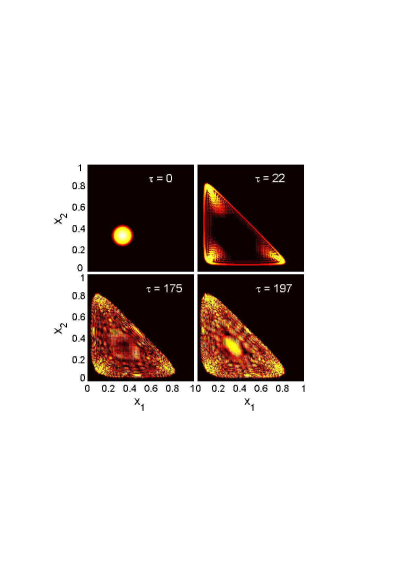
Figure 1: Quantum evolution of $N=200$ BEC atoms loaded into the high symmetry points $X_{1}$, $X_{2}$ and $X_{3}$. The lattice constant is $\Lambda=0.21$. We use the initial state as in Eq.(37) with $\sigma=\sqrt{N/2}$ with the initial populations $(x_{1},x_{2})=(0.330,0.337)$ and phases $(\phi_{1},\phi_{2})=(0.02,-0.02)$. The initial stage of evolution is given in the upper two panels, while the lower two panels show an oscillating state by which the initial (localized) state is replaced.

The emergent state can be approximated by a linear combination of a small number of the phase states. The one-dimensional phase states are defined here via the discrete Fourier transform (DFT)

$$|\theta_{\ell}\rangle=\frac{1}{\sqrt{N+1}}\sum_{n=0}^{N}e^{in\theta_{\ell}}|n\rangle,$$ (40)

where $\theta_{\ell}=\frac{2\pi\ell}{N+1}$. Evidently $\langle\theta_{\ell^{\prime}}|\theta_{\ell}\rangle=\delta_{\ell^{\prime},\ell}$. Therefore, the phase states give another basis of the Hilbert space, in fact

$$|n\rangle=\frac{1}{\sqrt{N+1}}\sum_{\ell=0}^{N}e^{-in\theta_{\ell}}|\theta_{\ell}\rangle.$$ (41)

For a fixed total number of atoms $n_{1}+n_{2}+n_{3}=N$ the three-dimensional phase states are projected onto a two-dimensional subspace, i.e. the wave function can be written as

$$|\Psi\rangle=\sum_{\ell_{1}=0}^{N}\sum_{\ell_{2}=0}^{N}\hat{C}_{\ell_{1},\ell_{2}}|\theta_{\ell_{1}},\theta_{\ell_{2}}\rangle,$$ (42)

where

$$\hat{C}_{\ell_{1},\ell_{2}}\equiv\frac{1}{N+1}\sum_{k_{1}=0}^{N}\sum_{k_{2}=0}^{N-k_{1}}e^{-ik_{1}\theta_{\ell_{1}}-ik_{2}\theta_{\ell_{2}}}C_{k_{1},k_{2}}$$ (43)

is nothing but the DFT of the coefficients $C_{k_{1},k_{2}}$ extended over whole domain of $0\leq k_{1,2}\leq N$ by padding them with zeros. Note that the phase $\theta$ is half of the value of the semi-classical phase $\phi$ in the limit $h\to 0$.

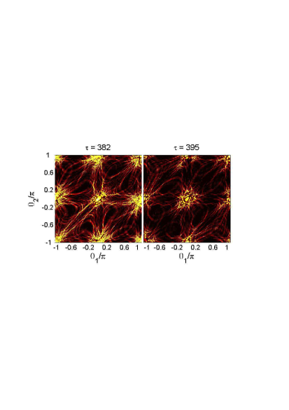
Figure 2: The DFT transform of the wave function of Fig. 1 at two large times (two panels are used to show the relatively small deformation with time).

We find that the DFT of the wave function of Fig. 1 is concentrated at the following values of the phases $\theta_{\ell}=\{0,\pm\pi\}$, see Fig. 2. These states correspond to the phases $\phi_{j}=0$ in the semi-classical limit, i.e. to the phases of the stationary point $P_{1}$.

The quantum evolution of the initial state corresponding to a stable classical stationary point as $h\to 0$ is different, see Fig. 3. First of all, the localized (i.e. nearly Fock) state remains localized. Note that the quantum and the semi-classical dynamics are very close in this case, see Fig. 4, though the number of atoms is rather small.

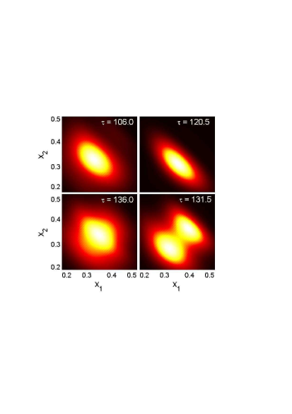
Figure 3: Quantum evolution of an initial Gaussian state of $N=200$ BEC atoms with $\sigma=\sqrt{N}$, the initial populations $(x_{1},x_{2})=(0.35,0.32)$, and phases $(\phi_{1},\phi_{2})=(0.01,-0.02)$. The lattice constant $\Lambda=0.36$, i.e. the semi-classical state $P_{1}$ is stable. Oscillations of the wave function about the initial state are observed (the time increases clock-wise).

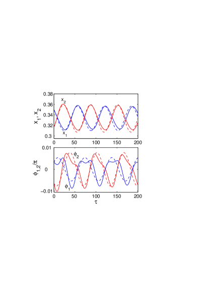
Figure 4: Comparison of the quantum evolution of Fig. 3 with the semi-classical evolution corresponding to the initial average values of the populations and phases. The upper and lower panels show average populations and phases, respectively.

In the nonlinear tunneling of BEC in a square 2D optical lattice SK (where the two-mode model appears) the quantum evolution features appear as collapses and revivals of the semi-classical dynamics. The energy spacing $\delta E\sim N^{-2}$ discussed in in Sec. II for the three-mode model (as compared to $\delta E\sim N^{-1}$ for the two-mode model) prevents observation of the quantum collapse. Indeed, the semi-classical regime requires large number of atoms, thus large evolution times $\tau\sim N^{2}$ are required for observation of the first quantum collapse. We verified that the quantum oscillations of Fig. 4 follow the semi-classical ones without occurrence of the quantum collapse for times up to $\tau=60000$ at least, which would exceed by far the lifetime of BEC (see Sec. II). This result also suggests that the quantum collapse may not exist in the model at all.

IV.3 Quantum evolution about the $P_{2}$-state

The above results show that the quantum model of $N$ identical bosons distinguishes between the stable and unstable classical stationary points. This conclusion agrees with the correspondence between the quantum stability of a semi-classical state in a system of identical bosons and the Hamiltonian stability of the corresponding stationary point in the classical limit QStab .

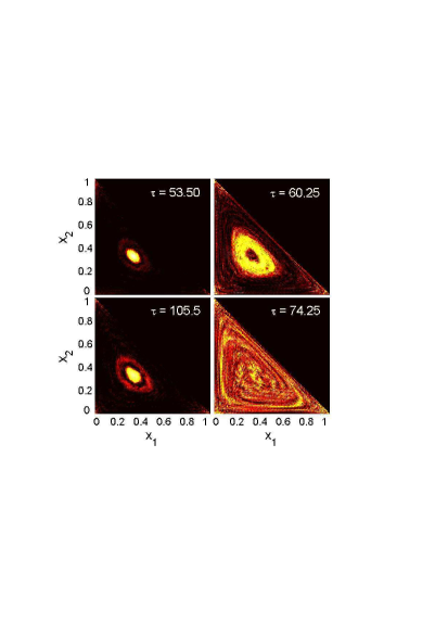
Figure 5: Recurrence of the wave function in quantum evolution (the time increases clock-wise) of an initial Gaussian state of $N=200$ BEC atoms with $\sigma=\sqrt{N}$, the initial populations $(x_{1},x_{2})=(0.330,0.337)$, and phases $(\phi_{1},\phi_{2})=\pi(2/3+0.01,-2/3+0.006)$. The lattice constant $\Lambda=0.64$, i.e. the semi-classical state $P_{2}$ is stable.

However, due the discreteness of the quantum energy levels the quantum evolution can have features not found in the classical model (the two cases, of course, agree in the limit $N\to\infty$ when the quantum energy spacing goes to zero). This is clearly illustrated by the results presented in Figs. 5 and 6. Indeed, Fig. 5 illustrates one period of the wave-function spread and subsequent recurrence to the localized distribution, which is responsible for the deviation of the quantum averages from the corresponding classical variables, see Fig. 6. Note however, that the quantum averages remain close to the the classical stationary point values, in accordance with the general correspondence of the quantum and classical stability QStab .

Figure 6: Comparison of the quantum evolution of Fig. 5 (solid lines) with the semi-classical result corresponding to the initial average values of the populations and phases. The upper panel gives the average populations and the lower one the phases (dashed lines). Top panel gives the population $x_{1}$ and the bottom one the phase $\phi_{1}$.

One more difference is apparent in Fig. 6 as compared with Fig. 4: the semi-classical dynamics about the $P_{2}$-point features two frequencies instead of one, as it is for the $P_{1}$-point. Despite the disagreement of the quantum averages and the classical dynamics, the recurrence period is in fact very close to one of the classical oscillations periods $\tau\sim 50$.

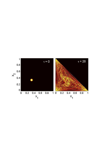
Figure 7: Quantum evolution of an initial Gaussian state of $N=200$ BEC atoms with $\sigma=\sqrt{15}$, the initial populations $(x_{1},x_{2})=(0.3300.337)$, and phases $(\phi_{1},\phi_{2})=\pi(2/3+0.07,-2/3+0.07)$. The lattice constant $\Lambda=0.69$ and the semi-classical state $P_{2}$ is unstable.

The quantum dynamics corresponding to the unstable classical fixed point $P_{2}$ is similar to that in the case of unstable $P_{1}$-point, namely the localized, i.e. nearly Fock-state, is replaced by a linear combination of a small fraction of the phase states, see Figs. 7 and 8. The phase states of Fig. 8 are concentrated about the following phases:

$$\biggl{\{}\left(-\frac{2\pi}{3},-\frac{\pi}{3}\right),\left(-\frac{2\pi}{3},\frac{2\pi}{3}\right),\left(-\frac{\pi}{3},\frac{\pi}{3}\right),\left(\frac{\pi}{3},\frac{2\pi}{3}\right),$$

$$\left(-\frac{\pi}{3},-\frac{2\pi}{3}\right),\left(\frac{2\pi}{3},-\frac{2\pi}{3}\right),\left(\frac{\pi}{3},-\frac{\pi}{3}\right),\left(\frac{2\pi}{3},\frac{\pi}{3}\right)\biggr{\}},$$

which correspond to the classical phases $(\phi_{1},\phi_{2})=\left\{\left(\pm\frac{2\pi}{3},\mp\frac{2\pi}{3}\right)\right\}$, i.e. to the phases of the stationary point $P_{2}$ and its equivalent $P^{\prime}_{2}$.

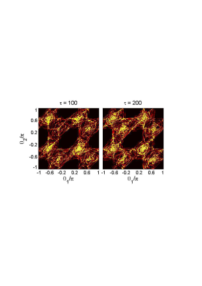
Figure 8: The DFT transform of the wave function represented in the right panel of Fig. 7.

For a special initial atomic distributions it is possible to have stable-like quantum dynamics about an unstable semi-classical fixed point which is conditionally stable for the special initial conditions. For instance, the fixed point $P_{3}$ is stable for the initial states with no $(p_{2},q_{2})$-components in the classical limit (which is supposed to be a small perturbation about the fixed point). In this case the wave function remains localized and performs oscillations about the initial state (not shown).

As the stationary points corresponding to unequal populations of the $X$-points of the lattice are unstable and loading BEC into the unequal distribution among the high-symmetry points is not an easy (if at all possible) task we discard the further analysis of the dynamics about the points $P_{3}$, $P_{4}$ and $P^{\prime}_{4}$.

IV.4 Dynamics of the boundary states

One can easily load BEC into a single $X$-point by switching on a moving cubic lattice. Thus, it is important to consider the boundary stationary point $P_{B_{1}}$. Let us consider X₃-point being initially populated. For $\Lambda<1/3$ the point $P_{B_{1}}$ is classically stable and the quantum dynamics consists of localized oscillations about the initial state. If however, the lattice parameter passes the critical value $\Lambda_{1}$ the instability of $P_{B_{1}}$ results in tunneling to the equal distribution of atoms between the three X-points, see Fig. 9.

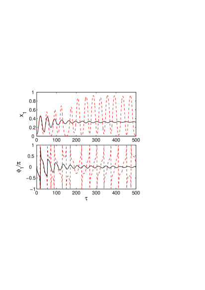
Figure 9: Comparison of the quantum evolution (solid lines) of with the semi-classical one (dashed lines). The upper panel gives the average population $x_{1}$ and the lower one the phase $\phi_{1}$. Here the initial populations and phases are $(x_{1},x_{2})=(0.04,0.04)$ and $(\phi_{1},\phi_{2})=(0.05,0)$, the lattice parameter $\Lambda=0.41$, $N=200$, and $\sigma=\sqrt{N}$. The stationary point $P_{B_{1}}$ ($x_{3}=1$) is unstable.

The dynamical instability of the $P_{B_{1}}$ can be used to prepare the system in the equal distribution of atoms between the $X$-points by loading first the $P_{B_{1}}$-point as discussed above and modifying the lattice parameter $\Lambda$ to force the dynamical instability of $P_{B_{1}}$ to develop, i.e. as shown in Fig. 9. The oscillations in Fig. 9 are about an equal distribution of atoms between the $X$-points and the zero phases, thus the quantum state is the semiclassical state about the $P_{1}$-point of the form given by equation (37) (or a linear combination of such states). Moreover, one can notice that the energy of a stationary semiclassical state ($N\gg 1$) in the main order is given by the zero-point energy of the local classical Hamiltonian, since the energy spacing between the local bound states is on the order or smaller than $1/N$ (since the quantum oscillator model, obtained by the “reverse quantization” procedure of the local classical Hamiltonian, has the energy spacing $O(h)$). Comparing the energies $E_{P_{2},P_{2}^{\prime}}=\Lambda/2-1/3+O(1/N)$ and $E_{P_{1}}=-1/3+O(1/N)$, we see that the ground state for $\Lambda\geq 1/3$ corresponds to the $P_{1}$-point.

On the other hand, the $P_{2}$-point and its equivalent point $P_{2}^{\prime}$ are stable and $P_{1}$ is unstable for $\Lambda<1/3$ (see table 1). Note also that the zero-point energy of $E_{P_{2}}=\Lambda/2<1/6$ is lower than that of $E_{P_{B_{1}}}=1/4$, another stable point for $\Lambda<1/3$. Thus, given the quantum state with an equal distribution between the $X$-points, i.e. $P_{1}$, one can prepare another such stable state (in fact $P_{2}$ or $P_{2}^{\prime}$ or their linear combination) by repeating the above procedure but now starting from the $P_{1}$-point by adiabatically changing the lattice parameter to $\Lambda<1/3$ followed by the thermal cooling procedure.

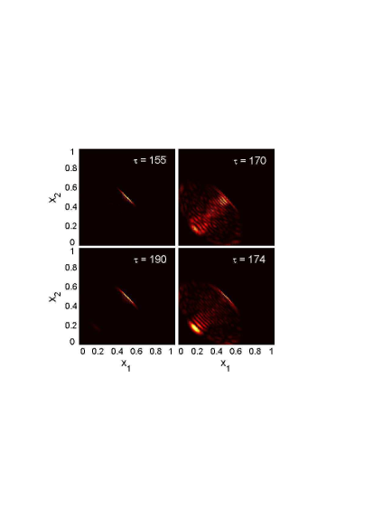
Figure 10: Quantum evolution of a state corresponding to initially almost equally populated two X-points (here X₁ and X₂). The time increases clock-wise. Here the initial populations and phases are $(x_{1},x_{2})=(0.48,0.48)$ and $(\phi_{1},\phi_{2})=\phi_{\Lambda}(0.98,1.03)$, the lattice parameter $\Lambda=0.51$, $N=200$, and $\sigma=\sqrt{N}$.

Stationary point $P_{B_{2}}$ is unstable in the domain of its existence $\Lambda\geq 1/3$ (except for the critical value $\Lambda=1/3$). This stationary point corresponds to the quasi 2D stationary state, however its instability rules out observation of 2D quantum dynamics SK , for instance the quantum collapses and revivals. We have found that an initial state with almost equal distribution of atoms between two $X$-points results in the sequence of quantum recurrences, when the wave function returns to a state with almost all atoms distributed among the initially populated points, see Fig. 10 (in the figure this state corresponds to an extended population on the line $x_{1}+x_{2}=1$).

V Discussion

The nonlinear tunneling of BEC with a large number of atoms $N$ can be considered in the semi-classical approximation, with the effective Planck constant being $h=1/N$. We have considered the correspondence between the semi-classical regime (equivalent to the mean-field regime) and the full quantum regime of nonlinear tunneling between the $X$-points of the Brillouin zone of a cubic 3D lattice. In particular, we have derived a quantum three-mode model and rewritten it as a two-dimensional Schrödinger equation for an effective quantum particle, where the effective Plank constant is $1/N$, the time scale is determined solely by the nonlinearity of BEC, while the dynamics is controlled by a lattice parameter $\Lambda$. The corresponding semi-classical model is the mean-field approach taking into account the occupations of the $X$-points only. Though we have used rather small number of atoms, $N=200$, we have found the regimes of excellent correspondence, these are mainly about the stable stationary points of the mean-field approach. In particular, numerical simulations show that the quantum dynamics about the semi-classical stationary point distinguishes the stable and unstable cases. In the case of a stable semi-classical point, one scenario consists of the wave function performing oscillations about the initial state with the averages following the semi-classical dynamics. The discreteness of the quantum energy space, however, leads to a scenario not present in the semi-classical case: the sequence consisting of the wave function spread (i.e. becoming a nearly phase-state) followed by the quantum recurrence to the initial nearly Fock state. This is reflected in a deviation of the quantum averages from the semi-classical dynamics. In the case of an unstable stationary point, the initially localized state, i.e. nearly Fock state, is replaced by a nearly phase state with the phases concentrated at the semi-classical value corresponding to the unstable point (more precisely, a linear combination of nearly phase states, since the quantum phase appearing in the wave function of the effective quantum particle is equal to half of the semi-classical phase due to the symmetry of the quantum Hamiltonian).

Existence of the stable stationary point with all atoms populating just one $X$-point of the lattice allows for the experimental study of the 3D nonlinear tunneling by modifying the optical lattice to change the value of the lattice parameter $\Lambda$. When the instability of the singly-populated $X$-point is reached by varying $\Lambda$, the quantum evolution quickly establishes equal distribution between the three degenerate $X$-points.

Appendix A The estimate (16)

We will use the inequality

$$|\langle(b^{\dagger}_{j})^{2}b^{2}_{k}+(b^{\dagger}_{k})^{2}b^{2}_{j}\rangle|\leq\langle n_{j}(n_{j}-1)+n_{k}(n_{k}-1)\rangle,$$ (44)

which follows from

$$0\leq\langle\Phi|(A+B)^{\dagger}(A+B)|\Phi\rangle$$

$$=\langle\Phi|A^{\dagger}A|\Phi\rangle+\langle\Phi|B^{\dagger}B|\Phi\rangle+\langle\Phi|A^{\dagger}B|\Phi\rangle+\langle\Phi|B^{\dagger}A|\Phi\rangle$$

by setting $A=b_{j}^{2}$ and $B=\pm b_{k}^{2}$. Using (44) we obtain

$$\langle\hat{H}_{-}\rangle\leq\langle\hat{H}\rangle\leq\langle\hat{H}_{+}\rangle,$$ (45)

where $\hat{H}_{\pm}$ are two $c$-number operators:

$$\hat{H}_{\pm}=\frac{1}{4}\sum_{j=1}^{3}\frac{n_{j}^{2}}{N^{2}}+\Lambda\sum_{j<k}\frac{n_{j}}{N}\frac{n_{k}}{N}\pm\frac{\Lambda}{2}\sum_{j=1}^{3}\frac{n_{j}}{N}\frac{n_{j}-1}{N},$$

which may be treated as classical functions of $n_{j}$. Next, reducing the total squares $(\sum_{j=1}^{3}n_{j}/N)^{2}=1$ in $\hat{H}_{\pm}$ we have

$$\hat{H}_{+}=\frac{1}{4}\sum_{j=1}^{3}\frac{n_{j}^{2}}{N^{2}}+\frac{\Lambda}{2}\left(1-\frac{1}{N}\right),$$ (46)

$$\hat{H}_{-}=\frac{1-4\Lambda}{4}\sum_{j=1}^{3}\frac{n_{j}^{2}}{N^{2}}+\frac{\Lambda}{2}\left(1+\frac{1}{N}\right).$$ (47)

The inequalities (16) follow from (46) and (47) if one takes into account that $N^{2}/3\leq\sum_{j=1}^{3}{n_{j}^{2}}\leq N^{2}$.

Appendix B The semi-classical stationary solutions with only two populated X-points

Consider the Hamiltonian (12) in the semi-classical limit, i.e. $b_{j}\to\sqrt{N}b^{(cl)}_{j}$. Suppose that there is a stationary point with $b_{10}=\cos\theta e^{-i\phi_{1}/2}$, $b_{20}=\sin\theta e^{-i\phi_{2}/2}$, and $b_{30}=0$ with some $0<\theta<\pi/2$. To find all such stationary points we use that the semi-classical Hamiltonian expanded about such a point does not have any linear terms. Without loss of generality we can set

$$b_{1} = \cos\theta e^{-i\phi_{1}/2}(1+\beta_{1}),\,b_{2}=\sin\theta e^{-i\phi_{1}/2}(1+\beta_{2}),$$

$$b_{3} = \beta_{3}\in\mathrm{Re}$$ (48)

where, due to the conservation of the number of atoms, in the linear order we get

$$\beta_{3}^{2}=-\cos^{2}\theta(\beta_{1}+\beta_{1}^{*})-\sin^{2}\theta(\beta_{2}+\beta_{2}^{*}).$$ (49)

Using this we obtain the linear in $\beta_{1,2}$ terms as follows:

$$\frac{\partial\mathcal{H}}{\partial\beta_{1}}\biggr{|}_{\beta_{1,2}=0}=\cos^{2}\theta\biggl{[}\frac{\cos^{2}\theta}{2}-\Lambda\cos^{2}\theta$$

$$+\frac{\Lambda}{2}\biggl{(}\sin^{2}\theta e^{i(\phi_{2}-\phi_{1})}-\cos^{2}\theta\cos\phi_{1}-\sin^{2}\theta\cos\phi_{2}\biggr{)}\biggr{]}.$$

(50)

In calculation of (50) we have used that the contributing terms are

$$\mathcal{H}_{\mathrm{\beta_{1}}} = \frac{1}{4}n_{1}^{4}+\Lambda[n_{1}n_{2}+n_{1}n_{3}+n_{2}n_{3}]$$

$$+ \frac{\Lambda}{4}[(b_{2}^{*})^{2}b_{1}^{2}+(b_{3}^{*})^{2}b_{1}^{2}+(b_{3}^{*})^{2}b_{2}^{2}+(b^{*}_{2})^{2}b_{3}^{2}].$$

By changing $\cos\theta\to\sin\theta$ and $\phi_{1}\to\phi_{2}$ we have also

$$\frac{\partial\mathcal{H}}{\partial\beta^{*}_{2}}\biggr{|}_{\beta_{1,2}=0}=\sin^{2}\theta\biggl{[}\frac{\sin^{2}\theta}{2}-\Lambda\sin^{2}\theta$$

$$+\frac{\Lambda}{2}\biggl{(}\cos^{2}\theta e^{i(\phi_{2}-\phi_{1})}-\sin^{2}\theta\cos\phi_{2}-\cos^{2}\theta\cos\phi_{1}\biggr{)}\biggr{]}.$$

(51)

The r.h.s.’s in equations (50), (51) and in their complex conjugates should give zero for a stationary solution. First of all, from (50) we have $\sin(\phi_{2}-\phi_{1})=0$, hence $\phi_{2}=\phi_{1}$ or $\phi_{2}=\phi_{1}\pm\pi$. Then, combining equations (50), (51) we get

$$(\cos^{2}\theta-\sin^{2}\theta)\left(\frac{1}{2}-\Lambda-\frac{\Lambda}{2}\cos(\phi_{2}-\phi_{1})\right)=0,$$

i.e. ($i$) $\cos\theta=\sin\theta=1/\sqrt{2}$ or ($ii$) $\cos(\phi_{2}-\phi_{1})=\frac{1-2\Lambda}{\Lambda}$. In case ($i$) we obtain the phase $\cos(\phi_{\Lambda})=\frac{1-\Lambda}{2\Lambda},$ while in case ($ii$) there is no solution except for the special value of the lattice parameter $\Lambda=1/3$ when the phase $\phi_{1}$ becomes arbitrary. Hence, we arrive at the stationary point $(x_{1},x_{2},x_{3})=\left(\frac{1}{2},\frac{1}{2},0\right)$, $\phi_{1}=\phi_{2}=\phi_{\Lambda},$ which exists only for $\Lambda\geq\Lambda_{1}=1/3$ (the phases appear in the initial state (37)). In terms of $z$-variables the stationary point reads $z_{1}=z_{2}=0$.

References

- (1) V. S. Shchesnovich and V. V. Konotop, Phys. Rev. A 75, 063628 (2007).
- (2) C. W. Gardiner, Phys. Rev. A 56, 1414 (1997);
- (3) V. A. Brazhnyi, V. V. Konotop, and V. Kuzmiak, Phys. Rev. Lett. 96 150402 (2006).
- (4) V. A. Brazhnyi, V. V. Konotop, V. Kuzmiak, and V. S. Shchesnovich, Phys. Rev. A 76, 023608 (2007).
- (5) A. Vardi and J. R. Anglin, Phys. Rev. Lett. 86, 568 (2001); J. R. Anglin and A. Vardi, Phys. Rev. A 64, 013605 (2001).
- (6) V. V. Konotop and P. G. Kevrekidis, Phys. Rev. Lett. 91, 230402 (2003).
- (7) C. A. Blockley, D. F. Walls, and H. Risken, Europhys. Lett, 17, 509 (1992) J. I. Cirac, R. Blatt, A. S. Parkins, and P. Zoller, Phys. Rev. A 49, 1202 (1994)
- (8) V. A. Brazhnyi and V. V. Konotop, Mod. Phys. Lett. B 18, 627 (2004).
- (9) O. Morsch and M. Oberthaler, Rev. Mod. Phys. 78, 179 (2006).
- (10) P. A. Braun, Rev. Mod. Phys. 65, 115 (1993).
- (11) H. Tal-Ezer and R. Kosloff, J. Chem. Phys. 81, 3967 (1984).
- (12) V. S. Shchesnovich, Phys. Lett. A, 349, 398 (2006).