Resource allocation pattern in infrastructure networks

Abstract

Most infrastructure networks evolve and operate in a decentralized fashion, which may adversely impact the allocation of resources across the system. Here we investigate this question by focusing on the relation between capacity and load in various such networks. We find that, due to network traffic fluctuations, real systems tend to have larger unoccupied portions of the capacities—smaller load-to-capacity ratios—on network elements with smaller capacities, which contrasts with key assumptions involved in previous studies. This finding suggests that infrastructure networks have evolved to minimize local failures but not necessarily large-scale failures that can be caused by the cascading spread of local damage.

Published in: J. Phys. A: Math. Theor. 41 (2008) 224019.

1 Introduction

Power outages, Internet congestion, traffic jams, and many other problems of social and economical interest are ultimately limited by the physical assignment of resources in infrastructure networks. The recent realization that numerous such systems can be modeled within the common framework of complex networks [1] has stimulated several theoretical studies on network resilience [2, 3, 4, 5, 6, 7, 8, 9, 10, 11, 12, 13, 14, 15, 16, 17, 18, 19, 20]. However, despite much advance [21], the relation between the large-scale allocation and actual usage of resources in distributed infrastructure systems is a question that goes beyond previous complex network research. Here we propose to cast this question as a statistical physics problem by exploring that the dynamics of many such systems can be modeled as a network transport process. For example, website browsing and e-mail communication are based on packet transport through the Internet; movement of people and goods is heavily based on road, rail, and air transportation networks; public utility services depend on the transport of energy, water and gas through supply networks. In these examples, the transport of packets, passengers, and physical quantities creates traffic loads that must be handled by nodes and links of the underlying networks. Because the capacities of nodes and links are limited by cost and availability of resources, the proper allocation of capacities is an essential condition for the robust and cost-effective operation of infrastructure networks.

In this paper, we investigate this question by focusing on the relationship between capacity and load from the perspective of a decentralized optimization between robustness and cost. By analyzing four types of infrastructure networks, the air transportation, highway, power-grid and Internet router network, we find empirically that the capacity–load relation is mainly determined by the relative importance given to the cost: if robustness is much more important than cost, the capacity $C$ approaches the line of maximum robustness $C=C_{\max}$, where $C_{\max}$ is the maximum available capacity, irrespective of the load; if cost is a strongly limiting factor, the capacity approaches the line of maximum efficiency $C=L$, for all values of the load $L$. The real systems analyzed fall in between these two extremes and exhibit an unanticipated nonlinear behavior, which, as shown schematically in Figure 1, is very different from the constant [11, 13], random [14, 15], and linear [16, 17, 18, 19] assignments of capacities considered in previous models. We study this nonlinearity using the concept of unoccupied capacity, the difference between the capacity and the time-averaged load. It follows, surprisingly, that the percentage of unoccupied capacity is smaller for network elements with larger capacities. Interpreting this as a result of a decentralized evolution in which capacities and loads are allocated or reallocated in response to increasing load demand [22], we demonstrate the observed behavior using a traffic model devised to minimize the probability of overloads in a scenario of fluctuating traffic and limited availability of resources. Our model shows that the reduction of the unoccupied capacity is a consequence of the reduction of the traffic fluctuations on highly loaded elements, but it also shows that the probability of overloads can be larger on elements with larger capacities.

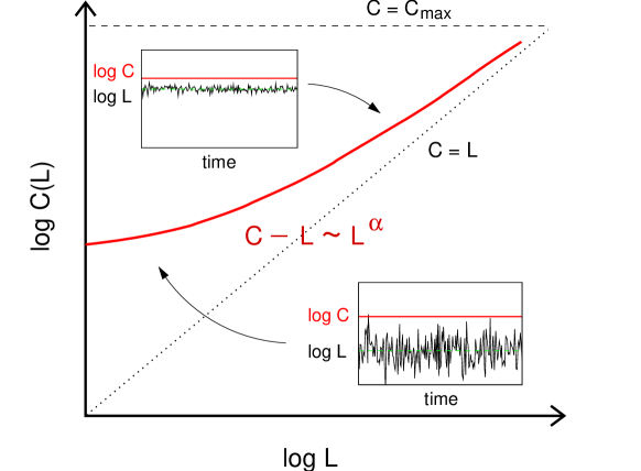
Figure 1: Typical capacity–load relation observed in real infrastructure networks. The nonlinear behavior of the capacity contrasts with the linear models $C\propto L$ hypothesized in previous network-theoretical work. Insets indicate traffic fluctuations as the expected origin of the observed nonlinearity.

2 Empirical Capacity-Load Characteristics

We consider four different types of real-world infrastructure networks: air transportation network, using seat occupation data of aircraft operating between $1449$ US and foreign airports available at the Bureau of Transportation Statistics database (http://www.bts.gov); highway network, using traffic data of the state of Colorado for $1559$ highway segments available at the Colorado Department of Transportation database (http://www.dot.state.co.us); power-grid network, using available data for $5885$ transmission lines of the Electric Reliability Council of Texas (http://www.ercot.com); Internet router network, using packet traffic data measured by the Multi Router Traffic Grapher (http://oss.oetiker.ch/mrtg/) on $721$ routers of the ABILENE backbone, MIT and Princeton University.

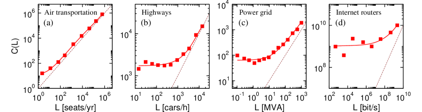
Figure 2: Capacity–load relation of four real networks. (a) Total number of occupied ($L$) versus available seats ($C$) in aircraft departing from and arriving at US and international airports in $2005$. (b) Design hourly volume ($L$) versus estimated capacity ($C$) of Colorado highway segments in $2005$. (c) Apparent power ($L$) versus corresponding capacity ($C$) of transmission lines in the power grid of Texas at the summer peak in $2000$. (d) Monthly averaged traffic ($L$) versus bandwidth ($C$) of the router interfaces of the ABILENE backbone, MIT and Princeton University networks in June $2006$. The filled boxes with curve fits indicate the averaged capacity–load relation $C(L)$ calculated in a logarithmic scale. The line of maximum efficiency $C=L$ (dashed line) is shown for comparison with the real data.

Figure 2 shows the relation between the time-averaged load and capacity of the network elements in a log-binned scale. The air transportation network [Figure 2(a)] is very close to the line of maximum efficiency $C=L$, indicating effective allocation of resources, which is likely to be a consequence of the high costs of air transportation combined with flexibility to adjust seat availability to demand. The highway network shows less efficient behavior in the region of small loads [Figure 2(b)], a feature that may provide alternative routes for congested traffic. A similar pattern is observed in the power-grid network [Figure 2(c)] although, compared to the highway network, the power grid has larger unoccupied capacities for the heavily loaded components of the network. These unoccupied capacities can be useful for the dispatch of power generation to adjust to specific market, weather, and demand conditions. The Internet router network [Figure 2(d)] shows weaker dependence of the capacity on the load than those found in the other networks, which is probably due to the discreteness of the commercially available router bandwidths, the fast growing bandwidth demand, and the tendency to simultaneously upgrade groups of routers regardless of their individual loads. Therefore, while the capacity–load relation depends on the specific network, the pattern of this dependence can be understood in connection with a trade-off between the robustness and the cost of capacities in the construction and maintenance of the system.

For quantitative characterization, we define the efficiency coefficient $\varepsilon$ of a network as the ratio between the total load and total capacity,

$$\varepsilon=\frac{\sum_{i}L_{i}}{\sum_{i}C_{i}},$$ (1)

where the sums are taken over all components of the system. This quantity provides a measure of the importance of the cost. As the cost becomes more important, the capacity is expected to approach the load in order to prevent overallocation of resources, which increases $\varepsilon$; when the robustness is more important, the capacity is expected to be much larger than the load, which decreases $\varepsilon$. We find that the efficiency coefficient is $\varepsilon=0.73$ for the air transportation network, $0.54$ for the highway network, $0.29$ for the power-grid network, and $0.06$ for the Internet router network. Therefore, one can argue that cost is increasingly deprioritized over robustness as one goes from the air transportation to the highway, power-grid and Internet router network. In particular, the average unused capacity reaches $94\%$ in the Internet router network as opposed to $27\%$ in the air transportation system.

In interpreting these results one should notice that the capacities of the air transportation network can be easily downgraded while the same does not hold true for the other networks. Power transmission lines, highways, and Internet hardware involve permanent allocation of physical capacities that cannot be dynamically adjusted or redistributed across the system. The presence of network elements (nodes and links) with finite minimum physical capacities is likely to be a contributing factor for the plateaus observed in the region of small loads [Figure 2(b)-(d)].

3 Capacity Optimization Model

We now analyze our empirical findings using a model based on the optimization of capacities at the level of individual network elements. We define a simple objective function $F_{i}=(1-w)R_{i}(C_{i})+wS_{i}(C_{i})$ for node $i$, which incorporates competing robustness ($R_{i}$) and cost $(S_{i})$ functions, and where $w\in[0,1]$ represents the importance of the cost. Given functions $R_{i}$ and $S_{i}$, the minimization of $F_{i}$ will lead to an optimized capacity $C_{i}$ for node $i$ subjected to the time-averaged load $L_{i}$, which defines a capacity–load relation $C(L)$. To formulate this model, we consider a time-dependent transport process in which traffic moves from source to destination along predetermined paths. This process includes as a special case the directed flow model where traffic moves along the shortest paths [24], and it leads to a general yet mathematically treatable model that is not dependent on the details of the network structure and routing scheme.

Within this model, we identify the time fluctuation of traffic as the main perturbation that can cause accidental overloading failures. Defining the robustness function $R_{i}$ as the overloading probability $\xi_{i}$, the objective function can be written as

$$F_{i}=(1-w)\xi_{i}(C_{i})+w\frac{C_{i}}{C_{\max}},$$ (2)

where, for concreteness, we have chosen the cost $S_{i}$ to be a linear function of the capacity.

To determine the overloading probability, we calculate the load $l_{i}(t)=\sum_{j,k}z_{jk;i}x_{jk;i}(t)$ on node $i$ at time $t$, where $x_{jk;i}(t)$ is the amount of the traffic towards node $k$ originating from node $j$ at time $t-\tau_{jk;i}$. Here, $z_{jk;i}$ is $1$ if $i$ lies on the path from $j$ to $k$ and $0$ otherwise. If we take a time window $\Delta t$ much larger than the autocorrelation time of $x_{jk;i}$’s, we can rewrite the time-averaged load $L_{i}$ as

$$L_{i}=\frac{1}{\Delta t}\int_{t}^{t+\Delta t}l_{i}(t^{\prime})dt^{\prime}\simeq\sum_{j,k}z_{jk;i}\langle x_{jk;i}\rangle,$$ (3)

where $\langle\cdot\rangle$ is used for ensemble averages. Then, given the distribution of $x_{jk;i}$, and thereby the load distribution $P_{i}(l_{i})$, we can write the overloading probability $\xi_{i}$ as

$$\xi_{i}(C_{i})=\textrm{Prob}[l_{i}>C_{i}]=\int^{\infty}_{C_{i}}P_{i}(l_{i})dl_{i}$$ (4)

for given capacity $C_{i}$ such that $L_{i}\leq C_{i}\leq C_{\max}$. The capacity $C$ is assumed to be physically upper-bounded by $C_{\max}$ and lower-bounded by $L$.

For the explicit calculation of the capacity–load relation, we consider uncorrelated and synchronized traffic fluctuations. We consider both types of fluctuations since random internal fluctuations can be strongly modulated by external driving forces [25]. In the Internet backbone, for example, it has been observed that the traffic dynamics is well-characterized by a Poisson process for millisecond time scales, while long-range correlations appear for longer time scales [26]. In the systems we consider, synchronized fluctuations can be generally triggered by exogenous factors, such as weather and seasonal conditions or collective human behavior.

Uncorrelated Fluctuations. We consider fluctuations in which the traffic $x_{jk;i}$ is completely uncorrelated with the traffic between different source-destination nodes. In this regime, the quantity $x_{jk;i}$ can be regarded as an independent identically distributed random variable $r$ following a probability distribution $p(r)$. Assuming that $p(r)$ has finite moments, including average $\bar{r}$ and variance $s^{2}$, we apply the central limit theorem to obtain a Gaussian distribution of loads,

$$P_{i}(l_{i})\simeq\frac{1}{\sigma_{i}\sqrt{2\pi}}\exp\left[-\frac{(l_{i}-L_{i})^{2}}{2\sigma_{i}^{2}}\right],$$ (5)

with average $L_{i}=\bar{r}\sum_{j,k}z_{jk;i}\equiv\bar{r}z_{i}$ and variance $\sigma_{i}^{2}=s^{2}z_{i}$. The relation $\sigma_{i}\sim L_{i}^{1/2}$, a corollary of Eq. (5), is in agreement with the empirical results of previous studies [24, 25, 27]. Now, using Eq. (5) in the minimization of $F_{i}$ in Eq. (2), we obtain the capacity–load relation as $C(L)=\min\{C^{\prime}(L),C_{\max}\}$ with

$$C^{\prime}(L)=\left\{\begin{array}[]{ll}L+gL^{\frac{1}{2}}\sqrt{\log\Omega(L)}&\textrm{if $L<L_{w}$}\\ L&\textrm{if $L>L_{w}$},\end{array}\right.$$ (6)

where $\Omega(L)\equiv\frac{1}{g\sqrt{\pi}}\frac{1-w}{w}\frac{C_{\max}}{L^{1/2}}$, parameter $g$ denotes $\sqrt{2s^{2}/\bar{r}}$, and $L_{w}$ satisfies $\Omega(L_{w})=1$.

Synchronized Fluctuations. Since the modulation of traffic that we describe by synchronized fluctuations occurs in a longer time scale [25, 27], we neglect the travel time $\tau_{jk;i}$ to express $x_{jk;i}(t)\equiv x(t)$ and the synchronized traffic load as $l_{i}(t)=x(t)z_{i}$. Assuming statistical independence of $x(t)$ in different modulation periods, we use the peak value $r$ of $x(t)$ in each modulation period as a reference for capacity determination. Given the distribution $p(r)$, we can write the overloading probability $\xi_{i}$ as

$$\xi_{i}(C_{i})=\int^{\infty}_{C_{i}}P(l_{i})dl_{i}=\int^{\infty}_{\bar{r}C_{i}/L_{i}}p(r)dr,$$ (7)

and determine $C(L)$ by minimizing $F_{i}$. The resulting optimized capacity is $C(L)=\min\{C^{\prime}(L),C_{\max}\}$, with

$$C^{\prime}(L)=\left\{\begin{array}[]{ll}\frac{L}{\bar{r}}\ q\big{(}\frac{w}{1-w}\frac{L}{\bar{r}C_{\max}}\big{)}&\textrm{if $L<L_{w}$}\\ L&\textrm{if $L>L_{w}$},\end{array}\right.$$ (8)

where $L_{w}=\bar{r}C_{\max}\frac{1-w}{w}\max_{r}p(r)$ and $q(y)=r$ is obtained by inverting $y=p(r)$. For $y=p(r)$ having more than one solution, we conventionally select $q(y)$ that gives the largest capacity. Because we have defined $r$ as the maximum traffic amount of many individual traffic events in a modulation period, extreme value distributions can be used as an input for $p(r)$. Here we numerically calculate $C(L)$ for the Gumbel distribution $p_{g}(r)=\frac{1}{\beta}\exp[-\frac{r-\mu}{\beta}-e^{-\frac{r-\mu}{\beta}}]$ and the Fréchet distribution $p_{f}(r)=\frac{\gamma}{\alpha^{-\gamma}}r^{-\gamma-1}\exp[-\big{(}\frac{r}{\alpha}\big{)}^{-\gamma}]$, where all parameters are positive, referred to as the first and second asymptotes in the extreme value statistics literature [28]. These two asymptotes correspond to exponential and power-law initial distributions, respectively. The third asymptote is for bounded initial distributions and gives similar results when the bound of the traffic $x(t)$ becomes large.

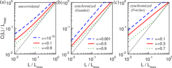
Figure 3: Capacity–load relation derived from the capacity optimization model for three values of the weight $w$ assigned to the cost: (a) uncorrelated fluctuation regime for the model parameter $g=3$; (b) synchronized fluctuation regime for the Gumbel distribution with parameters $(\mu,\beta)=(100,20)$; (c) synchronized fluctuation regime for the Fréchet distribution with parameters $(\alpha,\gamma)=(1,2)$. The capacity and load are normalized by the predefined maximum value $C_{\max}=L_{\max}=10^{3}$.

Figure 3 shows our model predictions for uncorrelated and synchronized fluctuations. In both regimes we find that the allocation of capacities exhibits characteristics in common with the empirical data. In particular, the calculated $C(L)$ shows the common trend that a larger relative deviation from the line $C=L$, representing a larger unoccupied portion of the capacity, is found in the region of smaller $L$. These results are determined by general statistical properties of the traffic and do not depend on the details of the network structure and dynamics. This generality represents an advantage over previous models based on betweenness centrality because the latter is only weakly correlated with the actual flows in the networks and cannot be used to predict $C(L)$. Note that betweenness centrality only accounts for the shortest paths, while $l_{i}$ in Eq. (3) accounts both for paths that are not necessarily the shortest and for non-uniform distributions of the “size” $x_{jk;i}$ of the individual traffic events.

4 Discussion

The observed nonlinearity in the capacity–load relation suggests that infrastructure systems have evolved under the pressure to minimize local failures rather than global failures. Previous work [20] has established that the incidence of large cascading failures can be reduced by shedding loads on low-load nodes, despite the fact that this causes a concurrent increase in the incidence of small failures. In the present model this would correspond to a higher probability of overloads for network elements subjected to smaller loads, which is the opposite of the trend observed in this study. Indeed, as a result of the optimization of capacities, the overloading probability $\xi(L)$ is an increasing function of $L$ and differs, in particular, from capacity allocations that assume the same overloading probability for all the nodes. The predicted vulnerability to large-scale failures is consistent with the absence of global optimization given that real infrastructure networks evolve in a decentralized way. In the case of the power grid, for example, it has been proposed [22] that the evolution of the system is driven by the opposing forces of slow load increase and corresponding system upgrades, keeping the system in a dynamic equilibrium that balances the probability of outages. It is likely that a similar self-organization mechanism is at work in infrastructure systems in general, which would further expand the concept of network self-organization [29] within transportation problems. While providing additional rationale for the decentralized optimization incorporated in our model, this view emphasizes that in infrastructure systems local robustness is prioritized at the expense of global robustness. These results are expected to enable researchers to build models to study network evolution and the impact of disturbances in complex communication and transportation systems.

References

References

- [1] Newman MEJ, Barabási A-L and Watts DJ (eds) 2006 The Structure and Dynamics of Networks (Princeton: Princeton University Press)
- [2] Albert R, Jeong H and Barabási A-L 2000 Nature 406 378–82
- [3] Callaway DS, Newman MEJ, Strogatz SH and Watts DJ 2000 Phys. Rev. Lett.85 5468–71
- [4] Cohen R, Erez K, ben-Avraham D and Havlin S 2000 Phys. Rev. Lett.85 4626–9
- [5] Shargel B, Sayama H, Epstein IR and Bar-Yam Y 2003 Phys. Rev. Lett.90 068701
- [6] Gallos LK, Cohen R, Argyrkis R, Bunde A and Havlin S 2005 Phys. Rev. Lett.94 188701
- [7] Arenas A, Díaz-Guilera A and Guimerà R 2001 Phys. Rev. Lett.86 3196–9
- [8] Toroczkai Z and Bassler KE 2004 Nature 428 716
- [9] Noh JD, Shim GM and Lee H 2005 Phys. Rev. Lett.94 198701
- [10] Sreenivasan S, Cohen R, López E, Toroczkai Z and Stanley HE 2007 Phys. Rev.E 75 036105
- [11] Holme P and Kim BJ 2002 Phys. Rev.E 65 066109
- [12] Motter AE, Nishikawa T and Lai Y-C 2002 Phys. Rev.E 66 065103
- [13] Moreno Y, Pastor-Satorras R, Vázquez A and Vespignani A 2003 Europhys. Lett. 62 292–8
- [14] Watts DJ 2002 Proc. Natl. Acad. Sci. USA 99 5766–71
- [15] Kim D-H, Kim BJ and Jeong H 2005 Phys. Rev. Lett.94 025501
- [16] Motter AE and Lai Y-C 2002 Phys. Rev.E 66 065103
- [17] Crucitti P, Latora V and Marchiori M 2004 Phys. Rev.E 69 045104
- [18] Lee EJ, Goh K-I, Kahng B and Kim D 2005 Phys. Rev.E 71 056108
- [19] Schäfer M, Scholz J and Greiner M 2006 Phys. Rev. Lett.96 108701
- [20] Motter AE 2004 Phys. Rev. Lett.93 098701
- [21] Barrat A, Barthélemy M, Pastor-Satorras R and Vespignani A 2004 Proc. Natl. Acad. Sci. USA 101 3747–52; Guimerà R, Mossa S, Turtschi A and Amaral LAN 2005 ibid. 102 7794–9
- [22] Dobson I, Carreras BA, Lynch VE and Newman DE 2007 Chaos 17 026103
- [23] Roughgarden T 2004 Selfish Routing and the Price of Anarchy (Cambridge: The MIT Press)
- [24] Arollo de Menezes M and Barabási A-L 2004 Phys. Rev. Lett.92 028701
- [25] Arollo de Menezes M and Barabási A-L 2004 Phys. Rev. Lett.93 068701
- [26] Karagiannis T, Molle M and Faloutsos M 2004 IEEE Internet Computing 8 57–64
- [27] Duch J and Arenas A 2006 Phys. Rev. Lett.96 218702
- [28] Gumbel EJ 1958 Statistics of Extremes (New York: Columbia University Press)
- [29] Garlaschelli D, Cappocci A and Caldarelli G 2007 Nat. Phys. 3 813–817