Theoretical aspects of quantum state transfer, correlation measurement and electron-nuclei coupled dynamics in quantum dots

Abstract

Photons and electrons are the key quantum media for the quantum information processing based on solid state devices. The essential ingredients to accomplish the quantum repeater were investigated and their underlying physics were revealed. The relevant elementary processes of the quantum state transfer between a single photon and a single electron were analyzed, to clarify the conditions to be satisfied to achieve the high fidelity of the quantum state transfer. An optical method based on the Faraday rotation was proposed to carry out the Bell measurement of two electrons which is a key operation in the entanglement swapping for the quantum repeater and its feasibility was confirmed. Also investigated was the quantum dynamics in the electron-nuclei coupled spin system in quantum dots and a couple of new phenomena were predicted related to the correlations induced by the hyperfine interaction, namely, bunching and revival in the electron spin measurements. These findings will pave the way to accomplish the efficient and robust quantum repeater and nuclear spin quantum memory.

1 INTRODUCTION

Coherent manipulation of quantum states is a critical step toward many novel technological applications ranging from manipulation of qubits in quantum logic gates[1, 2, 3, 4, 5] to controlling the reaction pathways of molecules. In the field of the quantum state control by optical means, both Rabi oscillation and quantum interference play the central roles. The exciton Rabi splitting was observed in the luminescence spectrum of a single InGaAs quantum dot and the exciton Rabi oscillation was also observed in the spectroscopy of a single GaAs or InGaAs quantum dot [6, 7, 8, 9, 10, 11, 12]. The two-qubit CROT (controlled rotation) gate operation was demonstrated using two orthogonally polarized exciton states and a biexciton state in a GaAs quantum dot[13]. Unfortunately, however, the decoherence/dephasing times of excitons and biexcitons in these quantum dots are limited by the radiative lifetimes($\sim$ 1 ns) even at low temperatures. Thus a qubit with a longer decoherence time is desirable for the application to the quantum information processing. Electron spins in semiconductor quantum dots (QDs) are considered as one of the most promising candidates of the building blocks for quantum information processing[14, 15] due to their robustness against decoherence effects[16, 17]. In double QD systems, initialization and coherent manipulation of the electron spin have been realized, with coherence times extending to $1~{}\mu$s[18, 19].

Recently, a quantum media converter from a photon qubit to an electron spin qubit was proposed for quantum repeaters[20, 21]. Quantum information can take several different forms and it is preferable to be able to convert among different forms. One form is the photon polarization and another is the electron spin polarization. Photons are the most convenient medium for sharing quantum information between distant locations. However, it is necessary to realize a quantum repeater in order to send the information securely over a very long distance overcoming the photon loss. A quantum repeater requires two essential ingredients, namely, the quantum state transfer between a photon and an electron spin and the correlation (Bell) measurement between two electrons created by the quantum state transfer from two different photons. Additionally it is desirable to have a long-lived quantum memory based on the nuclear spins. For the quantum state transfer, a strained InGaAs/InP quantum dot was proposed as a preferable device based on the $g$-factor engineering[22]. In the actual operation, the photoexcited holes are to be quickly swept out of the quantum dot to project the photon polarization onto the electron spin polarization, preserving the quantum coherence. We have analyzed the performance of this operation and clarified the conditions to be satisfied to achieve a high value of the purity of the transferred quantum state or the fidelity of the quantum state transfer.

Another fundamental element for realizing the quantum repeater is the Bell (quantum correlation) measurement for the entanglement swapping. In our case this measurement is carried out for two electrons which are created by the quantum state transfer from two separate photons. Here we propose an optical method to do this Bell measurement based on the Faraday (in the transmission geometry) or Kerr (in the reflection geometry) rotation and estimate the feasibility.

The electron spin decoherence time reported so far for low temperatures is about a few microsecond and is not sufficiently long for the secure quantum information processing. Thus the nuclear spin quantum memory will be eventually required and the robust quantum state transfer should be realized between the electron spin and the nuclear spins in order to store and retrieve the quantum information. For that purpose, the fundamental features of dynamics in the electron-nuclei coupled system should be investigated. Here we reveal a sequence of back-actions between the electron spin and the nuclear spins through the quantum state measurements and predict a couple of new phenomena. These findings will open the way to realize the quantum state purification of nuclear spins, elongation of the electron spin decoherence time and the nuclear spin quantum memory.

2 QUANTUM STATE TRANSFER

In the quantum state transfer between the photon qubit and the electron qubit, the one-to-one correspondence should be established between the photon polarization and the electron spin polarization. In other words, the one-to-one correspondence between the Poincare sphere for a photon and the Bloch sphere for an electron spin should be realized as perfectly as possible. Since the photon energy is independent of the polarization direction, the electron energy should also be independent of the spin direction. This can be realized by the $g$-factor engineering[22]. The light-hole exciton is preferable than the heavy-hole exciton because of the characteristic optical selection rule and the possible Zeeman splitting in the in-plane magnetic field. In order to have the light-hole states as the ground hole states, the strained quantum well (QW) structure is necessary and can be realized in InGaAs/InP QW structures. In these strained QW structures the light-hole states are written as[23]

$$|\frac{3}{2}\frac{1}{2}\rangle=\sqrt{\frac{2}{3}}|10\rangle|\alpha\rangle+\sqrt{\frac{1}{3}}|11\rangle|\beta\rangle\;,$$ (1)

$$|\frac{3}{2}-\frac{1}{2}\rangle=\sqrt{\frac{1}{3}}|1-1\rangle|\alpha\rangle+\sqrt{\frac{2}{3}}|10\rangle|\beta\rangle\;,$$ (2)

where the usual angular momentum representation $|j,m\rangle$ is employed and $|10\rangle|\alpha\rangle$ indicates a $p_{z}$-like orbital with the up-spin, for example. Then the relevant Hamiltonian for the light-hole states under an in-plane magnetic field along the $x$ axis are represented by

$$-g_{\ell h}\mu_{B}BS_{x}=-\frac{2}{3}g_{\ell h}\mu_{B}B\left(\begin{array}[]{cc}0&1\\ 1&0\end{array}\right)\;,$$ (3)

where $g_{\ell h}$ is the g-factor of the light-hole and the eigenstates are given by

$$|\ell h_{1}\rangle=\frac{1}{\sqrt{2}}\left(|\frac{3}{2}\frac{1}{2}\rangle+|\frac{3}{2}-\frac{1}{2}\rangle\right)\;,\quad|\ell h_{2}\rangle=\frac{1}{\sqrt{2}}\left(|\frac{3}{2}\frac{1}{2}\rangle-|\frac{3}{2}-\frac{1}{2}\rangle\right)\;.$$ (4)

The selection rules of the optical transition can be derived by taking into account the conservation of the orbital angular momentum and the decomposition of the linear polarization into the circular polarization:

$$\hat{x}\cos\omega t=\frac{1}{2}(\hat{x}+i\hat{y})\cos\omega t+\frac{1}{2}(\hat{x}-i\hat{y})\cos\omega t\;,$$ (5)

$$\hat{y}\cos\omega t=\frac{1}{2i}(\hat{x}+i\hat{y})\cos\omega t-\frac{1}{2i}(\hat{x}-i\hat{y})\cos\omega t\;,$$ (6)

where $\hat{x}\;(\hat{y})$ denotes the unit vector in the $x\;(y)$-direction. Assuming $|\ell h_{1}\rangle$ to be the ground hole state (namely, $g_{\ell h}>0$), we have the optical selection rules:

$$|\ell h\rangle_{1}\longrightarrow\frac{1}{\sqrt{2}}(|c\uparrow\rangle-|c\downarrow\rangle)=-\;|e_{1}\rangle$$ (7)

for the $x-$polarized light and

$$|\ell h\rangle_{1}\longrightarrow\frac{-i}{\sqrt{2}}(|c\uparrow\rangle+|c\downarrow\rangle)=-i\;|e_{2}\rangle$$ (8)

for the $y-$polarized light, respectively, where $|c\uparrow(\downarrow)\rangle$ represents the conduction band electron state with the up (down) spin in the $z$ direction and $|e_{1}\rangle(|e_{2}\rangle)$ is the electron eigenstate with the spin aligned in the $-x\;(x)$ direction. The schematic energy levels are plotted in Fig. 1.

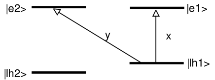
Figure 1: Schematic energy levels in a strained quantum well under an in-plane ($||x$) magnetic field.

According to these selection rules, we can excite a linear combination of exciton states which have a common hole state. When a linearly polarized light comes in with polarizaion given by

$$\cos\theta\;\hat{x}+\sin\theta\;\hat{y}\;,$$ (9)

the excited state can be written as

$$-\cos\theta|e_{1}\rangle|\ell h_{1}\rangle-i\sin\theta|e_{2}\rangle|\ell h_{1}\rangle=-\cos\theta|e_{1},h_{1}\rangle-i\sin\theta|e_{2},h_{1}\rangle\;,$$ (10)

where the direct product state $|e_{1}\rangle|\ell h_{1}\rangle$ is simply denoted by $|e_{1},h_{1}\rangle$ for example and the representation in the form of the electron-hole pair is used instead of the exciton representation. It is beyond the scope of this article to discuss fully the exciton effect in the quantum state transfer. Now we study influences of relaxation processes of the electron and the hole on the quantum state transfer. In the case of a gate-controlled quantum dot, the electron is three-dimensionally confined, whereas the hole is not confined and is absorbed into the negatively biased gate, leaving behind only the photoexcited electron. Thus the important issue is the quantum nature of the electron state after extraction of the hole: How much is the electron spin coherence retained after the process ? To answer this question, we will analyze the time evolution of the whole system based on the density matrix formalism. Just after the photoexcitation given by Eq. (10), the density matrix of the electron-hole system is supposed to be given by

$$\rho(t=0)=\cos^{2}\theta|e_{1},h_{1}\rangle\langle e_{1},h_{1}|+\sin^{2}\theta|e_{2},h_{1}\rangle\langle e_{2},h_{1}|$$

$$\hskip 36.98866pt+i\sin\theta\cos\theta|e_{2},h_{1}\rangle\langle e_{1},h_{1}|-i\sin\theta\cos\theta|e_{1},h_{1}\rangle\langle e_{2},h_{1}|\;.$$ (11)

Then the hole is extracted into the negatively biased gate electrode. In order to simulate this process, we introduce a model consisting of three hole states as depicted in Fig. 2; one of them is the hole state $|h_{1}\rangle$ created in a quantum dot by the photoexcitation, the second one is an intermediate hole state $|h_{2}\rangle$ representing a delocalized state around the gate electrode and the third one is the swept-out state in the gate. The most important mechanism degrading the electron spin coherence is the electron-hole exchange interaction which induces the spin state mixing. During the hole extraction to the negatively biased electrode the hole spin relaxation occurs and the electron spin states are mixed up, leading to the degradation of quantum state transfer.

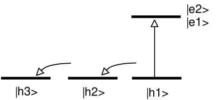
Figure 2: Schematic relaxation paths in the quantum state transfer from a photon to an electron spin. Curved arrows indicate the transfer (tunneling) process of the photoexcited hole. $|h3\rangle$ represents symbolically the final destination of the extracted hole.

2.1 Dynamics of quantum state transfer

To set up the equations of motion for the density matrix, we take into account six basis states composed of direct products of two electron states $|e_{1}\rangle$ and $|e_{2}\rangle$ and three hole states $|h_{1}\rangle\;,|h_{2}\rangle$ and $|h_{3}\rangle$:

$$|e_{1},h_{1}\rangle,|e_{2},h_{1}\rangle,|e_{1},h_{2}\rangle,|e_{2},h_{2}\rangle,|e_{1},h_{3}\rangle,|e_{2},h_{3}\rangle\;.$$ (12)

In this representation, the equation of motion for the density matrix is given by

$$\dot{\rho}=-\frac{i}{\hbar}[H,\rho]+\Gamma\rho\;,$$ (13)

$$H=H_{0}+H_{{\rm exch.}}\;,$$ (14)

$$H_{0}=E_{e}(|e_{1}\rangle\langle e_{1}|+|e_{2}\rangle\langle e_{2}|)-E_{h_{1}}|h_{1}\rangle\langle h_{1}|-E_{h_{2}}|h_{2}\rangle\langle h_{2}|-E_{h_{3}}|h_{3}\rangle\langle h_{3}|\;,$$ (15)

$$\Gamma\rho=t_{12}|h_{2}\rangle\langle h_{1}|\rho|h_{1}\rangle\langle h_{2}|+t_{23}|h_{3}\rangle\langle h_{2}|\rho|h_{2}\rangle\langle h_{3}|-t_{12}|h_{1}\rangle\langle h_{1}|\rho|h_{1}\rangle\langle h_{1}|$$

$$-t_{23}|h_{2}\rangle\langle h_{2}|\rho|h_{2}\rangle\langle h_{2}|-\sum_{i\neq j}\gamma^{h}_{ij}\{|h_{i}\rangle\langle h_{i}|\rho|h_{j}\rangle\langle h_{j}|+|h_{j}\rangle\langle h_{j}|\rho|h_{i}\rangle\langle h_{i}|\}$$

$$+\gamma^{e}_{1}|e_{2}\rangle\langle e_{1}|\rho|e_{1}\rangle\langle e_{2}|-\gamma^{e}_{1}|e_{1}\rangle\langle e_{1}|\rho|e_{1}\rangle\langle e_{1}|$$

$$-\gamma^{e}_{12}\{|e_{1}\rangle\langle e_{1}|\rho|e_{2}\rangle\langle e_{2}|+|e_{2}\rangle\langle e_{2}|\rho|e_{1}\rangle\langle e_{1}|\}\;,$$ (16)

where $t_{ij}$ is the transfer (tunneling) rate from the hole state $|h_{i}\rangle$ to $|h_{j}\rangle$, $\gamma^{e}_{1}$ the electron spin relaxation rate from the electron state $|e_{1}\rangle$ to $|e_{2}\rangle$, $\gamma^{e}_{12}$ the electron spin decoherence rate and $\gamma^{h}_{ij}$ is the dephasing rate of the hole state coherence between $|h_{i}\rangle$ and $|h_{j}\rangle$. Concerning the electron-hole exchange interaction we employ the following Hamiltonian:

$$H_{{\rm exch.}}=W\cdot\left(\begin{array}[]{ccccccc}&|e_{1}h_{1}\rangle&|e_{2}h_{1}\rangle&|e_{1}h_{2}\rangle&|e_{2}h_{2}\rangle&|e_{1}h_{3}\rangle&|e_{2}h_{3}\rangle\\ |e_{1}h_{1}\rangle&1&0.9&0.1&0.05&0&0\\ |e_{2}h_{1}\rangle&0.9&1&0.05&0.1&0&0\\ |e_{1}h_{2}\rangle&0.1&0.05&0.2&0.18&0&0\\ |e_{2}h_{2}\rangle&0.05&0.1&0.18&0.2&0&0\\ |e_{1}h_{3}\rangle&0&0&0&0&0&0\\ |e_{2}h_{3}\rangle&0&0&0&0&0&0\end{array}\right)\;,$$ (17)

where the matrix elements associated with the hole state $|h_{3}\rangle$ is set to be zero because it is the swept-out state into the gate. The short-range electron-hole exchange interaction is small since the spatial overlap between the $|h_{3}\rangle$ state and other states is negligible and the long-range electron-hole exchange interaction due to the dipole-dipole interaction may also be small. The numerical values in Eq. (17) are given semi-empirically.

2.2 Purity and fidelity of quantum state transfer

The time evolution of the whole system can be examined by the numerical integration of the equation (13). The initial state is supposed to be given by Eq. (11). After a sequence of tunneling processes, the hole is eventually settled into the state $|h_{3}\rangle$. At this stage we are concerned with the quantum coherence of the electron spin state. To examine the quantum coherence we calculate the reduced density matrix of the electron by taking the trace over the hole states of the density matrix for the whole system :

$$\rho_{{\rm electron}}={\rm Tr}_{{\rm hole}}\;\rho\;.$$ (18)

Then the purity of the electron state is estimated by

$${\cal P}={\rm Tr}\;\rho^{2}_{{\rm electron}}\;.$$ (19)

We compared the purity for two cases of favorable and unfavorable conditions for the quantum state transfer. In the favorable case, the magnitude of the electron-hole exchange interaction denoted by $W$ is taken to be 3 $\mu$eV and the hole transfer (tunneling) time ($1/t_{12}=1/t_{23}=$1 ps) is short enough to suppress the spin state mixing by the electron-hole exchange interaction. Results are not sensitive to the polarization angle $\theta$ of the excitation light in Eq. (9) and are exhibited in Fig. 3. The purity is high enough ($>0.9999$) over a nanosecond to guarantee the secure quantum state transfer. The decay of the purity is determined by the electron spin decoherence/relaxation times which are supposed here to be

$$T_{1}=1/\gamma^{e}_{1}=100\;\mu{\rm s}\;,\quad T_{2}=1/\gamma^{e}_{12}=1\;\mu{\rm s}\;.$$ (20)

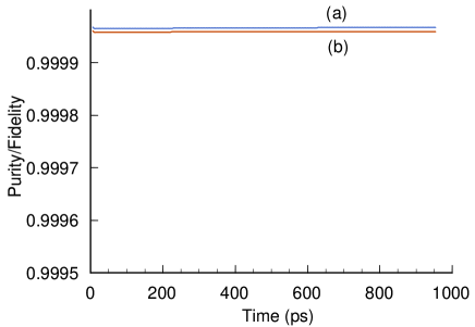
Figure 3: Time evolution of the purity (a) of the electron spin state and the fidelity (b) of the quantum state transfer after photoexcitation for the case of favorable conditions.

In the unfavorable case, the magnitude of the electron-hole exchange interaction ($W=20\;\mu$ eV) is rather large and the hole tunneling time ($1/t_{12}=1/t_{23}=$10 ps) is not short enough to suppress the spin state mixing by the electron-hole exchange interaction. In this case also, results are not sensitive to the polarization angle of the excitation light and are exhibited in Fig. 4. The purity decreases rapidly within several tens of picoseconds after photoexcitation due to the electron-hole exchange interaction. The characteristic time scale is given by $\hbar/W$ and is 33 ps. Then the purity is decreasing slowly due to the electron spin decoherence itself ($\sim 1\;\mu$s).

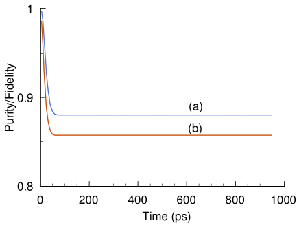
Figure 4: Time evolution of the purity (a) of the electron spin state and the fidelity (b) of the quantum state transfer after photoexcitation for the case of unfavorable conditions.

We also examined the fidelity of the quantum state transfer. Ideally we want to prepare the electron spin state corresponding to the photon polarization state in Eq. (9) as

$$\rho_{{\rm electron}}^{0}=\cos^{2}\theta|e_{1}\rangle\langle e_{1}|+\sin^{2}\theta|e_{2}\rangle\langle e_{2}|+i\sin\theta\cos\theta|e_{2}\rangle\langle e_{1}|-i\sin\theta\cos\theta|e_{1}\rangle\langle e_{2}|\;.$$ (21)

The fidelity is defined by

$${\cal F}(t)={\rm Tr}\;\rho_{{\rm electron}}^{0}\;\rho_{{\rm electron}}(t)\;,$$ (22)

where $\rho_{{\rm electron}}(t)$ is the reduced density matrix of the electron defined in Eq. (18). This quantity indicates to what extent the actual state is close to the ideally prepared state. The results are exhibited by curves (b) in Figs. 3 and 4. Qualitative features are the same as in the case of purity.

Based on these results, we can conclude that for the secure quantum state transfer we have to extract the photoexcited hole quickly before the spin state mixing sets in due to the electron-hole exchange interaction. The model used here has an empirical character and a more quantitative analysis would be necessary for the definite design of experiments of quantum state transfer[24, 25].

3 QUANTUM CORRELATION (Bell) MEASUREMENT BETWEEN TWO ELECTRONS

In the scheme of quantum repeater, the primary elements are the quantum state transfer between a photon and an electron and the entanglement swapping through the Bell (correlation) measurement between two electrons which are created through the quantum state transfer from two photons. It is preferable to do the Bell measurement between electrons instead of photons because the mismatch between the photon arrival times can be compensated by the rather long coherence time of electrons, whereas the storage of photons is rather difficult although the techniques for the photon storage are progressing steadily. Thus we start the discussion assuming that two electrons are prepared in a semiconductor nanostructure, e.g., a quantum dot. We propose an optical method to measure the spin state of two electrons based on the Faraday or Kerr rotation. Here we employ a linearly polarized off-resonant probe light and measure the orientation of the transmitted (reflected) light. Thus the method can be non-destructive in the same sense as demonstrated for the case of a single electron[26, 27].

Before going into details, let us review briefly the elementary processes of the Faraday rotation for the case of a single electron. We consider a III-V semiconductor quantum dot in which the hole ground state is the heavy hole state and a magnetic field is applied along the crystal growth direction (namely, perpendicular to the quantum well plane). As is well known, the right-circularly polarized light denoted by $\sigma_{+}$ excites a down spin electron from the valence band state $|3/2,-3/2\rangle$ creating a charged exciton or trion, while the left-circularly polarized light denoted by $\sigma_{-}$ excites an up spin electron from the valence band state $|3/2,3/2\rangle$, as exhibited in Fig. 5. When we probe the system with a linearly polarized light along the $x$ direction, i.e.,

$$|x\rangle=\frac{1}{\sqrt{2}}(|\sigma_{+}\rangle+|\sigma_{-}\rangle)\;,$$ (23)

one of the circular components receives a phase shift and the Faraday rotation occurs. Thus we can distinguish the two spin states of an electron by the sign of the Faraday rotation angle.

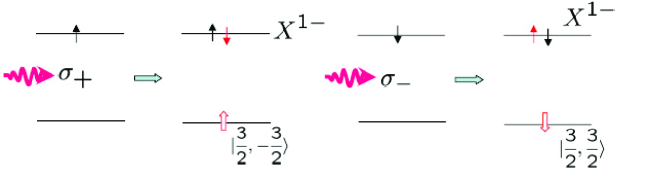
Figure 5: Elementary processes of the Faraday rotation for the case of a single resident electron. $\sigma_{+(-)}$ denotes the right (left) circularly polarized light. The upper (lower) horizontal line indicates the electron (hole) level. A thin (thick empty) arrow represents an electron (a hole) with the spin direction along the arrow.

Now we extend this argument to the case of two electrons and consider relevant elementary processes for four states of two electrons, namely, the singlet state(S) and the triplet states with the magnetic quantum number 1, 0 and -1 ($T_{1},T_{0},T_{-1}$). For the $T_{1}$ state, spins of the two resident electrons are aligned in the same direction and a $\sigma_{+}$ polarized light excites a down spin electron from the valence band creating a doubly negatively charged exciton $X^{2-}$, as shown in Fig. 6, in which the lowest electron orbital state is occupied by a spin-singlet electron pair and the spin direction of the electron in the second lowest orbital state is indicated in the superscript and the spin direction of the hole is depicted in the subscript. This $T_{1}$ state is optically inactive for the $\sigma_{-}$ polarized light. For the $T_{-1}$ state, a $\sigma_{-}$ polarized light excites an up spin electron from the valence band creating another doubly negatively charged exciton. This $T_{-1}$ state is optically inactive for the $\sigma_{+}$ polarized light. Thus these two states can be distinguished by the sign of the Faraday rotation angle. On the other hand, the S and $T_{0}$ states are optically active for both circular polarizations as exhibited in Figs. 7 and 8, and the sign of the Faraday rotation angle is determined by the competition between the phase shifts for each circular component.

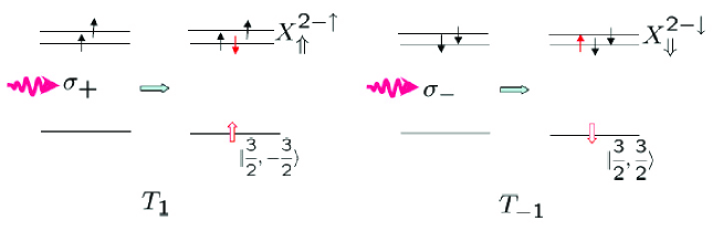
Figure 6: Elementary processes of the Faraday rotation for the triplet $T_{1}$ and $T_{-1}$ states of two resident electrons.

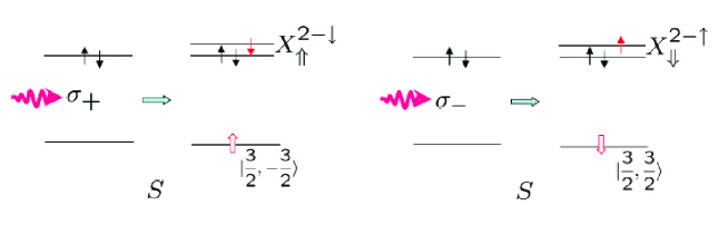
Figure 7: Elementary processes of the Faraday rotation for the singlet $S$ state of two resident electrons.

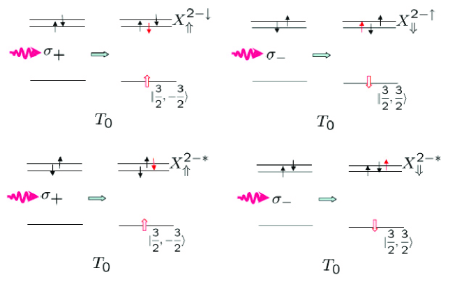
Figure 8: Elementary processes of the Faraday rotation for the triplet $T_{0}$ state of two resident electrons. $X_{\Uparrow}^{2-*}$ and $X_{\Downarrow}^{2-*}$ denote excited states of the doubly negatively charged exciton.

The expression of the Faraday rotation angle is obtained in the perturbation theory and is composed of two terms:

$$\varphi\propto\sum_{j(\sigma+)}\frac{|\langle j|P_{\sigma+}|i\rangle|^{2}(E_{j,i}-\hbar\omega)}{(\hbar^{2}\gamma^{2}_{j,i}+(E_{j,i}-\hbar\omega)^{2})}-\sum_{k(\sigma-)}\frac{|\langle k|P_{\sigma-}|i\rangle|^{2}(E_{k,i}-\hbar\omega)}{(\hbar^{2}\gamma^{2}_{k,i}+(E_{k,i}-\hbar\omega)^{2})}\;,$$ (24)

where $i$ indicates the initial state of two electrons, $j\;(k)$ the final state of the optical transition for the $\sigma_{+}\;(\sigma_{-})$ component, $E_{a,b}=E_{a}-E_{b}$ with $E_{a}$ being the energy of the $a$ state, $\gamma_{a,b}$ the dephasing rate corresponding to the $a\leftrightarrow b$ transition and $\hbar\omega$ denotes the photon energy of the linearly polarized probe light. As mentioned before, for the $T_{1}$ state only the $\sigma_{+}$ transitions contribute, whereas for the $T_{-1}$ state only the $\sigma_{-}$ transitions contribute. Thus the two states can be distinguished by the sign of the Faraday rotation angle. For the S and $T_{0}$ states, both $\sigma_{+}$ and $\sigma_{-}$ transitions contribute and thus more detailed arguments are necessary to determine the sign of the Faraday rotation angle. Now we examine the resonance position of the Faraday rotation angle with respect to the probe photon energy $\hbar\omega$. From the elementary processes exhibited in Figs. 6-8, it is seen that for the triplet states the resonance occurs at around the energy of the doubly charged exciton states ($E(X^{2-})$). On the other hand, for the singlet state the resonance occurs at a higher energy than $E(X^{2-})$ because the lowest orbital state is already occupied by a spin-singlet electron pair and the optical transition should occur to the higher orbital state.

Now we discuss more details of the Faraday rotation angle for the case of $T_{0}$ state. As mentioned before, both $\sigma_{+}$ and $\sigma_{-}$ circular components contribute to the Faraday rotation. The lowest-energy final state of the optical transition for each circular component is given by

$$j(\sigma+)=X^{2-\downarrow}_{\Uparrow}\;,\qquad k(\sigma-)=X^{2-\uparrow}_{\Downarrow}\;.$$ (25)

The energies of these states are different in a magnetic field because the spin configuration is different for these states. In terms of the electron $g$-factor $g_{c(v)}$ for the conduction (valence) band, these energies are given as

$$E(X^{2-\downarrow}_{\Uparrow})\cong-\frac{1}{2}(g_{c}\mu_{B}B-g_{v}\mu_{B}B)+E_{0}\;,$$ (26)

$$E(X^{2-\uparrow}_{\Downarrow})\cong\frac{1}{2}(g_{c}\mu_{B}B-g_{v}\mu_{B}B)+E_{0}\;,$$ (27)

where $E_{0}$ is the lowest energy of the interband transition. Then the energy difference $|E(X^{2-\downarrow}_{\Uparrow})-E(X^{2-\uparrow}_{\Downarrow})|$ is typically about one tenth of meV for a magnetic field about 1 Tesla and is comparable to the dephasing rate of the optical transitions. From the formula in Eq. (24) we see that the dependence of the Faraday rotation angle on the probe photon energy is determined by the difference between two dispersive curves with nearly equal resonance energies. Thus the profile is given by the derivative of the dispersive curve as shown in Fig. 9, depending on the sign of the energy difference. The same situation holds for the singlet state $S$.

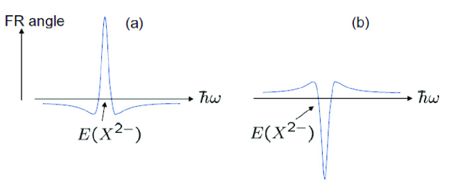
Figure 9: Dependence on the probe photon energy ($\hbar\omega$) of the Faraday rotation angle for the triplet $T_{0}$ state and the singlet $S$ state of two resident electrons. It depends on the sign of the energy difference; namely, (a) $|E(X^{2-\downarrow}_{\Uparrow})-E(X^{2-\uparrow}_{\Downarrow})|>0$, (b) $|E(X^{2-\downarrow}_{\Uparrow})-E(X^{2-\uparrow}_{\Downarrow})|<0$

Summarizing these considerations, we can show the schematic dependence of the Faraday rotation angle on the probe photon energy in Fig. 10. The triplet states $T_{1}$ and $T_{-1}$ exhibit a typical dispersive lineshape. On the other hand, the profile for the triplet $T_{0}$ and the singlet $S$ states is given by the derivative of the dispersive curve, where the case of $|E(X^{2-\downarrow}_{\Uparrow})-E(X^{2-\uparrow}_{\Downarrow})|>0$ is assumed. The resonance occurs at around the energy of the doubly charged exciton state denoted by $E(X^{2-})$ for the triplet states, whereas for the singlet state it occurs at a higher energy than $E(X^{2-})$ by the orbital excitation energy $\Delta_{e}$. Thus when we choose the probe photon energy at the downward arrow as shown in Fig. 10, the Faraday rotation angle is positive for the $T_{1}$ state and is negative for the $T_{-1}$ state. For the $T_{0}$ state, the Faraday rotation angle is negative but the magnitude is small. For the singlet $S$ state, the Faraday rotation angle would be vanishingly small because of the large off-resonance. Consequently, we can distinguish between the four states of two electrons by the magnitude and the sign of the Faraday rotation angle.

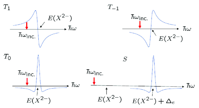
Figure 10: Dependence on the probe photon energy ($\hbar\omega$) of the Faraday rotation angle for the three triplet states $T_{1},T_{0},T_{-1}$ and the singlet state $S$ of two resident electrons. Those for $T_{0}$ and $S$ are exhibited for the case of $|E(X^{2-\downarrow}_{\Uparrow})-E(X^{2-\uparrow}_{\Downarrow})|>0$.

Now we discuss relevant parameters to optimize the Faraday rotation measurement. The essential requirement is the preparation of the lowest two orbital states which are energetically well-separated from higher excited states. We consider a circularly symmetric GaAs quantum dot with parabolic lateral confinement under a magnetic field along the growth direction. Then the orbital eigenstates are represented by the Fock-Darwin states[28, 29] whose eigenenergies are given by

$$E_{\nu,n}=(|n|+1+2\nu)\hbar\Omega+\frac{n}{2}\hbar\omega_{c}$$ (28)

$${\rm with}\;\; \Omega=\sqrt{\omega^{2}_{0}+\frac{\omega^{2}_{c}}{4}}\;,\;\omega_{c}=\frac{eB}{m^{*}c}\;,$$ (29)

where $\omega_{0}$ is the frequency of the harmonic confinement in the lateral direction and $m^{*}$ is the electron effective mass. When we employ the parameter values: $\hbar\omega_{0}=5$meV, $B=5$T and $m^{*}=0.067m_{0}$ with $m_{0}$ being the free electron mass, we have $\hbar\omega_{c}=8.7$meV and $\hbar\Omega=6.63$meV. The lowest two orbital levels have the spacing of 2.3 meV and are well-separated from the higher orbital level by 8.7 meV. These parameter values would enable the Faraday rotation measurement to be carried out reliably.

4 DYNAMICS IN ELECTRON-NUCLEI COUPLED SYSTEM

As mentioned in Sec. 1, the electron spin decoherence time reported so far for low temperatures is about a few microsecond and is not sufficiently long for the secure quantum information processing. Here the hyperfine (HF) interaction with the host nuclei[30, 31] is considered to be the main decoherence mechanism, dominating over spin-orbit interactions which act on a time scale of tens of milliseconds[32, 33] or even longer. Consequently there have been proposals to reduce the HF induced decoherence by measuring or polarizing the nuclear spins[34, 35, 36, 37, 38] and to use nuclear spins as a quantum memory[39].

Extending these studies, we investigate the electron-nuclei spin coupling in quantum dots (QDs) and show that consecutive measurements of the electron spin state following the HF interaction are correlated and lead to purification of the nuclear spin system. More specifically, starting from an unknown initial state of nuclear spins, successive measurements of the electron spin state result in narrowing of the distribution of the nuclear spin field. We predict that the purification of the nuclear spin state would lead to the bunching of results of the electron spin state measurements and also to the reduction in the electron spin decoherence induced by the HF interaction. For the physical realization of the proposals we will in particular discuss a double QD occupied by two electrons, and a single QD occupied by one or two electrons. Under sufficiently high magnetic fields compared with the effective HF field (Overhauser field), these systems provide the desired two-level system with a unidirectional HF field.

First of all we consider an electrically gated double QD occupied by two electrons[18, 40]. The excited electronic orbitals of QDs have an energy much greater than the thermal energy and the adiabatic voltage sweeping rates, so that the electrons occupy only the ground state orbitals. Under a high magnetic field where the electron Zeeman splitting is much greater than the HF fields and the exchange energy, dynamics takes place in the spin singlet ground state $|S\rangle$ and triplet state of zero magnetic quantum number $|T\rangle$. For the singlet state each electron can be found in the different QD or both in the same QD, whereas for the triplet state electrons can only be found in different QDs. In order to derive the effective Hamiltonian for the singlet and triplet states of two electrons each of which is lying in a different QD, we rewrite the HF interaction for two electrons in the bases of singlet and triplet states and find that the mean HF field induces mixing within triplet states and the difference of the HF fields in two QDs induces coupling between the singlet and triplet states. When the Zeeman energy is much larger than the HF fields, the coupling terms among the triplet states and those between $|T_{\pm}\rangle$ (triplet states with the magnetic quantum number of 1 or -1) and the singlet state $|S\rangle$ can be neglected and the HF interaction reduces to

$$V_{HF}=\delta h_{z}(|S\rangle\langle T|+{\tt h.c.})/2$$ (30)

with $\delta h_{z}=h_{Lz}-h_{Rz}$ being the difference of the HF fields along the applied field direction in the left and right QDs. Including the exchange energy splitting $J$ between $|S\rangle$ and $|T\rangle$, the effective Hamiltonian is given as

$$H_{e}=JS_{z}+r\delta h_{z}S_{x}\;,$$ (31)

where ${\bf S}$ is the pseudospin operator with $|T\rangle$ and $|S\rangle$ forming the $S_{z}$ basis and the parameter $r$ characterizes the hybridization ratio of the singlet state whose two electrons are separated in different QDs in the true singlet ground state. When both electrons are localized in the same dot, $r\rightarrow 0$ and $J\gg\delta h_{z}$. On the other hand, when they are located in different dots, the HF coupling is maximized $r\rightarrow 1$ and $J\rightarrow 0$.

In the following we develop the arguments based on Eq. (31) assuming that the time scale of the nuclear spin variation is much longer than that of the electron spin measurements. Thus we take into account only the static(inhomogeneous) distribution of the nuclear Overhauser field but not the dynamical motion of the nuclear spin system itself due to the dipole-dipole interaction which would induce additional decoherence of the electron spins.

4.1 Bunching in electron spin measurements

Now we show that by electron spin measurements in a double QD governed by Eq. (31), the coherent behavior of nuclear spins can be demonstrated. Electron spins are initialized in the singlet state and the nuclear spin states are initially in a mixture of $\delta h_{z}$ eigenstates:

$$\rho(t=0)=\sum_{n}p_{n}\;\rho_{n}\;|S\rangle\langle S|\;,$$ (32)

where $\rho_{n}$ is a nuclear eigenstate with an eigenvalue $h_{n}$:

$${\rm Tr}\;\rho_{n}\;\delta h_{z}=h_{n}\>,\quad{\rm Tr}\;\rho_{n}=1\;.$$ (33)

$p_{n}$ is the probability of the hyperfine field $\delta h_{z}$ having the value $h_{n}$. In the unbiased regime $r=1$, the nuclear spins and the electron spins interact for a time span of $t$. The time evolution of the system is described as follows:

$$\rho(t=0)=\sum_{n}p_{n}\rho_{n}\;|S\rangle\langle S|\rightarrow\rho(t)=\sum_{n}p_{n}\rho_{n}\;|\Psi_{n}\rangle\langle\Psi_{n}|\;,$$ (34)

$$|\Psi_{n}\rangle=\alpha_{n}(t)|S\rangle+\beta_{n}(t)|T\rangle\;,$$ (35)

$$\alpha_{n}(t)=\cos\Omega_{n}t/2+iJ/\Omega_{n}\sin\Omega_{n}t/2\;,\;\beta_{n}(t)=-ih_{n}/\Omega_{n}\sin\Omega_{n}t/2\;,$$ (36)

$$\Omega_{n}=\sqrt{J^{2}+h_{n}^{2}}\;.$$ (37)

Then the gate voltage is swept adiabatically, switching off the HF interaction $r\rightarrow 0$, in a time scale much shorter than HF interaction time. Next a charge state measurement is performed which detects a singlet or triplet state. Probability to detect the singlet state is

$$P_{S}(t)={\rm Tr}_{{\rm nuc.}}\langle S|\rho(t)|S\rangle=\sum_{n}p_{n}|\alpha_{n}|^{2}\;,$$ (38)

where the nuclear states are traced out because they are not observed. In the same way the probability to detect the triplet state is

$$P_{T}(t)=\sum_{n}p_{n}|\beta_{n}|^{2}\;.$$ (39)

After the first measurement, assuming that the outcome is the singlet, the system is in the state given by

$$\frac{1}{P_{S}(t)}\sum_{n}p_{n}|\alpha_{n}|^{2}\rho_{n}|S\rangle\langle S|\;,$$ (40)

where $P_{S}(t)$ in the denominator is the normalization constant of the density matrix. In the second run we again initialize the system in the spin singlet state of the two electrons, preparing the state:

$$\rho^{\prime}(t=0)=\frac{1}{P_{S}(t)}\sum_{n}p_{n}|\alpha_{n}|^{2}\rho_{n}\;|S\rangle\langle S|$$ (41)

and turn on the HF interaction. After the same period $t$ as in the first run, the system evolves to

$$\rho^{\prime}(t)=\frac{1}{P_{S}(t)}\sum_{n}p_{n}|\alpha_{n}|^{2}\rho_{n}\;|\Psi_{n}\rangle\langle\Psi_{n}|$$ (42)

$$|\Psi_{n}\rangle=\alpha_{n}(t)|S\rangle+\beta_{n}(t)|T\rangle\;,$$ (43)

where $\alpha_{n}(t)$ and $\beta_{n}(t)$ are given in Eq. (36). Then the probability to detect the singlet state in the second measurement $P_{SS}(t;t)$, where the first (second) subscript represents the outcome of the first (second) measurement, is given by

$$P_{SS}(t;t)=P_{S}(t)\cdot{\rm Tr}_{{\rm nuc.}}\langle S|\rho^{\prime}(t)|S\rangle=\sum_{n}p_{n}|\alpha_{n}|^{4}\;,$$ (44)

where it is to be noted that the probability $P_{S}(t)$ of the first measurement cancels the normalization factor in Eq. (42). In the same way the probability to detect the triplet state in the second measurement $P_{ST}(t;t)$ is given by

$$P_{ST}(t;t)=\sum_{n}p_{n}|\alpha_{n}|^{2}|\beta_{n}|^{2}\;.$$ (45)

After the second measurement, assuming that the first (second) outcome is the singlet (triplet), the system is in the state given by

$$\frac{1}{P_{ST}(t;t)}\sum_{n}p_{n}|\alpha_{n}|^{2}|\beta_{n}|^{2}\rho_{n}\;|T\rangle\langle T|\;,$$ (46)

where $P_{ST}(t;t)$ in the denominator is the normalization factor of the density matrix. In this way we can repeat many times of measurements.

In general over $N$ measurements, the nuclear state conditioned on $k\;(\leq N)$ times singlet and $N-k$ times triplet detection is

$$\sigma_{N,k}=\bigl{(}^{N}_{\,k}\bigr{)}\sum_{n}p_{n}|\alpha_{n}|^{2k}|\beta_{n}|^{2(N-k)}\rho_{n}\;,$$ (47)

the trace of which yields the probability of $k$ times singlet outcomes

$$P_{N,k}={\rm Tr}\;\sigma_{N,k}=\bigl{(}^{N}_{\,k}\bigr{)}\langle|\alpha|^{2k}|\beta|^{2(N-k)}\rangle\;,$$ (48)

where $\langle\ldots\rangle$ is the ensemble averaging over the hyperfine field $h_{n}$[31]. Hereafter, this case will be referred to as the coherent regime. One can contrast this regime with the incoherent regime in which nuclear spins lose their coherence between the successive spin measurements and relax to the equilibrium distribution. The result for the latter regime is given by

$$P^{\prime}_{N,k}=\bigl{(}^{N}_{\,k}\bigr{)}\langle|\alpha|^{2}\rangle^{k}\langle|\beta|^{2}\rangle^{(N-k)}\;.$$ (49)

In the following we assume that the initial nuclear spins are unpolarized and randomly oriented and thus the distribution of the hyperfine field is characterized by a Gaussian distribution with variance $\sigma^{2}$:

$$p[h]=\frac{1}{\sqrt{2\pi\sigma^{2}}}e^{-\frac{h^{2}}{2\sigma^{2}}}\;.$$ (50)

The summation is converted to an integration:

$$\sum_{n}\;p_{n}\ldots\rightarrow\int{\tt d}h\,p[h]\ldots\;.$$ (51)

As the simplest case, let us examine the results for two ($N=2$) measurements, each following a HF interaction of duration time $t$. The probability for two consecutive singlet detections is given by

$$P_{2,2}=\langle|\alpha|^{4}\rangle=\{6+2e^{-2\bar{t}^{2}}+8e^{-\bar{t}^{2}/2}\}/16$$ (52)

for the coherent regime with $\bar{t}=\sigma t$ and this is always greater than

$$P^{\prime}_{2,2}=\langle|\alpha|^{2}\rangle^{2}=\{4+8e^{-\bar{t}^{2}/2}+4e^{-\bar{t}^{2}}\}/16$$ (53)

for the incoherent regime. These results are given particularly for $J=0$. As $J$ is increased the probabilities approach each other and for $J\gg\sigma$ they become identical[41].

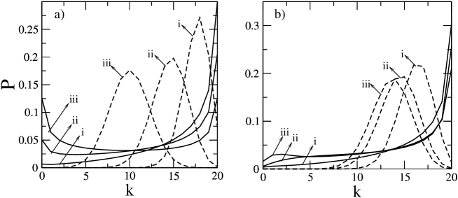
Figure 11: Probability distribution for $N=20$ measurements as a function of times ($k$) of singlet detections, for coherent regime (solid lines) and incoherent regime (dashed lines). Two cases of the exchange energy are considered a) $J=0$ , and b) $J/\sigma=0.5$ , for HF interaction times $\sigma\tau=$ i) $0.5$, ii) $1.5$, and iii) $\infty$.

In Fig. 11, for $N=20$ measurements, $P_{N,k}$ and $P^{\prime}_{N,k}$ are shown for HF interaction times $\sigma\tau=0.5,1.5,{\rm and}\;\infty$. For $\tau=0$, both probabilities are peaked at $k=20$. However, immediately after the HF interaction is introduced, the probability distributions show distinct behavior. The measurement results in the incoherent regime approach a Gaussian distribution. In the coherent case the probabilities bunch at $k$=0 and 20 for $J=0$, and when $J/\sigma=0.5$ those bunch at $k=20$ only. As $J$ is increased above some critical value, no bunching takes place at $k=0$ singlet measurement. When $J$ is finite, the singlet state is energetically favored and the bunching of the singlet state outcome is more probable. Thus if the nuclear spins are coherent over the span of the experiment, successive electron spin measurements are likely to be biased to all singlet or triplet outcomes.

We discuss in brief the feasibility to observe the predicted phenomenon. The duration of the cycle involving electron spin initialization and measurement is about $10~{}\mu$s[18]. The nuclear spin coherence time determined mostly by the nuclear spin diffusion is longer than about several tens of ms[42]. For a HF interaction of duration $\tau=4\sigma^{-1}\sim 40\mu$s [18] in each step, the bunching can be observed for $N$ successive measurements up to $N\sim 200$.

4.2 Purification of nuclear spin state and revival of the initial electron state

The nuclear spin state conditioned on the previous electron spin measurements is no longer random even if they are initially random. To be stated in more detail, the quantum correlation is built up in the nuclear spin system as a consequence of back-actions of the electron spin measurements. This quantum correlation affects in turn the outcomes of the electron spin measurements. In order to examine this situation, we consider the case: Starting from a random spin configuration, $N$ successive electron spin measurements are performed, each following initialization of electron spins in the spin singlet state and a HF interaction of duration $\tau_{i}$ ($i=1\ldots N$) and all the outcomes turn out to be the singlet. Then again the HF interaction is switched on for a time $t$, and the $(N+1)$-th measurement is carried out. The conditional probability to recover the initial state, namely to observe again the singlet state, is given by

$$P(t)=\frac{\sum\prod_{i=1}^{N+1}\binom{2}{s_{i}}e^{-\frac{1}{2}\bigl{[}\sum_{j=1}^{N}(s_{j}-1)\bar{\tau}_{j}+(s_{N+1}-1)\bar{t}\bigr{]}^{2}}}{4\sum\prod_{i=1}^{N}\binom{2}{s_{i}}e^{-\frac{1}{2}\bigl{[}\sum_{j=1}^{N}(s_{j}-1)\bar{\tau}_{j}\bigr{]}^{2}}}\;,$$ (54)

where the sums run over $s_{i}=0,1,2$ and $\bar{\tau}_{i}=\sigma\tau_{i}$. For the particular case of $\tau_{1}=\tau_{2}=\ldots=\tau_{N}=\tau\gg 1/\sigma$, Eq. (54) can be approximated as

$$P(t)\simeq 1/2+\sum_{s=0}^{N}(^{2N}_{~{}s})e^{\frac{-\sigma^{2}}{2}(t-(N-s)\tau)^{2}}/2(^{2N}_{~{}N})\quad{\rm for}\;\tau\gg 1/\sigma\>.$$ (55)

This indicates a periodical recurrence of the initial state of the electron spin. Indeed the initial state is revived at $t=n\tau,\,(n=1,2,\ldots,N)$ with a decreasing amplitude:

$$1/2+\binom{2N}{N-n}/2\binom{2N}{N}\;.$$ (56)

In Fig. 12 the conditional probabilities in Eq. (54) are shown for $\sigma\tau=1.0,3.0,6.0$ subject to $N=0,1,2,5,10$ times prior singlet measurements in each. Revivals or recurrences are observable only for $\sigma\tau>1$, because the modulation period of the nuclear field spectrum characterized by $1/\tau$ should be smaller than the variance $\sigma$, as will be explained later.

In order to understand the mechanism of revivals, we examine the purity of the nuclear spin system. The purity of a system characterized by the density matrix $\rho$ is given by

$${\cal P}={\rm Tr}\;\rho^{2}\;.$$ (57)

We consider the nuclear spin state prepared by $N$ successive electron spin measurements in which all the outcomes are the singlet and the duration times of the HF interaction are $\tau_{1},\cdots,\tau_{N}$. The purity of this nuclear spin state is calculated as

$${\cal P}=\frac{1}{\cal D}\frac{\sum_{s_{i}=0}^{4}\prod_{i=1}^{N}\binom{4}{s_{i}}e^{-\frac{1}{2}\bigl{[}\sum_{j=1}^{N}(s_{j}-2)\bar{\tau}_{j}\bigr{]}^{2}}}{\bigl{[}\sum_{s_{i}=0}^{2}\prod_{i=1}^{N}\binom{2}{s_{i}}e^{-\frac{1}{2}\bigl{[}\sum_{j=1}^{N}(s_{j}-1)\bar{\tau}_{j}\bigr{]}^{2}}\bigr{]}^{2}}\;,$$ (58)

where ${\cal D}$ is the dimension of the Hilbert space for the nuclear spins. For a fixed ratio of $\tau_{1}:\tau_{2}:\ldots:\tau_{N}$, the purity in Eq. (58) is a monotonically increasing function of time. For $\bar{\tau}_{i}=\sigma\tau_{i}\gg 1$, one can attain various asymptotic limits for the purity. For instance, for $N=2$, there are three asymptotic limits:

a) $\tau_{1}=2\tau_{2}$

$${\cal P}=11/4{\cal D}\;,$$ (59)

b) $\tau_{1}=\tau_{2}$

$${\cal P}=35/18{\cal D}\;,$$ (60)

c) otherwise

$${\cal P}=9/4{\cal D}\;.$$ (61)

For $N=2$ with $\tau_{1}=2\tau_{2}=2\tau\gg 1/\sigma$, the conditional probability in Eq. (54) is given as

$$P(t)\simeq 1/2+\sum_{n=0}^{3}(4-n)\exp[-(\bar{t}-n\bar{\tau})^{2}/2]/8\;,$$ (62)

whereas for $\tau_{1}=\tau_{2}=\tau\gg 1/\sigma$,

$$P(t)\simeq 1/2+\bigl{\{}e^{-\frac{(\bar{t}-2\bar{\tau})^{2}}{2}}+4e^{-\frac{(\bar{t}-\bar{\tau})^{2}}{2}}+6e^{-\frac{\bar{t}^{2}}{2}}\bigr{\}}/12\;.$$ (63)

It can be seen that as the purity of nuclear spins increases, more revivals are present with an increased amplitude. Thus we can conclude that the mechanism of the revival phenomenon is the purification of the nuclear spin system through the electron state measurements.

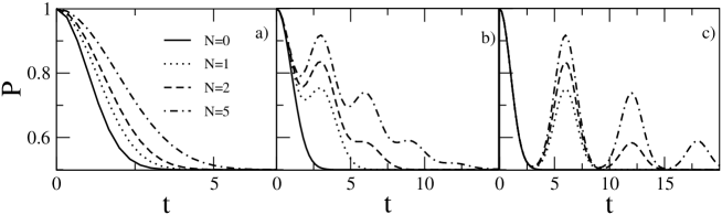
Figure 12: Conditional probability for singlet state detection as a function of HF interaction time $\sigma t$, subject to $N=0,1,2,5,10$ times prior singlet state measurements and for HF interaction times of a) $\sigma\tau=1.0\;$, b) $\sigma\tau=3.0\;$, and c) $\sigma\tau=6.0\;$.

Previously, various methods have been proposed in order to control the nuclear spin system. A typical method is based on measurement of the HF field in a QD with some precision[36, 37, 38]. In the method proposed here, on the other hand, the nuclear spin state can be conditionally purified without determining the precise value of the HF field. Although the HF field is still assuming various values, the quantum correlation is built up, leading to the revival phenomenon. In order to understand these features clearly, we simplify the situation by putting $J=0$ in Eq. (36). Then the nuclear state density matrix, after $N$ times electron spin measurements with all the outcomes being the singlet, is given by

$$\rho_{nuc.}\propto\sum_{n}p_{n}|\cos h_{n}\tau/2|^{2N}\rho_{n}$$ (64)

and the corresponding nuclear field spectrum or distribution function assumes a form of

$$p[h]={\cal N}e^{-h^{2}/2\sigma^{2}}\cos^{2N}[h\tau/2]\;,$$ (65)

where ${\cal N}$ is an appropriate normalization constant. Thus the modulation period of the nuclear field spectrum is characterized by $1/\tau$. When this modulation period is larger than the width $\sigma$ of the initial Gaussian distribution, i.e., $\sigma\tau<1$, the effect of modulation is not manifest. This explains the absence of revivals in Fig. 12 a).

Since the absolute value of a cosine function is less than unity, many times multiplication of the cosine function leads to sharpening of the distribution. Indeed, we can approximate for $N\gg 1$ as

$$\cos^{2N}\theta=\sum_{s\in\mathbb{Z}}(1-\frac{1}{2}(\theta-s\pi)^{2}+\cdots)^{2N}$$ (66)

$$\hskip 34.14322pt=\sum_{s\in\mathbb{Z}}(1-N(\theta-s\pi)^{2}+\cdots)\simeq\sum_{s\in\mathbb{Z}}\exp[-N(\theta-s\pi)^{2}]\;.$$ (67)

Then Eq. (65) can be cast into a series of very narrow Gaussian functions

$$p[h]={\cal N}e^{-h^{2}/2\sigma^{2}}\cos^{2N}[h\tau/2]\simeq{\cal N}e^{-h^{2}/2\sigma^{2}}\sum_{s\in\mathbb{Z}}e^{-(h-h_{s})^{2}/2\sigma_{m}^{2}}$$ (68)

$$\sigma_{m}^{-1}=\tau\sqrt{N/2}\;,\;h_{s}=2s\pi/\tau\;,$$ (69)

where it is to be noted that the width of Gaussians is inversely proportional to $\sqrt{N}$. Thus the nuclear field distribution function is squeezed by successive electron spin measurements and this is the origin of increase in the purity of the nuclear state. Then the probability to have a singlet outcome in the $(N+1)$-th measurement after the HF interaction of period $t$ is calculated as

$$P(t)=\langle\cos^{2}ht/2\rangle={\cal N}\int dh\;\cos^{2}(ht/2)\;e^{-h^{2}/2\sigma^{2}}\sum_{s\in\mathbb{Z}}e^{-(h-h_{s})^{2}/2\sigma_{m}^{2}}$$ (70)

$$\hskip 82.51282pt=\frac{1}{2}+\frac{\cal N}{2}\;\sum_{s\in\mathbb{Z}}e^{-\sigma_{m}^{2}t^{2}/2}e^{-h_{s}^{2}/2\sigma^{2}}\cos h_{s}t\;.$$ (71)

At $t=n\tau$, all $\cos h_{s}t$ terms add up constructively leading to the revival phenomenon, namely, a high probability to observe the spin singlet state periodically.

So far we have discussed the case in which the initial state of the electron pair is the singlet. But these arguments can be extended to the case of an arbitrary initial state. When the initial state of the electron pair is prepared as

$$\Psi(t=0)=\cos\frac{\theta}{2}|S\rangle+\sin\frac{\theta}{2}e^{-i\phi}|T\rangle\;,$$ (72)

the probability to recover the initial state $\Psi(t=0)$ at time $t$ is calculated as

$$F={\rm Tr}_{{\rm nuc.}}\langle\Psi(t=0)|\rho(t)|\Psi(t=0)\rangle$$ (73)

$$\hskip 10.81218pt=\sin^{2}\theta\cos^{2}\phi+(1-\sin^{2}\theta\cos^{2}\phi)P(t)$$ (74)

with $P(t)$ given by Eq. (54). Thus the recurrence phenomenon can be observed for an arbitrary initial state of the electron pair.

Finally, as an example, we consider the case when the nuclear spin state is prepared by five HF interaction stages each of which has duration $\tau=10/\sigma$ and is followed by a singlet detection of the electron spin state. This conditionally prepared nuclear spin state revives the initial electron state at $t=s\tau\;(s=1,2,\ldots,5)$ with the probability of $11/12,31/42,\ldots,253/504$, respectively. Success probability to prepare such a state is $\sim 1/32$. Here preparation time is $T=N(\tau+\tau_{w})$ where $\tau_{w}$ is the time needed for initialization and detection of the electron spin. During the HF interaction time $\tau$, phonon-mediated interations which act on the time scale longer than millisecond [33] or any other electron spin decoherence mechanism except the HF interaction should not take place. Furthermore the preparation time $T$ should be smaller than the nuclear diffusion time which is of the order of 10 ms[42]. Typically $\tau_{w}=10\;\mu$s, and let $\sigma^{-1}=10\;\mu$s[18]. For the discussed example ($\tau=10/\sigma$, $N=5$), the time needed for preparation of the desired nuclear spin state is $T=550\;\mu$s which is shorter than the nuclear spin diffusion time.

4.3 Extension to general situations

We have so far discussed the bunching and revival phenomena only for two electrons in a double QD system. The same predictions can also be made for a single QD occupied by a single electron. Consider a single QD occupied by a single electron[43, 44, 45], under an external magnetic field where the electron Zeeman energy is much greater than the HF energies. Then the system is described by the Hamiltonian:

$$H\simeq g_{e}\mu_{B}BS_{z}+h_{z}S_{z}\;,$$ (75)

where $S_{z}$ is the $z$ component of the electron spin operator, $g_{e}$ the electron $g$-factor, $\mu_{B}$ the Bohr magneton and $B$ is the external magnetic field applied in the $z$ direction. Spin flips are suppressed since

$$g_{e}\mu_{B}B\gg\sqrt{\langle{\bf h}^{2}\rangle}\;.$$ (76)

The spin eigenstates along the $x$ direction are given by

$$|\pm\rangle=(|\uparrow\rangle\pm|\downarrow\rangle)/\sqrt{2}\;,$$ (77)

where $|\uparrow\rangle$ and $|\downarrow\rangle$ are the eigenstates of $S_{z}$ and they are coupled via the HF interaction. Thus the relevant Hamiltonian in the basis of $|\pm\rangle$ is

$$H=\left(\begin{array}[]{cc}|+\rangle&|-\rangle\\ 0&(g_{e}\mu_{B}B_{z}+h_{z})/2\\ (g_{e}\mu_{B}B_{z}+h_{z})/2&0\end{array}\right)\;.$$ (78)

Then the spin state measurement is carried out as follows. Each time the electron is prepared in the $|+\rangle$ state. Next it is loaded onto the QD, then removed from the QD after some dwelling time $\tau$. The spin measurement is performed in the $|\pm\rangle$ basis. Essentially the same predictions can be made for this system as those for the case of double QD, namely the electron spin bunching and revival.

We can extend the arguments also to the case of a pair of electrons in a single QD[46, 47] as the Hamiltonian (31) can be used to describe the dynamics. Consequently, the same predictions as those for a double QD can be made[41]. Now we derive the Hamiltonian for an electron pair in a single QD. Under a sufficiently strong magnetic field, the triplet states $T_{\pm}$ with the magnetic quantum number of $\pm 1$ are well separated from the triplet $T_{0}$ state and the singlet state $S$. Thus the Hamiltonian within the subspace spanned by $T_{0}$ and $S$ states will be considered. The wavefunctions for the $S$ and $T_{0}$ states are given, respectively, as

$$\Psi_{S}({\bf r}_{1},\xi_{1},{\bf r}_{2},\xi_{2})=\phi_{g}({\bf r}_{1})\phi_{g}({\bf r}_{2})\frac{1}{\sqrt{2}}(\alpha(\xi_{1})\beta(\xi_{2})-\beta(\xi_{1})\alpha(\xi_{2}))\;,$$ (79)

$$\Psi_{T_{0}}({\bf r}_{1},\xi_{1},{\bf r}_{2},\xi_{2})=\frac{1}{2}(\phi_{g}({\bf r}_{1})\phi_{e}({\bf r}_{2})-\phi_{e}({\bf r}_{1})\phi_{g}({\bf r}_{2}))$$

$$\hskip 85.35826pt\cdot(\alpha(\xi_{1})\beta(\xi_{2})+\beta(\xi_{1})\alpha(\xi_{2}))\;,$$ (80)

where $\phi_{g}\;(\phi_{e})$ is the ground (excited) orbital state in the QD and $\alpha\;(\beta)$ denotes the spin up (down) state. The HF interaction for two electrons is given by

$$V_{HF}=Av_{0}\sum_{i}{\bf S}_{1}\cdot{\bf I}_{i}\;\delta({\bf r}_{1}-{\bf r}_{i})+Av_{0}\sum_{i}{\bf S}_{2}\cdot{\bf I}_{i}\;\delta({\bf r}_{2}-{\bf r}_{i})\;,$$ (81)

where $A$ is the HF coupling constant, $v_{0}$ the volume of a unit cell, S (I) is the electron (nuclear) spin operator and the summation is carried out over nuclear spins at the location ${\bf r}_{i}$. Then we find

$$\langle\Psi_{T_{0}}|V_{HF}|\Psi_{S}\rangle=-\frac{1}{\sqrt{2}}Av_{0}\sum_{i}\phi_{e}^{*}({\bf r}_{i})\phi_{g}({\bf r}_{i})I_{iz}\;,$$ (82)

$$\langle\Psi_{S}|V_{HF}|\Psi_{T_{0}}\rangle=\langle\Psi_{T_{0}}|V_{HF}|\Psi_{S}\rangle^{*}\;,\langle\Psi_{S}|V_{HF}|\Psi_{S}\rangle=\langle\Psi_{T_{0}}|V_{HF}|\Psi_{T_{0}}\rangle=0\;.$$ (83)

Thus the singlet-triplet mixing is induced by the HF interaction. The effective nuclear field operator will be denoted by

$$h=-\frac{1}{\sqrt{2}}Av_{0}\sum_{i}\phi_{e}^{*}({\bf r}_{i})\phi_{g}({\bf r}_{i})I_{iz}$$ (84)

which has the dimension of energy and its mean square value is estimated as

$$\langle hh^{{\dagger}}\rangle=\frac{(Av_{0})^{2}}{2}\sum_{i}|\phi_{e}^{*}({\bf r}_{i})\phi_{g}({\bf r}_{i})|^{2}\langle I^{2}_{iz}\rangle$$ (85)

$$\hskip 27.03003pt=\frac{A^{2}v_{0}}{2}\frac{I(I+1)}{3}\int d^{3}r\;|\phi_{e}^{*}({\bf r})\phi_{g}({\bf r})|^{2}\;,$$ (86)

where $I$ is the magnitude of the nuclear spin. Employing the envelope functions for the ground and excited states given by

$$\phi_{g}(r,\theta,z)=\frac{1}{\sqrt{\pi}r_{0}}e^{-\frac{r^{2}}{2r_{0}^{2}}}\sqrt{\frac{2}{d}}\cos(\frac{\pi z}{d})\;,$$ (87)

$$\phi_{e}(r,\theta,z)=\frac{1}{\sqrt{\pi}r_{0}^{2}}e^{-\frac{r^{2}}{2r_{0}^{2}}}\;re^{-i\theta}\sqrt{\frac{2}{d}}\cos(\frac{\pi z}{d})\;,$$ (88)

$$r_{0}=\sqrt{\frac{\hbar}{m^{*}\Omega}}\;,\;\Omega=\sqrt{\omega^{2}_{0}+(\frac{eB}{2m^{*}c})^{2}}\;,$$ (89)

where $\omega_{0}$ is the frequency of the harmonic confinement in the lateral direction, $m^{*}$ the electron effective mass and $d$ is the thickness of the QD, we have

$$\langle hh^{{\dagger}}\rangle=\frac{A^{2}v_{0}}{16\pi r_{0}^{2}d}\;I(I+1)\;.$$ (90)

In the vicinity of the singlet/triplet crossing point, the relevant Hamiltonian is given by

$$H=\left(\begin{array}[]{cc}|S\rangle&|T_{0}\rangle\\ 0&h^{{\dagger}}\\ h&0\end{array}\right)\;,\quad h=-\frac{1}{\sqrt{2}}Av_{0}\sum_{i}\phi_{e}^{*}(\vec{r}_{i})\phi_{g}(\vec{r}_{i})I_{iz}\;.$$ (91)

Thus the same predictions of the bunching and revival phenomena as before can be made since the relevant Hamiltonian is the same.

5 SUMMARY

We have investigated theoretically the fundamental elements for realizing the quantum repeater based on photons as flying qubits and electrons as operation qubits in semiconductor nanostructures; namely, the quantum state transfer between a photon and an electron spin, the quantum correlation (Bell) measurement of two electrons and the electron-nuclei coupled dynamics whose understanding is indispensable to realize the nuclear spin quantum memory. For the first element, we have analyzed the performance of the quantum state transfer and clarified the conditions to be satisfied to achieve a high value of the purity of the transferred quantum state or the fidelity of the operation. For the second element, we proposed an optical method to distinguish between four states of two electrons based on the Faraday or Kerr rotation and confirmed the feasibility. For the third element, we studied the electron-nuclei coupled dynamics and predicted a couple of new phenomena related to the correlations induced by the hyperfine interactions. The underlying mechanism is the squeezing or the increase in the purity of the nuclear spin state through the electron spin measurements. We can construct hopefully a secure and robust system of the quantum repeater combining these results, namely, the efficient quantum state transfer between a photon and an electron spin, the reliable Bell measurement of two electrons for the entanglement swapping based on the Faraday or Kerr rotation and the long-lived quantum memory based on nuclear spins.

- [1] C. H. Bennett and D. P. DiVincenzo, “Quantum information and computation,” Nature 404, 247–255 (2000) [doi:10.1038/35005001].
- [2] A. Barenco, D. Deutsch, A. Ekert, and R. Jozsa, “Conditional quantum dynamics and logic gates,” Phys. Rev. Lett. 74, 4083–4086 (1995) [doi:10.1103/PhysRevLett.74.4083].
- [3] E. Biolatti, R. C. Iotti, P. Zanardi, and F. Rossi, “Quantum information processing with semiconductor macroatoms,” Phys. Rev. Lett. 85, 5647–5650 (2000) [doi:10.1103/PhysRevLett.85.5647].
- [4] F. Troiani, U. Hohenester, and E. Molinari, “Exploiting exciton-exciton interactions in semiconductor quantum dots for quantum-information processing,” Phys. Rev. B 62, R2263-R2266 (2000) [doi:10.1103/PhysRevB.62.R2263].
- [5] P. Chen, C. Piermarocchi, and L. J. Sham, “Control of exciton dynamics in nanodots for quantum operations,” Phys. Rev. Lett. 87, 067401 (2001) [doi:10.1103/PhysRevLett.87.067401].
- [6] T. H. Stievater, Xiaoqin Li, D. G. Steel, D. Gammon, D. S. Katzer, D. Park, C. Piermarocchi, and L. J. Sham, “Rabi oscillations of excitons in single quantum dots,” Phys. Rev. Lett. 87, 133603 (2001) [doi:10.1103/PhysRevLett.87.133603].
- [7] H. Kamada, H. Gotoh, J. Temmyo, T. Takagahara, and H. Ando, “Exciton Rabi oscillation in a single quantum dot,” Phys. Rev. Lett. 87, 246401 (2001) [doi:10.1103/PhysRevLett.87.246401].
- [8] H. Htoon, T. Takagahara, D. Kulik, O. Baklenov, A. L. Holmes Jr., and C. K. Shih, “Interplay of Rabi oscillations and quantum interference in semiconductor quantum dots,” Phys. Rev. Lett. 88, 087401 (2002) [doi:10.1103/PhysRevLett.88.087401].
- [9] A. Zrenner, E. Beham, S. Stufler, F. Findeis, M. Bichler, and G. Abstreiter, “Coherent properties of a two-level system based on a quantum-dot photodiode,” Nature 418, 612 - 614 (2002) [doi:10.1038/nature00912].
- [10] T. Takagahara (Ed.), Quantum Coherence, Correlation and Decoherence in Semiconductor Nanostructures, Academic Press, Elsevier, New York (2003).
- [11] Q. Q. Wang, A. Muller, P. Bianucci, E. Rossi, Q. K. Xue, T. Takagahara, C. Piermarocchi, A. H. MacDonald, and C. K. Shih, “Decoherence processes during optical manipulation of excitonic qubits in semiconductor quantum dots,” Phys. Rev. B 72, 035306 (2005) [doi:10.1103/PhysRevB.72.035306].
- [12] Q. Q. Wang, A. Muller, M. T. Cheng, H. J. Zhou, P. Bianucci, and C. K. Shih, “Coherent control of a V-type three-level system in a single quantum dot,” Phys. Rev. Lett. 95, 187404 (2005) [doi:10.1103/PhysRevLett.95.187404].
- [13] Xiaoqin Li, Y. Wu, D. G. Steel, D. Gammon, T. H. Stievater, D. S. Katzer, D. Park, C. Piermarocchi, and L. J. Sham, “An all-optical quantum gate in a semiconductor quantum dot,” Science 301, 809-811 (2003) [doi:10.1126/science.1083800].
- [14] D. Loss and D. P. DiVincenzo, “Quantum computation with quantum dots,” Phys. Rev. A 57, 120-126 (1998) [doi:10.1103/PhysRevA.57.120].
- [15] A. Imamoglu, D. D. Awschalom, G. Burkard, D. P. DiVincenzo, D. Loss, M. Sherwin, and A. Small, “Quantum information processing using quantum dot spins and cavity QED,” Phys. Rev. Lett. 83, 4204-4207 (1999) [doi:10.1103/PhysRevLett.83.4204].
- [16] V. N. Golovach, A. Khaetskii, and D. Loss, “Phonon-induced decay of the electron spin in quantum dots,” Phys. Rev. Lett. 93, 016601 (2004) [doi:10.1103/PhysRevLett.93.016601].
- [17] Y. G. Semenov and K. W. Kim, “Phonon-mediated electron-spin phase diffusion in a quantum dot,” Phys. Rev. Lett. 92, 026601 (2004) [doi:10.1103/PhysRevLett.92.026601].
- [18] J. R. Petta, A. C. Johnson, J. M. Taylor, E. A. Laird, A. Yacoby, M. D. Lukin, C. M. Marcus, M. P. Hanson, and A. C. Gossard, “Coherent manipulation of coupled electron spins in semiconductor quantum dots,” Science 309, 2180-2184 (2005) [doi:10.1126/science.1116955].
- [19] F. H. L. Koppens, C. Buizert, K. J. Tielrooij, I. T. Vink, K. C. Nowack, T. Meunier, L. P. Kouwenhoven, and L. M. K. Vandersypen, “Driven coherent oscillations of a single electron spin in a quantum dot,” Nature 442, 766-771 (2006) [doi:10.1038/nature05065].
- [20] E. Yablonovitch, H. W. Jiang, H. Kosaka, H. D. Robinson, D. S. Rao, and T. Szkopek, “Optoelectronic quantum telecommunications based on spins in semiconductors,” Proc. IEEE 91, 761-780 (2003).
- [21] H. Kosaka and E. Yablonovitch, “Quantum media converter from a photon qubit to an electron-spin qubit for quantum repeaters,” in Proceedings of the International Symposium on Photonics and Spintronics in Semiconductor Nanostructures (PSSN 2003, Kyoto), T. Takagahara, Ed., pp. 63-70 (2003).
- [22] H. Kosaka, A. A. Kiselev, F. A. Baron, K. W. Kim, and E. Yablonovitch, “Electron g factor engineering in III-V semiconductors for quantum communications,” Electron. Lett. 37, 464-465 (2001) [doi:10.1049/el:20010314].
- [23] Similar arguments are given in the following reference: R. Vrijen and E. Yablonovitch, “A spin-coherent semiconductor photo-detector for quantum communication,” Physica E 10, 569-575 (2001) [doi:10.1016/S1386-9477(00)00296-4].
- [24] H. Kosaka, Y. Mitsumori, Y. Rikitake, and H. Imamura, “Polarization transfer from photon to electron spin in g factor engineered quantum wells,” Appl. Phys. Lett. 90, 113511 (2007) [doi:10.1063/1.2709966].
- [25] Y. Rikitake and H. Imamura, “Effect of exchange interaction on the fidelity of quantum state transfer from a photon qubit to an electron-spin qubit,” Phys. Rev. B 74, 081307 (2006) [doi:10.1103/PhysRevB.74.081307].
- [26] J. Berezovsky, M. H. Mikkelsen, O. Gywat, N. G. Stoltz, L. A. Coldren, and D. D. Awschalom, “Nondestructive optical measurements of a single electron spin in a quantum dot,” Science 314, 1916-1920 (2006) [doi:10.1126/science.1133862].
- [27] M. Atature, J. Dreiser, A. Badolato, A. Imamoglu, “Observation of Faraday rotation from a single confined spin,” Nature Phys. 3, 101-106 (2007) [doi:10.1038/nphys521].
- [28] R. B. Dingle, “Some magnetic properties of metals. I. general introduction, and properties of large systems of electrons,” Proc. R. Soc. London, Ser. A 211, 500-516 (1952) [doi:10.1098/rspa.1952.0055].
- [29] R. B. Dingle, “Some magnetic properties of metals. III. diamagnetic resonance,” Proc. R. Soc. London, Ser. A 212, 38-47 (1952) [doi:10.1098/rspa.1952.0064].
- [30] A. Abragam, The Principles of Nuclear Magnetism, Oxford University Press, Oxford, United Kingdom (1961).
- [31] I. A. Merkulov, Al. L. Efros, and M. Rosen, “Electron spin relaxation by nuclei in semiconductor quantum dots,” Phys. Rev. B 65, 205309 (2002) [doi:10.1103/PhysRevB.65.205309].
- [32] M. Kroutvar, Y. Ducommun, D. Heiss, M. Bichler, D. Schuh, G. Abstreiter, and J. J. Finley, “Optically programmable electron spin memory using semiconductor quantum dots,” Nature 432, 81-84 (2004) [doi:10.1038/nature03008].
- [33] T. Meunier, I. T. Vink, L. H. Willems van Beveren, K. J. Tielrooij, R. Hanson, F. H. L. Koppens, H. P. Tranitz, M. Wegscheider, L. P. Kouwenhoven, and L. M. K. Vandersypen, “Experimental signature of phonon-mediated spin relaxation in a two-electron quantum dot,” Phys. Rev. Lett. 98, 126601 (2007) [doi:10.1103/PhysRevLett.98.126601].
- [34] J. M. Taylor, A. Imamoglu, and M. D. Lukin, “Controlling a mesoscopic spin environment by quantum bit manipulation,” Phys. Rev. Lett. 91, 246802 (2003) [doi:10.1103/PhysRevLett.91.246802].
- [35] A. Imamoglu, E. Knill, L. Tian, and P. Zoller, “Optical pumping of quantum-dot nuclear spins,” Phys. Rev. Lett. 91, 017402 (2003) [doi:10.1103/PhysRevLett.91.017402].
- [36] D. Klauser, W. A. Coish, and D. Loss, “Nuclear spin state narrowing via gate-controlled Rabi oscillations in a double quantum dot,” Phys. Rev. B 73, 205302 (2006) [doi:10.1103/PhysRevB.73.205302].
- [37] G. Giedke, J. M. Taylor, D. D’Alessandro, M. D. Lukin, and A. Imamoglu, “Quantum measurement of a mesoscopic spin ensemble,” Phys. Rev. A 74, 032316 (2006) [doi:10.1103/PhysRevA.74.032316].
- [38] D. Stepanenko, G. Burkard, G. Giedke, and A. Imamoglu, “Enhancement of electron spin coherence by optical preparation of nuclear spins,” Phys. Rev. Lett. 96, 136401 (2006) [doi:10.1103/PhysRevLett.96.136401].
- [39] J. M. Taylor, C. M. Marcus, and M. D. Lukin, “Long-lived memory for mesoscopic quantum bits,” Phys. Rev. Lett. 90, 206803 (2003) [doi:10.1103/PhysRevLett.90.206803].
- [40] W. A. Coish and D. Loss, “Singlet-triplet decoherence due to nuclear spins in a double quantum dot,” Phys. Rev. B 72, 125337 (2005) [doi:10.1103/PhysRevB.72.125337].
- [41] Özgür Çakir and T. Takagahara, “Electron spin dynamics and hyperfine interaction in coupled quantum dots,” Phys. Stat. Sol. (c) 3, 4392-4395 (2006).
- [42] D. Paget, “Optical detection of NMR in high-purity GaAs: direct study of the relaxation of nuclei close to shallow donors,” Phys. Rev. B 25, 4444-4451 (1982) [doi:10.1103/PhysRevB.25.4444]..
- [43] R. Hanson, B. Witkamp, L. M. K. Vandersypen, L. H. Willems van Beveren, J. M. Elzerman, and L. P. Kouwenhoven, “Zeeman energy and spin relaxation in a one-electron quantum dot,” Phys. Rev. Lett. 91, 196802 (2003) [doi:10.1103/PhysRevLett.91.196802].
- [44] M. V. G. Dutt, J. Cheng, B. Li, X. Xu, Xiaoqin Li, P. R. Berman, D. G. Steel, A. S. Bracker, D. Gammon, S. E. Economou, R. B. Liu, and L. J. Sham, “Stimulated and spontaneous optical generation of electron spin coherence in charged GaAs quantum dots,” Phys. Rev. Lett. 94, 227403 (2005) [doi:10.1103/PhysRevLett.94.227403].
- [45] M. Atatüre, J. Dreiser, A. Badolato, A. Hogele, K. Karrai, and A. Imamoglu, “Quantum-dot spin-state preparation with near-unity fidelity,” Science 312, 551-553 (2006) [doi:10.1126/science.1126074].
- [46] T. Fujisawa, D. G. Austing, Y. Tokura, Y, Hirayama, and S. Tarucha, “Allowed and forbidden transitions in artificial hydrogen and helium atoms,” Nature 419, 278-281 (2002) [doi:10.1038/nature00976].
- [47] R. Hanson, L. H. Willems van Beveren, I. T. Vink, J. M. Elzerman, W. J. M. Naber, F. H. L. Koppens, L. P. Kouwenhoven, and L. M. K. Vandersypen, “Single-shot readout of electron spin states in a quantum dot using spin-dependent tunnel rates,” Phys. Rev. Lett. 94, 196802 (2005) [doi:10.1103/PhysRevLett.94.196802].