Broadband Spectral Properties of Bright High-Energy Gamma-Ray Bursts Observed with BATSE and EGRET

Abstract

We present the spectral analysis of duration-integrated broadband spectra (in $\sim 30\;$keV$-200\;$MeV) of 15 bright BATSE gamma-ray bursts (GRBs). Some GRB spectra are very hard, with their spectral peak energies being above the BATSE LAD passband limit of $\sim$2 MeV. In such cases, their high-energy spectral parameters (peak energy and high-energy power-law indices) cannot be adequately constrained by BATSE LAD data alone. A few dozen bright BATSE GRBs were also observed with EGRET’s calorimeter, TASC, in multi-MeV energy band, with a large effective area and fine energy resolution. Combining the BATSE and TASC data, therefore, affords spectra that span four decades of energy ($30\;$keV$-200\;$MeV), allowing for a broadband spectral analysis with good statistics. Studying such broadband high-energy spectra of GRB prompt emission is crucial, as they provide key clues to understanding its gamma-ray emission mechanism. Among the 15 GRB spectra, we found two cases with a significant high-energy excess, and another case with a extremely high peak energy ($E_{\rm peak}$ $\gtrsim$ 170 MeV). There have been very limited number of GRBs observed at MeV energies and above, and only a few instruments have been capable of observing GRBs in this energy band with such high sensitivity. Thus, our analysis results presented here should also help predict GRB observations with current and future high-energy instruments such as AGILE and GLAST, as well as with ground-based very-high-energy telescopes.

1. Introduction

High-energy observations of gamma-ray burst (GRB) prompt emission with various detectors have indicated that GRB continuum spectra extend up to MeV–GeV energies (Hanlon et al., 1994; Hurley et al., 1994; Catelli et al., 1998; Dingus et al., 1998; Harris & Share, 1998; Kippen et al., 1998). GRB spectra in the MeV to GeV range are usually well-described by a single power-law with an index in the approximate range of $-1$ to $-4$ (Schneid et al., 1992; Kwok et al., 1993; Hurley et al., 1994; Hanlon et al., 1994; Schneid et al., 1995; Catelli et al., 1998; Kippen et al., 1998; Briggs et al., 1999; Wren et al., 2002). This range is in agreement with the distributions of the high-energy power-law indices observed with BATSE Large Area Detectors (LADs) in $\sim$30 keV$-$2 MeV (Kaneko et al., 2006, K06 hereafter). However, due to the power-law nature of GRB spectra, photon counts above $\sim$1 MeV are usually very low, and this, combined with the fact that the field of view of a high-energy detector is generally limited, results in much fewer GRBs observed in multi-MeV band than keV-band observations.

The Burst and Transient Source Experiment (BATSE) on board the Compton Gamma-Ray Observatory (CGRO) has provided the largest GRB spectral database to date in the passband of sub-MeV range. Previously, K06 showed that there are some BATSE GRB spectra whose peak energy ($E_{\rm peak}$) lies very close to or above the upper energy bound ($\sim$2 MeV) of BATSE LADs. For such cases, the LAD data alone cannot adequately determine either $E_{\rm peak}$ or the high-energy power law index. Moreover, the ability to identify the high-energy power law component using LAD data alone is limited, since the LAD sensitivity decreases significantly toward the upper energy bound (Fishman et al., 1989). Therefore, observations of spectra extending to much higher energies with reasonable sensitivity are needed for these spectral parameters to be well determined. Combining BATSE LAD data with multi-MeV observations by another high-energy detector enables such a broadband study.

Broadband spectral analyses of a few BATSE GRBs have been presented in the literature, using the data obtained with the CGRO instruments (Schaefer et al., 1998; Briggs et al., 1999). However, those broadband spectra were superpositions of the deconvolved photon spectra that were obtained by analyzing each dataset separately with various photon models. Deconvolved photon counts are model dependent, and a spectrum constructed by combining individually deconvolved spectra can be quite different from that obtained properly by simultaneously fitting a common model to all datasets.

The Total Absorption Shower Counter (TASC), the calorimeter of another experiment also aboard the CGRO – the Energetic Gamma-Ray Experiment Telescope (EGRET) spark chamber – was one of the few instruments capable of observing GRBs in the multi-MeV energy band with excellent energy resolution (Thompson et al., 1993). Due to its sensitivity to all directions, some bright, BATSE-triggered GRBs were also observed with the TASC apart from the EGRET spark chamber events. Since the TASC provided spectra in the range $\sim$1$-$200 MeV, broadband GRB spectra spanning four decades of energy can be obtained by combining LAD and TASC data. Such spectra, in at least one case, resulted in the discovery of a distinct multi-MeV spectral component apart from the extrapolated sub-MeV BATSE component (González et al., 2003). In this paper, we present duration-integrated broadband spectral analysis of 15 bright BATSE GRBs, using LAD and TASC data. We first describe the instuments and available data types of TASC in §2, and the selection and analysis methodology of our study in §3 & §4. Then in §5, we present the results, and finally discuss the results in §6.

2. Total Absorption Shower Counter (TASC)

EGRET spark chamber was designed to observe high-energy gamma rays much above the BATSE energy band, between $\sim$20 MeV$-$30 GeV. It was equipped with an anti-coincidence counter and a calorimeter, TASC, which was located at the bottom of the module. Although the field of view of the EGRET spark chamber was limited (Dingus et al., 1998), the TASC was capable of accumulating data for BATSE-triggered GRBs from all directions, independently from the spark chamber events.

Like the BATSE detectors, the TASC was also a NaI(Tl) scintillation detector but with much larger dimensions of $76\;$cm $\times~{}76\;$cm with a 20-cm thickness (corresponding to 8 radiation lengths). In its low-energy mode in the energy range of $\sim$1$-$200 MeV, the TASC continuously accumulated the non-burst Solar spectra (SOLAR), every 32.768 s. In addition, it collected Burst spectra (BURST) initiated by BATSE triggers, in four commandable time intervals of 1, 2, 4, and 16 (or 32) s. Both the SOLAR and BURST data provided spectra with 256 energy channels. An example of TASC raw count-rate spectra (i.e., including background counts) of GRB 910503 integrated over the burst duration is shown in Figure 1. In the spectra, the ⁴⁰K line at 1.46 MeV and the Fe neutron capture line at 7.64 MeV are always present, and they were used for on-board calibration purposes. The instrumental artifact at $\sim$12 MeV is due to an error in the electronics design (Thompson et al., 1993). There is also a bump around 100$-$200 MeV caused by cosmic-ray protons that passed through the TASC along the z-axis and deposited energy of $\sim 105\;$MeV. The proton spectral feature was also used to monitor the gain of the TASC. The FWHM energy resolution of the TASC is about 20% over its entire energy range.

The response is highly dependent on the incident direction of the event photons, because of the block shape of the TASC NaI crystal, as well as the presence of intervening spacecraft materials surrounding the detector. The TASC was not capable of localizing events; therefore, for GRB observations, the locations determined by BATSE were used to obtain detector response for each event. The response was calculated using EGS4 Monte Carlo code (Nelson et al., 1985) with the complete CGRO mass model. It should be noted that the deadtime of the TASC is extremely high, $\sim$60% on average.

3. Selection Methodology

We searched the TASC data for the trigger times of 43 bright BATSE GRBs. The 43 GRBs were selected based on the criteria of peak photon flux $\geq 10\;$photons cm${}^{-2}\;$s^-1 in the 1024 ms timescale and BATSE channel-4 energy fluence ($>$ 300 keV) $\geq 5.0\;\times\;10^{-5}\;$ergs cm^-2. The flux and fluence values were taken from the 4B (Paciesas et al., 1999) and the current BATSE catalog. Among these, we identified 28 GRBs to have significant detections in the TASC data. In this analysis our sample consists of 15 bursts (out of 28), for which we had computed TASC detector response matrices prior to this study. The 15 GRBs are listed in Table 1 along with the time and energy intervals used for analysis, for which the selection methods are described below.

For this analysis we used TASC SOLAR data, which provides 32.768-s time resolution. Since all of the 15 events are very strong and most of them have durations longer than 33 seconds, the time resolution is adequate for the duration-integrated spectral analysis performed here. As for the selection of corresponding BATSE data, we use the LAD Continuous (CONT) data of the brightest LAD, with 2.048-s time resolution. The brightest LAD (i.e., the LAD that recorded the highest counts) for each event is also listed in Table 1. The CONT data were able to provide time intervals with a sufficient match to the SOLAR data time intervals, which often began before the BATSE trigger time. The time intervals chosen for analysis were determined based upon the detection significance above background for either the LAD or TASC lightcurves. For all but one event (with a very weak tail in the LAD data), the time intervals chosen for the analysis contained their BATSE T₉₀ intervals. All 15 events are also included in the BATSE LAD spectral analysis presented in K06, although the data type used here (hence the time and the energy intervals) may be different. In Figure 2, we show, for all 15 GRBs, both the LAD and TASC lightcurves over their entire energy ranges. In the Figure, the background models and the time intervals used for the analysis are also shown. The background models were determined by fitting a low-order polynomial function to the spectra accumulated for several hundreds of seconds before and after the burst duration interval.

LAD CONT data provided 16 energy channels in the energy range of $\sim$30 keV$-$2 MeV. The lowest few channels are usually below the electronic threshold, and the highest channel is an energy overflow channel; therefore, a total of about 13 energy channels were usually included in the analysis. For the TASC SOLAR data, the lowest 6$-$7 channels are always excluded to assure the exclusion of an electronic cutoff. This translates into a lower energy bound of $\sim$1.3 MeV (Table 1, column 9). In addition, the uppermost 10$-$20 channels are also excluded, depending upon the gain of the detector at the time of the event. The resulting upper bound for the TASC energy range was $\sim$130$-$200 MeV (Table 1, column 10). Notice that overlap in energy between the LAD and TASC datasets of a few hundred keV exists in each event.

4. Spectral Analysis

We converted the TASC data into the BATSE BFITS format, and used the BATSE spectral analysis tool RMFIT for this analysis. For comparison purpose and consistency, the same set of photon models used to analyze the bright BATSE GRBs in K06, namely, a single power-law (PWRL), empirical GRB functions with and without the high-energy power-law (BAND and COMP, respectively; Band et al. 1993), and the smoothly-broken power-law (SBPL; Preece et al. 1994; Ryde 1999; Preece et al. 2000) with its subsets, were fitted to the joint LAD–TASC dataset. Extensive discussions on these spectral models are found in K06.  Since we are only analyzing the duration-integrated spectra, the GRB function with fixed high-energy index $\beta$ (BETA model in K06) was not applicable and thus not used. The PWRL and COMP models are expected to result in very poor fits to the joint spectra because of the broad energy coverage, as well as the fact that our sample contains the very brightest of all BATSE GRBs, which have been shown to have a smoothly-broken power-law behavior with no cutoff in keV band (their best-fit models in the LAD-only analysis are SBPL or BAND; K06).

In order to account for uncertainties in the effective areas of the two detectors, we added an effective area correction (EAC) term to the spectral model of each fit: this is a multiplicative factor, to normalize the data of the second detector to those of the first detector. In our case, the EAC factor always normalized the TASC data to the LAD data. The EAC values can vary from event to event and were determined by simultaneously fitting the BAND model to both datasets with the EAC term as a free parameter. Once the EAC factor was found, it was kept fixed in the subsequent final fits. Between the LAD and the TASC datasets, they were always found to be unusually large ($\sim$0.5). We investigate this issue further in §5.1.

5. Analysis Results

As we predicted, broadband high-statistics data confidently rejected PWRL and COMP as best-fit models for all 15 spectra in our sample. Following the LAD GRB analysis in K06, we determined the best-fit (BEST) models for the 15 joint spectra as well. The BEST model is the simplest, statistically well-fit model among the four spectral models described above that is required by the observed spectrum. Since we have four models with 2, 3, 4, and 5 free parameters, we compared resulting $\chi^{2}$ values between all combination of models, and searched for significant ($>$99.9%) improvement in $\chi^{2}$ as we move from the simplest to more complicated models. We also take into account the spectral parameter constraints. The details of determining the BEST models is found in K06.

For all GRBs, the joint count spectra and the BEST models, along with the corresponding $\nu F_{\nu}$ spectra are shown in Figure 5. The spectral parameters of the BEST model are also presented in Table 2. In the table, ${\mathcal{E}}_{\rm pk}$ value is the peak energy in $\nu F_{\nu}$ spectrum and break energy ($E_{\rm b}$) value is the break energy of a broken power law, regardless of the model fitted. As mentioned in K06, $E_{\rm peak}$ and $E_{\rm b}$ are not necessarily the same for a given spectrum due to the curvature around the break energy. The derivation of these values are presented in appendices of K06. It must be noted that due to the high photon counts of these events, uncertainties in the data are dominated by systematics, which can be large especially at lower energies ($\lesssim 100\;$keV) in the LAD data. This can result in a relatively large $\chi^{2}$ value even for an acceptable fit, which can be seen in the sigma residuals in Figure 5.

To compare these parameters with the parameter distributions of the larger sample of bright BATSE bursts presented in K06, we overplot in Figures 10 and 11 the BEST model parameters of the jointly-analyzed events on top of the time-integrated LAD spectral parameter distributions, taken from K06. It is evident in terms of the photon fluence (in 25$-$2500 keV; Figure 10, top panel) that these 15 events are in the very brightest group of all BATSE GRBs. No bias or tendency is seen in the distributions of spectral indices (Figure 10, bottom panels). It is clear, however, that the ${\mathcal{E}}_{\rm pk}$ for the 15 events belong to the higher end of the BATSE distributions (Figure 11), and by themselves forms a quasi-Gaussian with a median of $\langle$${\mathcal{E}}_{\rm pk}$$\rangle=517$ keV. A likely reason for this is because our sample selection was based on the high photon flux and fluence above 300 keV: a group correlation between burst brightness and ${\mathcal{E}}_{\rm pk}$ was previously identified using an early BATSE GRB sample by Mallozzi et al. (1995). We note also that because we selected only GRBs with significant detections in TASC data ($\gtrsim$ 1 MeV), this naturally introduces a preference for GRBs with higher ${\mathcal{E}}_{\rm pk}$ to be included in our sample. We found that the photon fluence and the energy fluence determined with the joint spectra were consistent with the values estimated by extrapolating the LAD-only fit spectra up to 200 MeV. In addition, we did not find significant correlation between photon fluence and $E_{\rm peak}$ or $E_{\rm b}$ within our sample.

To illustrate the improvements in parameter constraints as a result of the joint analysis, in comparison with the single-detector analysis, we show the spectral parameters determined by the joint fits and the individual detector fits in Figure 12. In the single-detector analysis, the LAD data were fitted with the BEST model listed in Table 2 while the TASC data were fitted with PWRL with pivot energy of 10 MeV. The PWRL indices of TASC are compared with the high-energy indices of the BEST models in Figure 12 (top right panel). It is not surprising that in most cases the spectral parameters are determined much better with the joint analysis than with the individual cases. We also note that spectral parameters of our TASC-only fits were consistent with the previous TASC analysis results found in the literature (e.g., Schneid et al., 1992; Kwok et al., 1993; Hurley et al., 1994; Catelli et al., 1998; Briggs et al., 1999; Wren et al., 2002) within a few sigma uncertainties. Moreover, a few of the 15 GRBs were also detected by the EGRET spark chamber in even higher energies, with their flux values consistent with the TASC spectra (Schneid et al., 1992; Kwok et al., 1993; Hurley et al., 1994).

As seen in Figure 12 (top left panel), the low-energy spectral indices are already well constrained by the LAD data alone and are least affected by the addition of TASC data. On the other hand, the high-energy indices are much better constrained by the joint analysis, as one would expect. The values determined by the joint analysis are nearly always found between the values derived from the LAD-only and TASC-only analyses. In cases where the LAD-determined index differs from the jointly-determined index by more than a few $\sigma$ (i.e., triggers 249 and 2831), the spectral break energy was also found to change significantly (Figure 12, bottom right panel). The ${\mathcal{E}}_{\rm pk}$ values found by the joint analysis are consistent with those found by the LAD-only fits, although in many cases it seems to settle in the higher ends of the value ranges determined by LAD. We observed one case, trigger number 3523, in which the value of ${\mathcal{E}}_{\rm pk}$ determined with the joint fit was less constrained than the one found with the LAD-only fit. This is due to the high-energy index being very close to $-2$ ($-2.01\pm 0.03$), making the constraint of ${\mathcal{E}}_{\rm pk}$ very difficult, by definition (see its $\nu F_{\nu}$ spectrum in Figure 5). There was one event (trigger number 2329) for which the ${\mathcal{E}}_{\rm pk}$ could not be determined even with the joint spectra because the high-energy index was above $-2$ by 7.5$\sigma$ (see Table 2) and therefore, the $\nu F_{\nu}$ spectrum did not peak within the energy range. This may indicate a lower limit in ${\mathcal{E}}_{\rm pk}$ of 167 MeV (upper energy bound of the spectrum) for this event. The lightcurve of this burst (Figure 2) shows that in the first time interval (T–33 to 0 s), the TASC flux is clearly dominant and thus, spectrally harder than the second interval spectrum. We note that the time-resolved LAD-TASC joint analysis of this event in a time interval of 1$-$23 seconds also found that the high-energy indices were always above $-2$ by at least 1$\sigma$ (González et al., 2004; Kaneko et al., 2005).

Although the spectral fits presented in Table 2 were all sufficiently good (large $\chi^{2}$ were due to systematics in LAD), indications of a high-energy excess were found in the residual patterns of at least three spectra (GRBs 920902, 941017, and 980923; triggers 1886, 3245, and 7113). This was much more evident in the spectrum of 3245: The high-energy excess above $10\;$MeV is seen in sigma residuals of the spectrum (Figure 5), and this is also evident from its lightcurves (Figure 2). For this event, fitting an additional high-energy PWRL together with the BEST model resulted in an improvement in $\chi^{2}$ of 18.1 (for $\Delta{\rm dof}=2$), corresponding to a chance probability of $10^{-4}$. In the case of 7113, the $\chi^{2}$ improvement for adding high-energy PWRL was 14.0, indicating a chance probability of $\sim$$10^{-3}$, whereas for the last event (1886), the corresponding $\chi^{2}$ improvement was only about 7, which translates into a chance probability of 0.03. Although, in all case, the additional high-energy PWRL indices could not be well determined (1$\sigma$ uncertainties $>$ 0.5), the indices were rather hard, likely $>-2$. Time-resolved analysis of 3245 previously revealed, with much higher significance, a high-energy spectral component that deviates from the extrapolated keV LAD component (González et al., 2003). This high-energy component emerged later than and remained bright longer than the keV spectral component. Although our analysis presented here is only for duration-integrated spectra, the delayed nature of the excess high-energy emission is clear from the lightcurves of all three events (Figure 2).

5.1. Effective Area Correction Issue

All detector response models have uncertainties. To allow for the uncertainties in their effective areas, we employ normalization factors between detectors when simultaneously analyzing spectra from multiple detectors. Usually only about 10% difference between datasets is expected (Briggs et al., 1999). In our joint analysis, however, we find the discrepancy between the LAD and TASC data to be relatively large, $\sim$30$-$80%, as indicated by the EAC factors (see Table 2). Disagreements between LAD and TASC data were also previously found in some of the composed spectra (Schaefer et al., 1998; Briggs et al., 1999), although the response matrices used here have been newly calculated.

As mentioned earlier, the TASC effective area depends highly upon the incident angles of events, because of the geometric area of the NaI crystal as well as varying amount of intervening spacecraft material (Thompson et al., 1993). Therefore, we investigated the EAC factors in our sample in terms of the incident angles, as well as other potential contributing factors, such as the TASC live time, event brightness, energy range, and spectral parameters. We found no apparent correlation in any of those; however, we noticed a striking resemblance between the plots of EAC vs. incident zenith angle and of the effective area vs. zenith angle. The comparison is shown in Figure 13, in which our EAC values for the 15 GRBs and the normalized TASC effective area are plotted against incident zenith angles. This indicates that the discrepancy between the two detectors is more severe at the zenith angle where the TASC effective area is smaller. As a matter of fact, a disagreement between the calculated effective area and the actual experimental value was found at the time of the TASC instrument calibration, which was attributed to the CGRO mass model underestimating the intervening material (Thompson et al., 1993). The EAC factors in our analysis were always found to be less than 1, meaning count rates in the TASC data are overestimated. The count overestimation becomes more apparent when there is larger amount of intervening material, namely, when the effective area is smaller. Consequently, we conclude that the CGRO mass model used to determine the effective area indeed underestimates the intervening material, at each zenith angle, resulting in overestimation of the photon counts observed with TASC.

6. Summary and Discussion

In this study, we extended the BATSE GRB spectral analysis (K06) to high-energy broadband spectra obtained by combining BATSE LAD data and EGRET TASC data. Time-integrated joint spectra of 15 hard BATSE GRBs were analyzed in order to probe high-energy spectral properties of prompt emission. The TASC data in multi-MeV energy band with fine energy resolution, clearly confirmed that the GRB spectra do extend up to $\sim$200 MeV and probably beyond. The joint broadband spectra in the energy range of $\sim$30 keV$-$200 MeV indeed constrain the high-energy spectral indices and break energies of strong GRBs that have significant MeV emission much better than single detector analysis. In most cases, ${\mathcal{E}}_{\rm pk}$ (and $E_{\rm b}$) values derived with LAD data alone and values found by joint analysis were consistent within 1$\sigma$ uncertainty. However, in a few cases, the jointly-fit indices differed significantly from those determined with the LAD data alone. This indicates the possibility that some high-energy indices obtained with BATSE LADs alone may not reflect the intrinsic values, and thus highlights the importance of broadband spectral analysis.

We identified one case (GRB 930506; trigger 2329) in which the ${\mathcal{E}}_{\rm pk}$ could be extremely high, with a lower limit of $\sim$167 MeV. We note here, however, that this possibly very high ${\mathcal{E}}_{\rm pk}$ should be interpreted with caution for two reasons:

1. While the high-energy power law index being $>-2$ is statistically very significant (by 7.5$\sigma$) as determined by the statistical error bar, there is the possibility of a systematic error existing in a joint fit between two instruments, which is not taken into account here. Including the systematic uncertainties in the analysis could bring down the index value to $<-2$, in which case the ${\mathcal{E}}_{\rm pk}$ would probably become a few MeV.

2. Another possibility is that there are two spectral components in this spectrum; the “regular” one with ${\mathcal{E}}_{\rm pk}$ of a few MeV and an additional high-energy multi-MeV component. In addition, if the spectra evolved similar to the case of GRB 941017, the duration-integrated spectrum could be a superposition of two evolving components. In such cases, the single model used here could hinder correct identification of the ${\mathcal{E}}_{\rm pk}$ as well as the high-energy power law index. We found, however, no statistical evidence for such high-energy component in the spectrum of GRB 930506.

In any case, the ${\mathcal{E}}_{\rm pk}$ of GRB 930506 is clearly above the BATSE LAD energy range. This, combined with the fact that in some cases the ${\mathcal{E}}_{\rm pk}$ values were found to be slightly higher than those determined by LAD data only, may indicate that there exists a tail population of ${\mathcal{E}}_{\rm pk}$ values extending to a few hundred MeV, especially given the limited sensitivity of TASC.

In addition, while the broadband spectra were mostly consistent with broken power laws (BAND or SBPL), indications of high-energy excess were also found in two events (GRBs 941017 & 980923; triggers 3245 & 7113). For one of them (GRB 941017; trigger 3245), the distinct MeV component has been clearly identified with time-resolved spectral analysis (González et al., 2003), with much stronger significance than with the time-integrated spectrum. For this particular GRB, the existence of the extra component was further reinforced by the COMPTEL spectra, which covered an energy range of 30 keV$-$10 MeV (Kaneko et al., 2004).

Possible explanations that have been proposed for such a high-energy component include the Compton upscattering of synchrotron photons in the reverse shock by the synchrotron-emitting relativistic electrons (Granot & Guetta, 2003), and the electromagnetic cascade emission of ultra-relativistic baryons through photo-pion interactions and subsequent pion decay (Dermer & Atoyan, 2004). In the synchrotron shock model (Katz, 1994), the synchrotron self-Compton emission associated with the synchrotron component that peaks in the keV band is expected to be observed in the MeV to TeV energy band, depending on the Lorentz factor of the electrons (Guetta & Granot, 2003). However, the brightness and delayed nature of the high-energy component are inconsistent with the synchrotron-self Compton. It is particularly interesting if the component is indeed due to the relativistic baryons, since the observed component may be direct evidence of baryonic acceleration, namely, cosmic rays.

The high-energy power-law component observed in GRB 941017 by González et al. (2003) was described with an additional power law of index $\sim-1$. This requires that there exists another break energy (and a true ${\mathcal{E}}_{\rm pk}$) above 200 MeV, in order to avoid the energy divergence. Although the redshift for this event is unknown, a rough upper limit energy for such a break could be placed at $\sim$1 TeV, solely by the total (isotropic equivalent) energy constraint of $\sim 10^{53}$ ergs, and by assuming the burst originated nearby ($z\ll 1$).

As was the case for GRB 941017, time-resolved spectral analyses of high-energy GRBs are needed in order to explicitly identify similar distinct spectral component. We have indeed performed such time-resolved analyses for all GRBs presented here, the result of which is the subject of another paper that will follow this work (M.M. González et al. in preparation). It is possible that the time-resolved spectral analysis of broadband spectra would reveal such high-energy spectral components in many more GRBs. Also in the MeV energy band and above, there should be a spectral cutoff due to pair-production attenuation (Baring, 2000). Such a cutoff energy would determine the bulk Lorentz factor $\Gamma$, which is one of the main factors, along with a redshift, preventing the determination of the intrinsic ${\mathcal{E}}_{\rm pk}$ values in the rest frame of expanding matter (Zhang & Mészáros, 2004).

Unfortunately, the TASC data are only available for the brightest of BATSE GRBs due to its sensitivity limitation. Although GRB spectra with a distinct MeV component seem to be rare, and we observed no pair-production cutoff in our analysis, these high-energy spectral features could be sought after using currently existing very high-energy telescopes, such as AGILE, MAGIC, VERITAS, and HESS. Upcoming observations by GLAST with much higher sensitivity in an unprecedented broad energy band of 10 keV$-\sim$30 GeV, are anticipated to reveal broadband spectral characteristics of GRBs, which holds significant clues to understanding GRB emission mechanism.

Figure 1.— An example TASC raw count spectrum of GRB 910503, for the time interval including the burst episode ($-9.8$ to 121 s since BATSE trigger time). The count rate includes background and the source counts. ⁴⁰K line, Fe line, the instrumental artifact, and the cosmic-ray proton features are clearly seen.

Figure 2.— LAD and TASC lightcurves of all 15 GRBs. The dotted lines show background models and the vertical dashed lines indicate the selected integration time intervals.

Figure 2.— Continued.

Figure 2.— Continued.

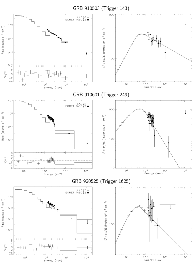
Figure 5.— Count spectra and the BEST models with sigma residuals (left panels) and corresponding $\nu F_{\nu}$ spectra (right panels) of LAD-TASC joint fits of all 15 GRBs. The BEST models are shown in solid lines in both panels. The TASC data have been binned for display purpose only.

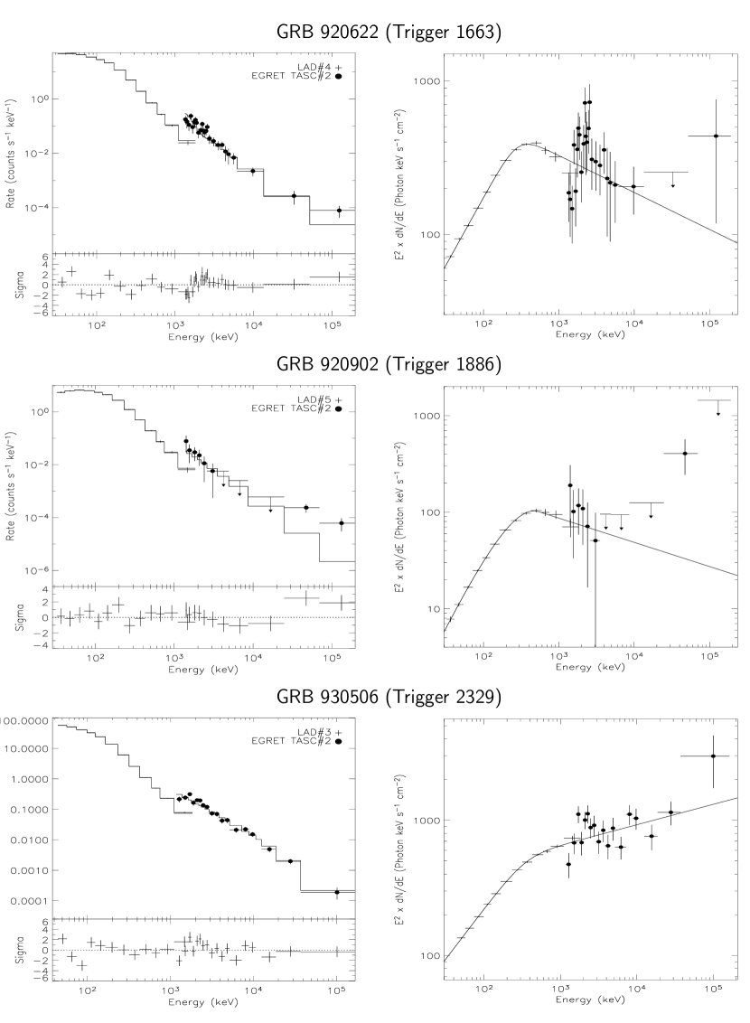
Figure 3.— Continued.

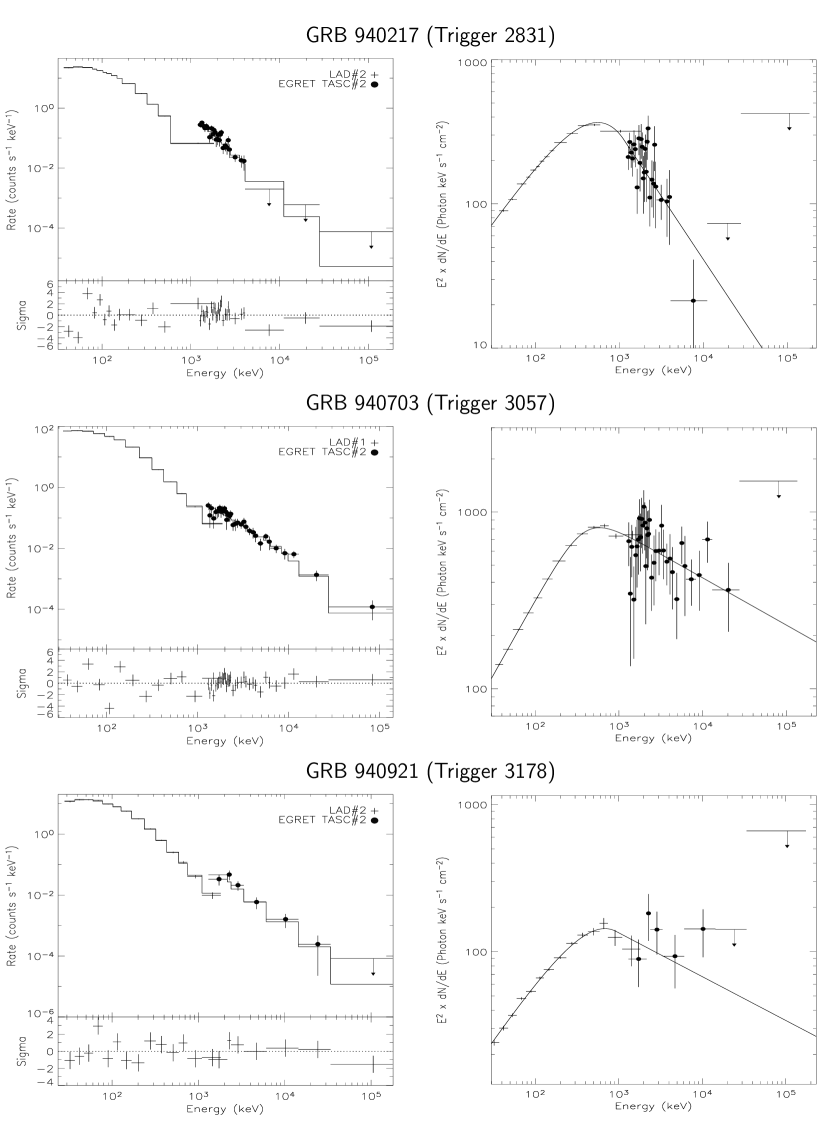
Figure 3.— Continued.

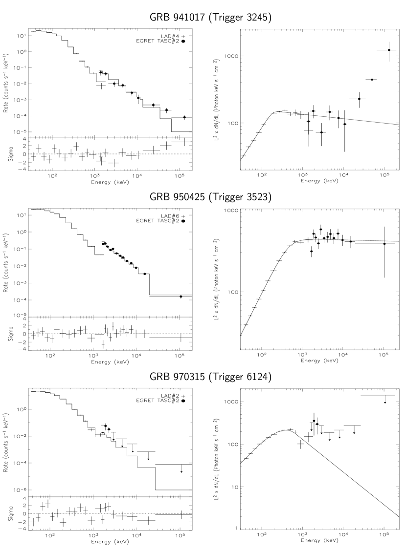
Figure 3.— Continued.

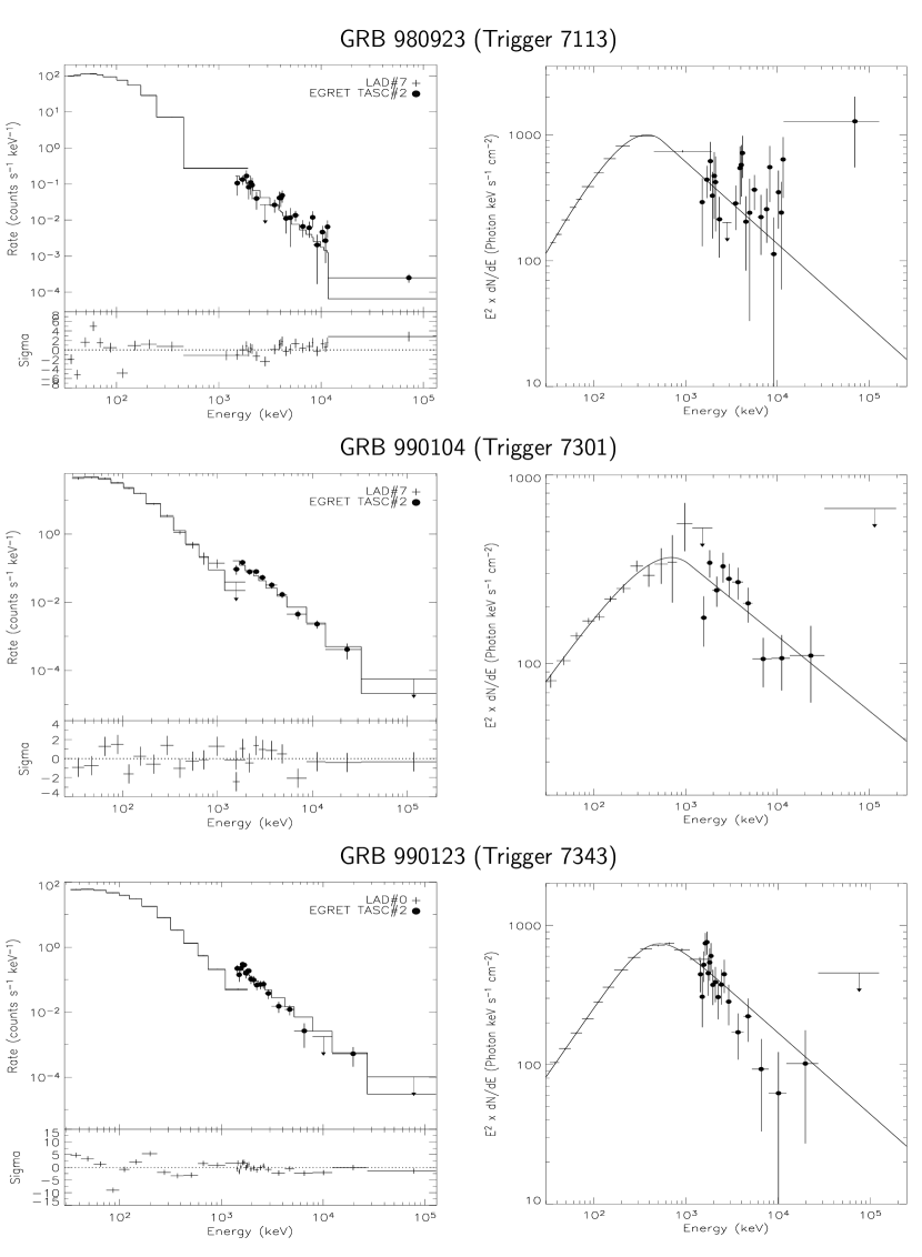
Figure 3.— Continued.

Figure 10.— Parameter distribution comparisons of 15 joint events with 342 bright BATSE GRBs. The crosses represent photon fluence (top) and spectral indices (bottom) of jointly analyzed events, and histogram shows the distribution of LAD-only analysis events.

Figure 11.— Parameter distribution comparisons of 15 joint events with 342 bright BATSE GRBs. The crosses represent ${\mathcal{E}}_{\rm pk}$ (left) and $E_{\rm b}$ (right) values of jointly analyzed events, and histogram shows the distribution of LAD events. In the ${\mathcal{E}}_{\rm pk}$ distribution, GRB 930506 (trigger 2329) is excluded due to a very high ${\mathcal{E}}_{\rm pk}$ $>167$ MeV.

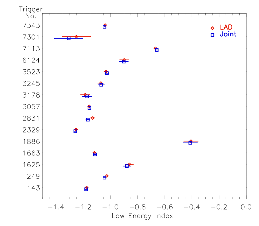
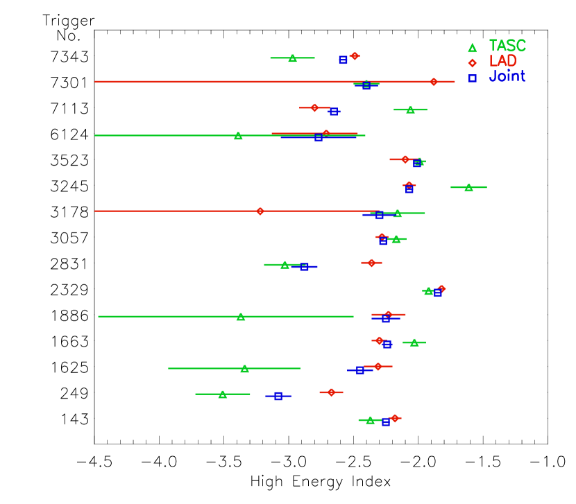
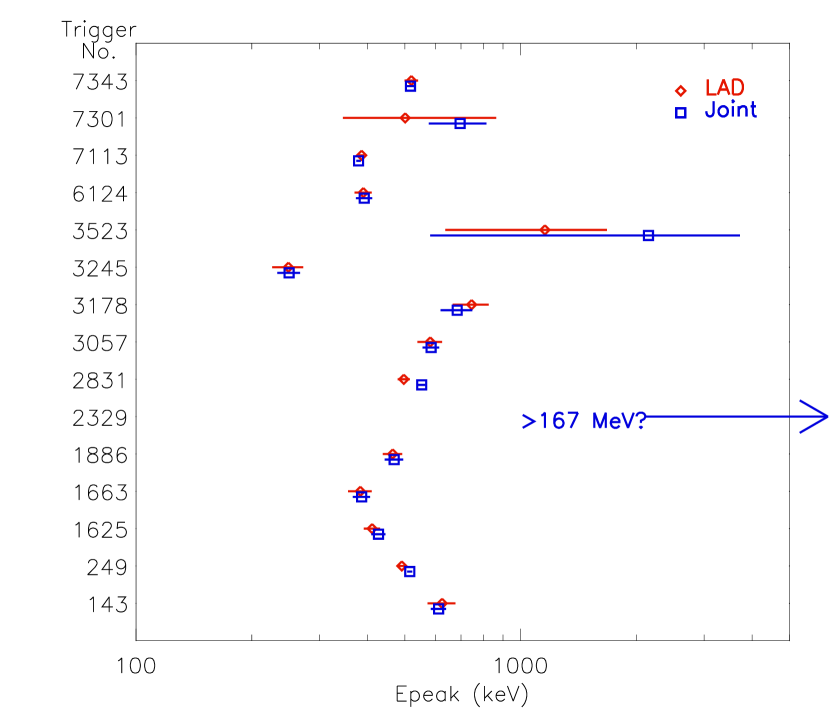
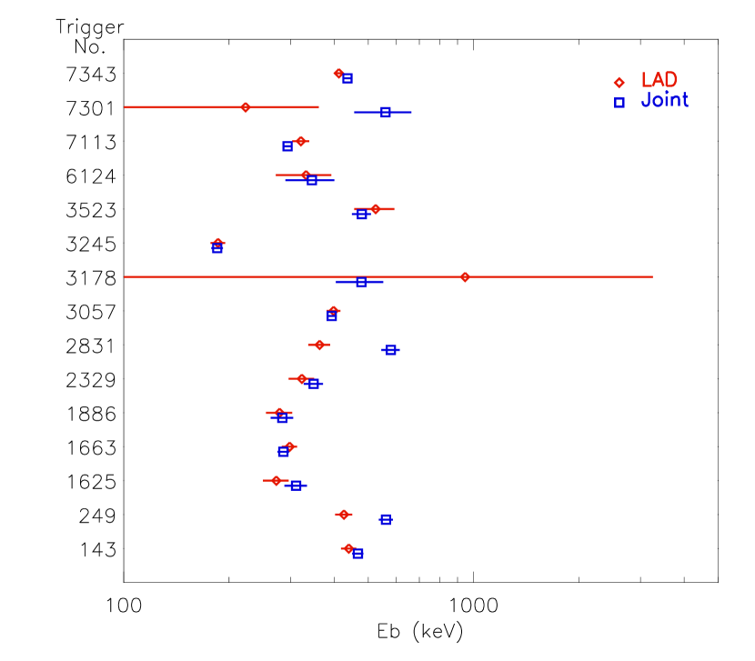
Figure 12.— Low- & high-energy indices (top panels) and ${\mathcal{E}}_{\rm pk}$ and $E_{\rm b}$ (bottom panels) determined by joint analysis (squares) and individual analysis of LAD (diamonds) and TASC (triangles). Left axis shows the event trigger numbers. All uncertainties are 1$\sigma$. ${\mathcal{E}}_{\rm pk}$ value of trigger 2329 is $>167$ MeV.

Figure 13.— Effective area correction values of 15 events as a function of their incident zenith angles. Dashed line shows the normalized TASC effective area (taken from Thompson et al., 1993), also as a function of incident zenith angle, and for azimuth angle of 168^o. Uncertainties in EAC values are 1$\sigma$.

Table 1Time and energy intervals used for the LAD–TASC joint spectral analysis of 15 GRBs. Time intervals are shown in units of second since BATSE trigger.

			Time Interval			LAD Energy			TASC Energy
GRB	BATSE	LAD	Start	End		Start	End		Start	End
Name	Trigger No.	No.	(s)	(s)		(keV)	(MeV)		(MeV)	(MeV)
910503	143	6	–9.8	88.5		36.6	1.81		1.29	201
910601	249	2	15.9	48.6		37.0	1.82		1.32	198
920525	1625	5	–18.4	47.1		32.6	1.85		1.30	195
920622	1663	4	–30.9	34.6		31.9	1.81		1.32	195
920902	1886	5	–10.2	120.8		32.7	1.85		1.39	196
930506	2329	3	–33.1	32.5		44.2	1.85		1.18	167
940217	2831	2	–8.2	188.4		37.1	1.82		1.25	187
940703	3057	1	–1.0	97.2		33.3	1.88		1.28	139
940921	3178	2	–25.6	72.6		28.1	1.82		1.31	178
941017	3245	4	–51.2	210.9		31.8	1.81		1.25	199
950425	3523	6	–23.6	107.5		36.3	1.80		1.57	197
970315	6124	2	–15.8	82.5		37.1	1.82		1.51	189
980923	7113	7	–20.0	78.7		33.4	1.92		1.44	131
990104	7301	7	–4.5	257.7		29.3	1.96		1.45	202
990123	7343	0	–0.1	98.3		33.1	1.81		1.40	128

Table 2Summary of LAD–TASC joint fit results for time-integrated spectra. Full functional form and parameter description of each spectral model can be found in K06. 1$\sigma$ uncertainties are shown in parentheses.

		Spectral Fit Parameters
GRB	BATSE	BEST	Amplitude	${\mathcal{E}}_{\rm pk}$${}^{{}^{1}}$	Low Index${}^{{}^{2}}$	High Index${}^{{}^{3}}$	$E_{\rm b}^{{}^{4}}$	Break	EAC	$\chi^{2}$/dof
Name	Trig No.	Model	(ph s-1 cm-2)	(keV)			(keV)	Scale, $\Lambda$
910503	143	SBPL	0.0116 (0.0000)	612 ( 28)	–1.18 (0.01)	–2.25 (0.03)	467 ( 17)	0.20	0.63	204.4/224
910601	249	BAND	0.0567 (0.0003)	515 (  8)	–1.04 (0.01)	–3.08 (0.10)	562 ( 26)	—	0.71	288.0/221
920525	1625	BAND	0.0151 (0.0003)	427 ( 18)	–0.88 (0.03)	–2.45 (0.10)	311 ( 23)	—	0.19	250.1/221
920622	1663	SBPL	0.0174 (0.0001)	386 ( 20)	–1.11 (0.01)	–2.24 (0.04)	286 ( 11)	0.20	0.73	228.9/220
920902	1886	BAND	0.0043 (0.0001)	469 ( 26)	–0.41 (0.05)	–2.25 (0.11)	284 ( 21)	—	0.70	110.8/219
930506	2329	SBPL	0.0220 (0.0001)	$>$167000?	–1.26 (0.01)	–1.85 (0.02)	349 ( 22)	0.30	0.50	226.6/208
940217	2831	BAND	0.0203 (0.0001)	553 ( 12)	–1.17 (0.01)	–2.88 (0.10)	580 ( 35)	—	0.49	257.7/222
940703	3057	SBPL	0.0315 (0.0001)	585 ( 29)	–1.15 (0.01)	–2.27 (0.03)	393 ( 13)	0.30	0.33	211.8/206
940921	3178	BAND	0.0067 (0.0002)	684 ( 65)	–1.17 (0.03)	–2.30 (0.13)	478 ( 74)	—	0.73	218.6/217
941017	3245	SBPL	0.0086 (0.0001)	250 ( 17)	–1.07 (0.02)	–2.07 (0.03)	185 (  7)	0.10	0.44	183.4/215
950425	3523	SBPL	0.0095 (0.0001)	2150 (1568)	–1.03 (0.02)	–2.01 (0.03)	479 ( 30)	0.30	0.69	203.8/215
970315	6124	BAND	0.0143 (0.0004)	392 ( 19)	–0.90 (0.03)	–2.77 (0.29)	345 ( 55)	—	0.63	207.3/215
980923	7113	BAND	0.0639 (0.0005)	379 (  5)	–0.66 (0.01)	–2.65 (0.05)	294 (  8)	—	0.37	267.7/198
990104	7301	BAND	0.0190 (0.0006)	696 (119)	–1.31 (0.05)	–2.40 (0.09)	560 (104)	—	0.35	202.5/217
990123	7343	SBPL	0.0256 (0.0001)	517 ( 16)	–1.04 (0.01)	–2.58 (0.03)	436 ( 10)	0.30	0.68	400.4/200

¹ Energy at which the $\nu F_{\nu}$ spectrum peaks. For BAND, it is a Fitted $E_{\rm peak}$, if $\beta<-2$, and for SBPL, it is a calculated $E_{\rm peak}$ (see Appendix B in K06).
² $\alpha$ for BAND and $\lambda_{1}$ for SBPL.
³ $\beta$ for BAND and $\lambda_{2}$ for SBPL.
⁴ Fitted $E_{\rm b}$ for SBPL, and calculated $E_{\rm b}$  for BAND (see Appendix C in K06).

References

- Band et al. (1993) Band, D.L., et al. 1993, ApJ, 413, 281
- Baring (2000) Baring, M.G., 2000, in GeV-TeV Gamma Ray Astrophysics Workshop: Towards a Major Atmospheric Cherenkov Detector VI, ed. B. Dingus, et al. AIP, 515, 238
- Briggs et al. (1999) Briggs, M.S., et al. 1999, ApJ, 524, 82
- Catelli et al. (1998) Catelli, J.R., et al. 1998, in Gamma-Ray Bursts, 4th Huntsville Symposium, ed. C. Meegan, R. Preece and T. Koshut, AIP, 428, 309
- Dermer & Atoyan (2004) Dermer, C.D. & Atoyan, A., 2004, A&A, 418, L5
- Dingus et al. (1998) Dingus, B.L., et al. 1998, in Gamma-Ray Bursts, 4th Huntsville Symposium, ed. C. Meegan, R. Preece and T. Koshut, AIP, 428, 349
- Fishman et al. (1989) Fishman, G.J., et al. 1989, in Proc. GRO Science Workshop, GSFC, 2-39
- González et al. (2003) González, M.M., et al. 2003, Nature, 424, 749
- González et al. (2004) González, M.M., et al. 2004, in Gamma-Ray Bursts: 30 Years of Discovery, ed. E. Fenimore & M. Galassi, AIP, 727, 236
- Granot & Guetta (2003) Granot, J. & Guetta, D., 2003, ApJ, 598, L11
- Guetta & Granot (2003) Guetta, D. & Granot, J., 2003, ApJ, 585, 885
- Hanlon et al. (1994) Hanlon, L., et al. 1994, A&A, 285, 161
- Harris & Share (1998) Harris, M.J. & Share, G.H., 1998, ApJ, 494, 724
- Hurley et al. (1994) Hurley, K., et al. 1994, Nature, 371, 652
- Kaneko et al. (2004) Kaneko, Y., et al. 2004, in Gamma-Ray Bursts: 30 Years of Discovery, ed. E. Fenimore & M. Galassi, AIP, 727, 244
- Kaneko et al. (2005) Kaneko, Y., et al. 2005, in Astrophysical Particle Acceleration in Geospace and Beyond, ed. D. Gallagher, et al. AGU Monograph, 156, 275
- Kaneko et al. (2006) Kaneko, Y., et al. 2006, ApJS, 166, 298 (K06)
- Katz (1994) Katz, J.I., 1994, ApJ, 432, L107
- Kippen et al. (1998) Kippen, R.M., et al. 1998, Adv. Space Res., 22, 1097
- Kwok et al. (1993) Kwok, P.W., et al. 1993, in Compton Gamma-Ray Observatory, ed. M. Friedlander, N. Gehrels & D. Macomb, AIP, 280, 855
- Mallozzi et al. (1995) Mallozzi, R.S., et al. 1995, ApJ, 454, 597
- Nelson et al. (1985) Nelson, W.R., et al. 1985, The EGS4 Code System, SLAC Rep., 265
- Paciesas et al. (1999) Paciesas, W.S., et al. 1999, ApJS, 122, 465
- Preece et al. (1994) Preece, R.D., Briggs, M.S., Mallozzi, R.S., & Brock, M.N., 1994, “WINdows Gamma SPectral ANalysis (WINGSPAN)”
- Preece et al. (2000) Preece, R.D., et al. 2000, ApJS, 126, 19
- Ryde (1999) Ryde, F., 1999, Astrophys. Lett., 39, 281
- Schaefer et al. (1998) Schaefer, B.E., et al. 1998, ApJ, 492, 696
- Schneid et al. (1992) Schneid, E.J., et al. 1992, A&AL, 255, 13
- Schneid et al. (1995) Schneid, E.J., et al. 1995, ApJ, 453, 95
- Thompson et al. (1993) Thompson, D.J., et al. 1993, ApJS, 86, 629
- Wren et al. (2002) Wren, D.N., et al. 2002, ApJ, 574, L47
- Zhang & Mészáros (2004) Zhang, B. & Mészáros, P., 2004, Int. J. Mod. Phys. A., 19, 2385