Dark Matter Halo Profiles in Scale-Free Cosmologies

Abstract

We explore the dependence of the central logarithmic slope of dark matter halo density profiles $\alpha$ on the spectral index $n$ of the linear matter power spectrum $P(k)$ using cosmological $N$-body simulations of scale-free models (i.e. $P(k)\propto k^{n}$). These simulations are based on a set of clear, reproducible and physically motivated criteria that fix the appropriate starting and stopping times for runs, and allow one to compare haloes across models with different spectral indices and mass resolutions. For each of our simulations we identify samples of well resolved haloes in dynamical equilibrium and we analyse their mass profiles. By parameterising the mass profile using a “generalised” Navarro, Frenk & White profile in which the central logarithmic slope $\alpha$ is allowed to vary while preserving the $r^{-3}$ asymptotic form at large radii, we obtain preferred central slopes for haloes in each of our models. There is a strong correlation between $\alpha$ and $n$, such that $\alpha$ becomes shallower as $n$ becomes steeper. However, if we normalise our mass profiles by $r_{-2}$, the radius at which the logarithmic slope of the density profile is $-2$, we find that these differences are no longer present. This is apparent if we plot the maximum slope $\gamma=3(1-\rho/\bar{\rho})$ as a function of $r/r_{-2}$ – we find that the profiles are similar for haloes forming in different $n$ models. This reflects the importance of concentration, and reveals that the concentrations of haloes forming in steep-$n$ cosmologies tend to be smaller than those of haloes forming in shallow-$n$ cosmologies. We conclude that there is no evidence for convergence to a unique central asymptotic slope, at least on the scales that we can resolve.

1 Introduction

The currently favoured model of cosmological structure formation asserts that the Universe is dominated by some form of non-baryonic Cold Dark Matter (hereafter CDM), and it makes a number of generic predictions about how the dark matter clusters on small scales. Arguably the defining prediction of the CDM model is that the radial mass density profile of dark matter haloes is divergent at small radii, which leads to a central density “cusp”. Characterising the form of this mass density profile has been one of the most active research problems in computational cosmology over the last decade.

The seminal study of Navarro, Frenk & White (1996,1997; hereafter NFW) introduced the concept of a “universal” mass density profile for dark matter haloes that form in hierarchical clustering cosmologies. This NFW profile is written as

$$\rho(r)=\frac{\rho_{c}}{\left(r/r_{s}\right)(1+r/r_{s})^{2}}\ ,$$ (1)

where $r_{s}$ is a scale radius and $\rho_{c}$ is a characteristic density, which can be related to $r_{s}$ once the virial mass of the halo is fixed; equation 1 describes a one-parameter family of curves. It is convenient to rewrite equation 1 in the more general form

$$\rho(r)=\frac{\rho_{c}}{\left(r/r_{s}\right)^{\alpha}(1+r/r_{s})^{3-\alpha}}\ ,$$ (2)

where $\alpha$ is the central asymptotic logarithmic slope. The NFW profile is “universal” in the sense that it describes the ensemble averaged mass profile of dark matter haloes in dynamical equilibrium, independent of virial mass, cosmological parameters and initial power spectrum.

During the last decade numerous studies have investigated whether or not the NFW profile does indeed provide an adequate description of the mass profile of dark matter haloes, and to understand the physical mechanisms that shape the functional form of the profile. NFW recognised that $r_{s}$ correlates with the virial mass of the halo, increasing with decreasing virial mass. They argued that this virial mass–scale radius relation is an imprint of the hierarchical assembly of haloes; low-mass haloes tend to collapse before high-mass haloes, when the mean density of the Universe is higher, and $r_{s}$ reflects the mean density of the Universe at the time of collapse.

The halo sample that formed the basis of Navarro et al. (1997) contained of order $10^{4}$ particles (and hence resolving the profile down to about 10% of the virial radius, according to the convergence criteria of Power et al. (2003)). Subsequent studies drew upon haloes containing about two orders of magnitude more particles within the virial radius and confirmed the basic finding of NFW that CDM haloes are cuspy (e.g. Fukushige & Makino 1997; Moore et al. 1998; Jing & Suto 2000; Jing 2000; Fukushige & Makino 2001; Jing & Suto 2002). These studies led to debate about the exact value of the logarithmic inner slope, which ranged from $\alpha\sim 1$ to $1.5$ (e.g., Navarro et al. 1997, Moore et al. 1999). The study of Power et al. (2003) provided convergence criteria that allowed simulators to understand the impact of numerical artifacts on the central structure of haloes, and to identify the innermost radius at which the mass profile could be considered reliably resolved. More recently, a great deal of effort has gone into even higher resolution simulations that have revealed density profiles of CDM haloes to well within $1\%$ of the virial radius (Fukushige et al. 2004; Tasitsiomi et al. 2004; Navarro et al. 2004; Reed et al. 2005; Diemand et al. 2005). The highest resolved simulation to-date reached an effective mass resolution of about 130 million particles in a cluster sized dark matter halo still supporting the evidence for a central cusp with a logarithmic inner slope of about $\alpha\sim 1.2$ (Diemand et al., 2005).

Cosmological simulations allow us to characterise the functional form of the density profile and to explore the important physical processes (e.g. merging, smooth accretion) that drive this form (cf., Lu et al., 2006; Salvador-Solé et al., 2007), but a theoretical understanding of the origin of the mass profile is essential. Is the form of the profile set by non-linear processes during the virialisation of the halo, or is there an imprint of the primordial power spectrum $P(k)$?

One must make strong assumptions about the connection between density and velocity dispersion to obtain analytical predictions about halo structure. For example, under the assumption that the phase-space density is a power law in radius as suggested by Taylor & Navarro (2001) one can solve the spherical Jeans equation to obtain the density profile (Hansen 2004; Dehnen & McLaughlin 2005; Austin et al. 2005). These studies, guided by the results of the numerical simulations, confirm the central logarithmic slope to be in the range $\alpha\sim 1$ to $2$, although Hansen & Stadel (2006) have claimed that equilibrated haloes have central slopes of $\alpha\sim 0.8$.

However, it is interesting to ask whether or not there is a dependence of halo structure on the primordial power spectrum $P(k)$. In particular, does the form of the profile depend on the (effective) spectral index $n$ of $P(k)$? One of the key predictions of the NFW papers is that the shape of the “universal” profile should hold in any hierarchical cosmology, including scale-free ones. This was confirmed by subsequent numerical simulations (e.g. Cole & Lacey, 1996). However, a number of analytical studies have claimed that the density profile should depend on spectral index (e.g., Hoffman & Shaham, 1985; Syer & White, 1998; Subramanian et al., 2000; Huffenberger & Seljak, 2003; Salvador-Solé et al., 2007), and these have been supported by numerical simulations providing similar evidence (e.g., Crone et al., 1994; Eke et al., 2001; Ricotti, 2003; Cen et al., 2004; Reed et al., 2005; Ricotti et al., 2007).

Within this context it is interesting to consider the findings of Ricotti (2003) and Cen et al. (2004). Both studies analysed high-resolution cosmological simulations and each argued that dark matter haloes at high redshifts have shallow central logarithmic slopes, with $\alpha\approx 0.2-0.4$. In particular, Ricotti (2003) claimed that the central logarithmic slope depends explicitly on the effective spectral index $n$, in agreement with the predictions of Subramanian et al. (2000). We note that Colín et al. (2004) performed and analysed simulations comparable to those presented in Ricotti (2003) and found no evidence for the shallow “cores” ($\alpha\sim 0.2$); rather they found that their data favoured “cusps” ($\alpha\approx 1$). However, Ricotti et al. (2007) have recently revisited this topic using simulations with higher mass and force resolution, and they continue to argue in favour of shallow cores, in agreement with their earlier study.

Ricotti (2003) and Ricotti et al. (2007) sought to isolate the effect of spectral index $n$ on halo structure by using a series of simulations of the $\Lambda$CDM model with different box-sizes and evolved for different numbers of expansion factors, to mimic a single $n$. In this short paper we revisit this topic and the claims of Ricotti (2003) and Ricotti et al. (2007) using high resolution cosmological $N$-body simulations of scale-free models in which we vary systematically the spectral index $n$. This “clean” approach allows us to study whether the density profiles of dark matter haloes indeed show a dependence on the spectral index $n$.

In § 2 we give a detailed description of how we have set up and run our scale-free simulations. There are some important issues to be considered when deciding on when to start a scale-free simulation and when to stop the simulation to compare halo properties. We encapsulate our findings in a set of well defined and physically motivated criteria. In § 3 we present the results of our analysis of the halo mass profiles, and we summarise our results in § 4.

2 Numerical simulations

As we intend to perform scale-free cosmological simulations, we use a power law for the initial power spectrum of the simulation

$$P\left(k\right)=a^{2}AP_{\mathrm{WN}}\left(\frac{k}{k_{\mathrm{Ny}}}\right)^{n},$$ (3)

with $A$ being the amplitude scaling factor and

$$P_{\mathrm{WN}}=\left(\frac{L}{N}\right)^{3}\quad\mathrm{and}\quad k_{\mathrm{Ny}}=\frac{N\pi}{L}$$

denoting the power of the white noise of a random distribution of $N^{3}$ particles in a box with size $L$ and the Nyquist frequency, respectively. The simple scaling with expansion factor $a$ is valid only for an Einstein–de Sitter universe, which is the cosmology of our choice. The box-size $L$ is completely arbitrary because of the scale-free nature of the power spectra, and so we set it to $1$ Mpc. $N$ denotes the number of particles along one dimension. We run a sequence of simulations with the parallel $N$-body code Gadget2 (Springel, 2005) containing $512^{3}$ particles that differ only in the value of the spectral index $n$; we use $n$=-0.50, -1.50, -2.25, -2.50 and -2.75.

In order to set-up and run the simulations, we still need to specify the amplitude scaling factor $A$ for all models and to find a criterion for when to stop and compare objects from different runs. These two choices will be presented and discussed in the following two subsections.

2.1 Initial Conditions

For setting up the initial conditions of the simulations, only the amplitude scaling factor $A$ in equation 3 needs to be determined; all other factors are given by the specifics of the model under investigation, i.e. $N$ and $n$. The mass fluctuations $\sigma^{2}_{\mathrm{box}}$ within the computational domain can be written as follows

$$\sigma^{2}_{\mathrm{box}}=\left(\frac{1}{2\pi}\right)^{3}\int_{\mathrm{box}}\mathrm{d}\mn@boldsymbol{k}\,P\left(k\right)$$ (4)

where the integration range in $\mn@boldsymbol{k}$ contains all significant frequencies reproduced in the box, e.g.. $k_{x,y,z}\in\left[2\pi/L,N\pi/L\right]$. With the definition of $P(k)$ (cf. eq. 3) this can be evaluated analytically to be

$$A=\frac{2\pi^{2}\sigma^{2}_{\mathrm{box}}}{k_{\mathrm{Ny}}^{3}P_{\mathrm{WN}}}\frac{n+3}{1-\left(\frac{\sqrt{2}}{N}\right)^{n+3}}.$$ (5)

Here we use $\sqrt{2}$ rather than $\sqrt{3}$ in the denominator because surface diagonals occur more frequently than volume diagonals. Hence by specifying $\sigma_{\mathrm{box}}$ we also fix the amplitude scaling factor $A$. For our simulations we choose $\sigma_{\mathrm{box}}$ to be $0.15$ and therefore start all models with the same “integral power”, independent of spectral index $n$.

This choice for the normalisation of the initial power spectrum deviates from the usual course of action to fix the power at the Nyquist frequency $k_{\mathrm{Ny}}$ at the white noise level. Our experience tells us that such runs start at too late a stage, especially for $P(k)$ with a rather steep $n$, because the mass variance $\sigma_{\rm box}$ can be large and possibly non-linear. We note that previous studies have arbitrarily lowered the amplitude to $1/4$ of the white noise level for such models to circumvent this problem (Efstathiou et al. 1988; Lacey & Cole 1994; Navarro et al. 1997).

Table 1 lists the amplitudes derived from equation 5 in terms of the white noise level $P_{\mathrm{WN}}$. Figure 1 verifies that we recover the input power spectra from our initial conditions for the selection of the models under investigation.

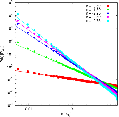
Figure 1: Shown are the theoretical power spectra and their respective realisations in the initial conditions of the simulations we performed.

2.2 Stopping Criterion

In order to define an end-point for our scale-free simulation that allows for a cross-comparison of identified haloes amongst runs with different $n$ values we follow Navarro et al. (1997) and track the evolution of $M_{*}(a)$, the typical collapsing mass of an object in our simulation at expansion factor $a$. This “non-linear” mass scale is defined by requiring that the variance of the linear overdensity field, smoothed with a top-hat filter enclosing a mass $M=M_{*}(a)$, should equal the square of the critical density threshold for spherical collapse (e.g., Press & Schechter 1974, Navarro et al. 1997)

$$\sigma^{2}_{M_{*}}=\delta^{2}_{\mathrm{crit}}.$$ (6)

The mass variance $\sigma^{2}_{M}$ is related to the matter power spectrum $P(k)$ via

$$\sigma_{M}^{2}=\frac{1}{2\pi^{2}}\int_{0}^{+\infty}P(k)\hat{W}^{2}(kR)k^{2}dk,$$ (7)

where $\hat{W}(x)=\frac{3}{x^{3}}(\sin{x}-x\cos{x})$ is the Fourier-transform of the top-hat window function, and $R=\left(3M/4\pi\rho_{\mathrm{crit}}\right)^{1/3}$ relates the spatial scale to a mass scale.

$M_{*}(a)$ is a monotonic function of the cosmic expansion factor $a$ and has a different shape depending on the choice of the spectral index $n$. We still need to select a fiducial value $M_{*,\mathrm{f}}$ (independent of $n$) defining $a_{\rm f}(n)$ via inverting $M_{*,\mathrm{f}}=M_{*}\left(a_{\rm f}(n)\right)$ for each of our scale-free models. A careful investigation of the maximal allowed expansion factor in the $n=-2.5$ model leaves us with $M_{*,\mathrm{f}}\approx 42000$ particles (please refer to Appendix A for more details). The adopted $a_{\rm f}(n)$ values are listed in Table 1.

Table 1: The parameters for the initial conditions for the simulations.

model	$n$	$A$	$a_{\mathrm{f}}$
512-0.50	$-0.50$	$0.0358$	$826.0$
512-1.50	$-1.50$	$0.0215$	$161.5$
512-2.25	$-2.25$	$0.0109$	$43.9$
512-2.50	$-2.50$	$0.0076$	$27.3$
512-2.75	$-2.75$	$0.0046$	$16.7$

$A$ is the amplitude and $n$ the slope of the initial power spectrum. The quantity $a_{\mathrm{f}}$ gives the adopted expansion of the universes that will lead to about 42000 particles in an $M_{*}$ halo.

3 Analysis

In this section we first discuss the tool employed to identify haloes (section 3.1) and the selection criteria used to define the sample of virialised haloes (section 3.2). We then employ two approaches to characterise halo structure – a straightforward parameter fit to the density profile to assess the dependence of $\alpha$ on $n$ (section 3.3), and a non-parametric estimate of central concentration of the halo based on $r_{-2}$, the radius at which the logarithmic slope of the density profile is $-2$ (section 3.4). These measures of the mass profile allow us to explore the dependence of inner slope on the spectral index.

3.1 Halo identification

We used an MPI version of the AMIGA Halo Finder (AHF, successor of MHF introduced in Gill et al. (2004)) for identifying haloes and computing their integral and radial properties. AHF locates haloes as peaks in an adaptively smoothed density field using a hierarchy of grids and a refinement criterion that is comparable to the force resolution of the simulation (i.e. 5 particles per cell). Local potential minima are calculated for each of these peaks and the set of particles that are gravitationally bound to the peaks are identified as the groups that form our halo catalogue. Each halo in the catalogue is then processed, producing a range of structural and kinematic information. Haloes are defined such that the virial mass is $M_{\rm vir}=4\pi\rho_{\rm crit}\Delta_{\rm vir}r_{\rm vir}^{3}/3$, where the overdensity criterion $\Delta_{\rm vir}=178$ for an Einstein-de Sitter cosmology.

3.2 Halo selection

We restrict our analysis to only those haloes that contain in excess of $3.15\times 10^{4}$ particles($\simeq 0.75M_{*}$) within the virial radius. Furthermore we employ a criterion to exclude objects that we do not expect to be in dynamical equilibrium. For this we use $\Delta_{r}$, the displacement of the centre of mass of all material within the virial radius with respect to the centre of potential of the halo, normalised to the virial radius of the halo;

$$\Delta_{r}=\frac{|\vec{r}_{\rm cm}-\vec{r}_{\rm cen}|}{r_{\rm vir}}$$ (8)

We reject all haloes for which $\Delta_{r}>0.05$. This is a more conservative requirement than has been used in other recent studies (e.g. Neto et al., 2007). However, we show in another paper (Power et al, in prep.) that this ensures that a halo is unlikely to have experienced a merger with mass ratio greater than 10% in the previous dynamical time (defined at the virial radius).

Additionally we define a subset of the catalog, consisting of haloes at about $M_{*}$: we use objects in the mass range of $0.75M_{*}$ to $1.5M_{*}$ which corresponds to halos with a number of particles $N\in[3.15,6.30]\times 10^{4}$. In table 2 we give a summary of the number of haloes used in our analysis.

Table 2: Definition of various halo samples.

Run	all	$M_{*}$ sample	high-mass sample
512-0.50	276	186	38
512-1.50	172	107	44
512-2.25	119	62	33
512-2.50	64	35	19
512-2.75	38	15	16

The columns give the number of haloes that satisfy our selection criteria. The first column gives the total number of objects consisting of more than $3.15\times 10^{4}$ particles; we refer to it as “all”. The second column gives the number of objects in our $M_{*}$ sample, i.e. haloes with masses in the range $M\in[0.75,1.5]M_{*}$. Finally we list the number of haloes with more than $N>10^{5}$ particles, which we refer to as “high-mass sample”. Note that all haloes satisfy our the centre-of-mass offset criterion and are therefore considered to be in dynamical equilibrium.

3.3 The Preferred Slope $\alpha$

We begin our study of the dependence of the central logarithmic slope $\alpha$ on the spectral index $n$ by fitting the generalised NFW profile (cf. equation 2) to each halo in our $M_{*}$ sample. Recall that

$$\rho\left(r\right)=\frac{\rho_{c}}{\left(\frac{r}{r_{s}}\right)^{\alpha}\left(1+\frac{r}{r_{s}}\right)^{3-\alpha}}$$ (9)

where $r_{s}$ and $\rho_{c}$ are the fitted parameters. We perform several fits for each profile, varying $\alpha$ in the range of $\alpha=0.3,\dots,1.8$. The case of $\alpha=1.0$ corresponds to the NFW profile.

For each halo we determine a set of parameters for each choice of $\alpha$. By comparing the $\chi^{2}$-value we can, in principle, find the preferred $\alpha$ for a halo. However, we are interested in whether or not $\alpha$ depends on $n$ for a typical halo, and so a statistical analysis is required. Therefore, we define a quality measure of the fit,

$$Q_{j}=\frac{\sum_{\mathrm{bins}}\left(\frac{X_{ij}-\rho_{\mathrm{fit}}\left(r_{i}\right)}{X_{ij}}\right)^{2}}{\mathrm{dof}};$$ (10)

here $\mathrm{dof}$ denotes the number of degrees of freedom of the fit, $X_{ij}$ the density value of the $j$th halo in the $i$th radial bin and $\rho_{\mathrm{fit}}$ the corresponding value of the analytic function at radius $r_{i}$.

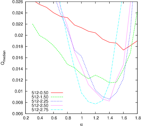
Figure 2: The median of the quality in the different simulation boxes for objects in the $M_{*}$ sample.

Taking the median $Q$ in each simulation box for each value of $\alpha$ we can explore how the preferred inner slope of the density profile depends on the spectral index $n$, as shown in Figure 2. Each curve indicates how the quality of the fit varies with $\alpha$ for a given $n$, and the minima of the curves pick out the preferred $\alpha$ for a particular $n$. For the $n=-0.5$ run we find a minimum at $\alpha\simeq 1.6$, while for the $n=-2.75$, the preferred $\alpha\simeq 1.2$. Even though the curves for the $n=-1.5$ ($-2.25$, $-2.5$) runs seem to have their minima at $\alpha\simeq 1.4$, a trend can be seen. Therefore we might conclude that the preferred $\alpha$ decreases with decreasing $n$; that is, the steeper the spectral index, the shallower the central logarithmic slope.

However, care must be taken when interpreting slopes. Close inspection of equation 9 will reveal that the logarithmic slope will depend on the scale radius $r_{s}$. Therefore, an apparent trend in $\alpha$ with $n$ may instead be attributable to a trend in $r_{s}$ with $n$. If $r_{s}$ is systematically smaller in a model with spectral index $n_{1}$ when compared to a model with spectral index $n_{2}$, haloes will be systematically more concentrated and so fits to the resolved part of the density profile will produce higher “effective” slopes $\alpha$. We investigate this further in § 3.4.

3.4 The Maximum Slope $\gamma$

A useful non-parametric measure of halo structure is the maximum asymptotic slope,

$$\gamma\left(r\right)=3\left(1-\frac{\rho(r)}{\bar{\rho}(r)}\right),$$ (11)

which uses the local mass density $\rho$ and the enclosed mass density $\bar{\rho}$ to derive an upper limit to the logarithmic slope of the density profile at radius $r$. Equation 11 assumes that the halo is spherically symmetric with a density profile interior to $r$ given by a power-law, $\rho(r)\propto r^{-\gamma}$. $\gamma$ defines an upper limit to the slope; a steeper slope would require more mass interior to $r$ than is measured. We note that this measure was used by Navarro et al. (2004) for resimulated haloes of different masses but comparable particle resolution in their study of the universality of the mass profile.

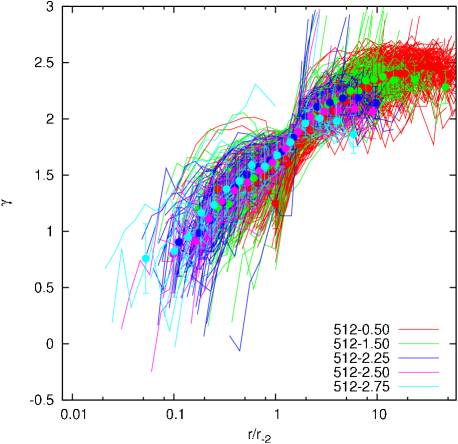
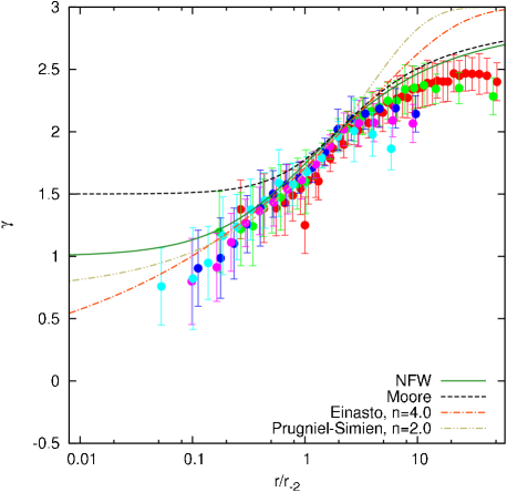
Figure 3: The maximal inner slope as given by equation 11 as a function of the radius normalised to $r_{-2}$ for haloes in the $M_{*}$ sample. Upper panel: We plot all curves from all the simulations and over-plot a binned curve for each run. Lower panel: Here only the averages of each simulation are shown and compared to a set of theoretical predictions derived from the NFW, Moore et al., Einasto and Prugniel-Simien profiles. Note that in this instance $n$ corresponds to the shape parameter for the Einasto and Prugniel-Simien profiles.

In Figure 3 we plot the radial variation of $\gamma$ for all haloes that satisfy the selection criteria of § 3.2 and are in the same mass-range as those used in section 3.3, colour-coded according to the spectral index $n$ of the model in which they form. Note that we have normalised these profiles to $r_{-2}$, the radius at which the differential mass profile $\rho\,r^{2}$ reaches a maximum. For a NFW profile, $r_{-2}$ is identical to the scale radius $r_{s}$ and so it provides an attractive non-parametric measure of concentration.

When normalising the radius in this manner, we find excellent agreement between the average shapes of the $\gamma$ profiles between the different $n$ models. However, the scatter between profiles within a given simulation is significant (cf. upper panel of figure 3), which strengthens our argument that it is essential to use a statistical sample of haloes when discussing the asymptotic inner slope. It is noticeable that the average profile in each model we have looked at continues to becomes shallower with decreasing radius, without showing evidence for convergence to an asymptotic value (c.f. Navarro et al., 2004). We find similar behaviour when considering only haloes in the high-mass sample.

This figure also confirms our suspicion that it is the scale radius $r_{-2}$ or concentration $c_{\rm vir}=r_{\rm vir}/r_{-2}$ rather than the slope $\alpha$ that varies with $n$. We find that haloes forming in the $n=-0.5$ model tend to be more concentrated (cf. figure 4 below) than haloes forming in runs with steeper spectral indices. Therefore fits with a generalised NFW profile (cf. equation 9) tend to favour smaller values of $\alpha$ for steeper $n$ because these haloes tend to be less concentrated, and so we resolve the profile to smaller fractions of $r_{-2}$, where the flattening of the profile is more apparent. Therefore a shallower effective slope $\alpha$ will tend to be preferred.

It is a relatively straightforward exercise to obtain expressions for equation 11 for the NFW profile and the Moore et al. (1998) profile. Two other analytical model profiles have been promisingly applied to halo density profiles, the Einasto (1965) and Prugniel & Simien (1997) profiles, which provide better fits than the NFW profile. Merritt et al. (2006) argue that the Einasto model performed best in fitting halo profiles, followed closely by the Prugniel-Simien model. Expressions for $\gamma$ for the Einasto and Prugniel-Simien models are given in the Appendix B.

In the lower panel of figure 3 we over-plot the averaged $\gamma$-curves with the theoretical predictions derived for the four analytic profiles mentioned above. We find that the Moore profile is unable to reproduce the observed behaviour. The NFW profile is consistent with our data for the 512-0.50 and 512-1.50 runs, but it fails to reproduce the continual flattening of $\gamma$ to small radii. In contrast, both the Einasto and Prugniel-Simien profiles capture the behaviour of our data well at small radii. Interestingly we note that all of the analytical profiles tend to overestimate the slope of the density profile at large $r/r_{-2}$, which appears to roll over and flatten off. This is most apparent for the data points from the $n=-0.5$ run.

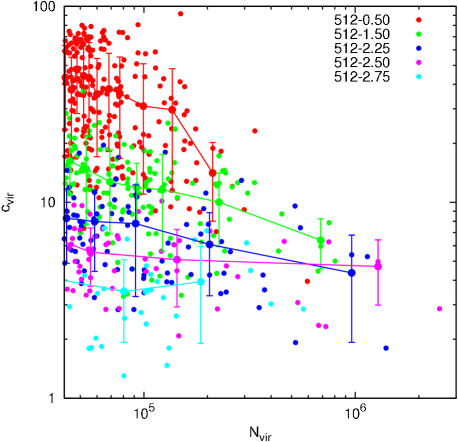
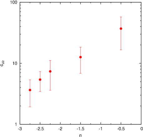
Figure 4: In the upper panel we show the concentration of all haloes with mass larger than $M_{*}$ as a function of the number of particles within the virial radius. Additionally we plot a binned distribution of the concentration. The lower panel gives the mean concentration for objects in our $M_{*}$ sample depending on the spectral index $n$.

In Figure 4 we make explicit the connection between $r_{-2}$ and the concentration $c_{\rm vir}=r_{\rm vir}/r_{-2}$, showing how $c_{\rm vir}$ varies with halo mass (given by the number of particles within the virial radius $N_{\rm vir}$; upper panel), and the spectral index $n$ (lower panel). A similar figure can be found in Navarro et al. (1997), who looked at scale-free models with spectral indices of $n=-0.5,-1.0,-1.5$, but who derived their concentrations from fits of NFW profiles. Although our concentrations are calculated in a non-parametric manner, it is reassuring that we see a similar trend to that reported in  Navarro et al. (1997). The variation of concentration with mass (upper panel) suggests that this relation may be steeper in cosmologies with shallower spectral indices, which in turn may reflect the importance of merging for the growth of the most massive haloes in these cosmologies. Although the trends are tentative, we believe that this is an extremely interesting figure and one that may allow to better understand the physical origin of the density profile. We shall return to this issue, albeit briefly, in § 4.

The trend for concentration to decrease with steeper spectral index is more robust, and we show this explicitly by plotting the mean concentration of haloes in the $M_{*}$ sample versus spectral index (lower panel). This makes clear our assertion that it is the concentration that depends strongly on the spectral index.

4 Summary & Conclusions

The primary motivation for this paper has been to establish what dependence, if any, the logarithmic slope $\alpha$ of the inner mass density profile of dark matter haloes has on the spectral index $n$ of the linear matter power spectrum. For this purpose we have run a series of high resolution cosmological $N$-body simulations of scale-free models (i.e. $P(k)\sim Ak^{n}$) with values of the spectral index $n$ varying between $-0.5\geqslant n\geqslant-2.75$. By using scale-free models and fixing $n$ in this manner, the problem of identifying correlations between $\alpha$ and $n$ becomes a relatively straightforward one. Relatively, because there is some freedom in the choice of criteria one can use to determine when to start and when to finish scale-free simulations.

To address this, we have derived clear, reproducible and physically motivated criterion that allows us to set up scale-free simulations and that is presented in § 2.1. In short, we start the simulations with the same integral power in the $k$-range defined by the the total number of particles $N$; it is especially important to have an objective criterion for starting simulations when studying mass profiles. To determine when to stop our simulations, we follow Navarro et al. (1997) and use the evolution of the typical collapsing mass $M_{*}$. We do so once the mass in a typical $M_{*}$ halo corresponds to approximately $42000$ particles.

Having established a set of well-defined criteria to set up and run cosmological simulations of scale-free models, we performed a sequence of high resolution runs ($1h^{-1}\rm Mpc$ boxes, $512^{3}$ particles) that we used to investigate the dependence of the central logarithmic slope of the dark matter halo density profile $\alpha$ on the spectral index $n$. We varied $n$ between $-0.5$ and $-2.75$ and selected samples of well resolved haloes ($N_{\rm vir}\geqslant 3.15\times 10^{4}$) in dynamical equilibrium in each run (ranging from $\sim 270$ haloes in the $n=-0.5$ run to $\sim 40$ haloes in the $n=-2.75$ run). Using $\chi^{2}$ fits to a generalised NFW profile, we identified preferred values of the inner slope $\alpha$ and indeed, we found a trend for the inner slope to become shallower with steeper spectral index – from $\alpha\simeq 1.6$ for $n=-0.5$ to $\alpha\simeq 1.2$ for $n=-2.75$.

However, we argue that it is not the central slope $\alpha$ that depends on spectral index; rather, it is the scale radius of the halo, $r_{s}$, or our preferred measure $r_{-2}$, the radius at which the differential mass profile $\rho\,r^{2}$ reaches its maximum value. We have shown that haloes in different $n$ models have similar radial profiles of the maximum slope $\gamma=3(1-\rho/\bar{\rho})$ when normalised to $r_{-2}$. However, as already shown by Navarro et al. (1997), haloes that form in models with steeper $n$ tend to be less centrally concentrated than haloes forming in models with shallower $n$, and so their mass profiles can be resolved to smaller fractions of $r_{-2}$, where the flattening of the profile is more apparent. Haloes in these models would then appear to have shallower central profiles.

We noted in the introduction that using scale-free simulations to study the effect of the spectral index of the power spectrum on the central structure of dark matter haloes was preferable to the approach taken by Ricotti (2003), Cen et al. (2004), Colín et al. (2004), and Ricotti et al. (2007), in which the box size and analysis redshift were varied to capture the behaviour of different spectral indices. The claims of Ricotti et al. (2007) are of particular interest; these authors argue that halo concentration is a universal constant and that dwarf galaxies identified at $z$=10 have logarithmic slopes shallower than $0.5$.

Our results strongly disagree with these claims. Although the central slope $\alpha$ that we obtain by fitting a generalised NFW profile does vary with $n$, this does not imply that the shape of the profile is sensitive to $n$, for the reasons presented above. Moreover, as we show in Figure 3, density profiles normalised by $r_{-2}$, which is equivalent to concentration, have similar shapes on average, independent of spectral index; this implies that it is $r_{-2}$ and consequently concentration that depends on $n$. It is possible that our profiles for $\gamma(r)$ may roll over and approach different asymptotic value at smaller radii than we can resolve with our simulations, but over the range of radii that we can reliably resolve we find no evidence for such behaviour. It should be noted that we checked for this by producing figure 3 for haloes in the high-mass sample (cf. Table 2) but we did not find any evidence for convergence.

We briefly consider the dependence of $r_{-2}$ on $n$. We show in figure 4 that haloes forming in cosmologies with steeper spectral indices tend to be less centrally concentrated than haloes forming in cosmologies with shallower spectral indices, confirming and extending results presented by Navarro et al. (1997). This is interesting because we expect that haloes forming in shallow-$n$ models do so predominantly by accretion, whereas haloes in steep-$n$ models form via merging. If we examine the mass concentration relation in shallow-$n$ models (upper panel in figure 4), we find that more massive haloes tend to be less centrally concentrated than their less massive counterparts. In contrast, we find that this relation is far less pronounced in steep-$n$ models.

Prescriptions for halo concentration, such as Eke et al. (2001), assert that concentration is determined by the halo’s collapse redshift – haloes that collapse earlier do so when the mean density of the Universe is higher, and so they tend to be more centrally concentrated. It has been argued that this reflects the rate at which the proto-halo accretes mass (cf. Zhao et al., 2003). Haloes are said to assemble their mass in two distinct phases – fast-accretion phase during which the depth of the potential well is set, and a slow-accretion phase during which mass is added to the outer parts of the halo (e.g Lu et al., 2006). This has important implications for the concentration. For example, Wechsler et al. (2002) argued that during the fast accretion phase the central density is set by the background density, but as the accretion rate slows and the halo enters its slow accretion phase, the central density stays approximately constant and the halo’s concentration grows in step with the virial radius. Merging also plays an important role; for example, Manrique et al. (2003) looked at the effect of major mergers on concentration and found that violent relaxation drives the remnant’s density profile towards a form that is essentially identical to the one it would have formed through pure accretion.

What can we learn about the physical origin of the density profile from our simulations? As we noted above, haloes in shallow-$n$ models grow predominantly by accretion, whereas those in steep-$n$ models grow via merging. This link between spectral index and accretion rate can be made explicit (see, for example, Lu et al., 2006), which makes the scale-free simulation a very interesting tool with which to study the origin of the profile. The results – that concentrations tend to be higher in shallow-$n$ models, and that concentration decreases with increasing virial mass in these models (assuming that merging plays a role in the growth of the most massive halos) – indicate that “two-phase accretion” may be very important. However, to properly address this question a more detailed study is required. We are currently undertaking such a study, an account of which will be presented in a future paper.

Appendix A Maximal Expansion

A natural stopping criterion for a scale-free cosmological simulation is given by the requirement that the fundamental mode (or a multiple of it) turns non-linear; this defines a maximal expansion $a_{\mathrm{max}}$ (cf. Efstathiou et al., 1988). But we like to remind the reader that in this study we compared simulations run with varying $n$ values and hence had to define a different stopping criterion that allows us to cross-compare those runs at a similar evolutionary stage.

However, in order to determine the maximal allowed expansion to obtain the fiducal $M_{*,\mathrm{f}}$ value we follow Efstathiou et al. (1988) and define a critical wavenumber $k_{0}$, corresponding to a filtering scale for which the rms density fluctuations approach unity

$$\left<\sigma^{2}\right>_{k_{0}}=\left(\frac{1}{2\pi}\right)^{3}\int_{\mathbb{R}^{3}}\mathrm{d}\mn@boldsymbol{k}\,P\left(k\right)\mathrm{e}^{-\left(k/k_{0}\right)^{2}}=1.$$ (12)

This equation divides the power spectrum in two parts: for all frequencies below the critical frequency $k_{0}$ the growth is still linear and for all higher frequencies the growth is non-linear. Solving equation 12 for $k_{0}$ yields:

$$k_{0}=k_{\mathrm{Ny}}\left[\frac{\pi}{4}Aa^{2}\Gamma\left(\frac{n+3}{2}\right)\right]^{-\frac{1}{n+3}}.$$ (13)

Therefore the evolution of the critical frequency $k_{0}$ with the expansion factor $a$ of the universe is now known and can be inverted to calculate a maximal $a_{\mathrm{max}}$ as a function of a pre-defined threshold wavenumber $k_{0}$

$$a_{\mathrm{max}}=\left[\frac{\pi}{4}Ax^{n+3}\Gamma\left(\frac{n+3}{2}\right)\right]^{-\frac{1}{2}}$$ (14)

where $x$ is given by the relation

$$k_{0}=xk_{\mathrm{Ny}}.$$ (15)

As the threshold frequency we choose the smallest wavenumber that we are able to resolve numerically, i.e. the fundamental mode in our computational domain as given by $x=2/N$. The maximal allowed expansion factors for our scale-free models are listed in Table 3 and we encourage the reader to compare them against the adopted expansion factors summarized in Table 1. Our stopping criterion complies with the requirement that the fundamental mode is still in the regime of linear growth.

Table 3: The maximal allowed expansion factors.

model	$n$	$a_{\mathrm{max}}$
512-0.50	$-0.50$	$6413.5$
512-1.50	$-1.50$	$445.0$
512-2.25	$-2.25$	$56.2$
512-2.50	$-2.50$	$27.3$
512-2.75	$-2.75$	$12.1$

Appendix B Maximum Slope : Expressions for Einasto and Prugniel-Simien Models

For the Einasto model, the density profile can be written as

$$\hat{\rho}_{\mathrm{Ein}}(\hat{r})=\exp\left\{-2n\left(\hat{r}^{\frac{1}{n}}-1\right)\right\}$$ (16)

where $\hat{\rho}$ and $\hat{r}$ are the density and the radius in units of $\rho_{-2}$ and $r_{-2}$, respectively, and $n$ gives the shape of the density profile. We will use this notation throughout this appendix. For formulations of the profiles in various units and conversions between them see Merritt et al. (2006) and Graham et al. (2006).

From this, the enclosed mass $\hat{M}_{\mathrm{Ein}}$ can be obtained. This is given by:

$$\hat{M}_{\mathrm{Ein}}=2\pi\mathrm{e}^{2n}\left(2n\right)^{1-3n}\gamma\left(3n,2n\hat{r}^{\frac{1}{n}}\right)$$ (17)

where $\gamma(a,x)$ is the lower incomplete Gamma Function given by

$$\gamma(a,x)=\int_{0}^{x}t^{a-1}\mathrm{e}^{-t}\,\mathrm{d}t\,.$$ (18)

This yields

$$\gamma\left(\hat{r}\right)=3\left(1-\frac{2}{3}\frac{(2n)^{3n-1}\hat{r}^{3}\mathrm{e}^{-2n\hat{r}^{\frac{1}{n}}}}{\gamma\left(3n,2n\hat{r}^{\frac{1}{n}}\right)}\right)$$ (19)

for the maximum slope.

For the Prugniel-Simien model, the density profile is written as

$$\hat{\rho}(\hat{r})=\hat{r}^{-p}\exp\left\{-n(2-p)\left(\hat{r}^{\frac{1}{n}}-1\right)\right\}$$ (20)

where $p$ is a function of $n$ which can be approximated by

$$p(n)=1-0.6097/n+0.05463/n^{2}\,.$$ (21)

The enclosed mass profile can be written as

$$\hat{M}\left(\hat{r}\right)=\frac{4\pi}{2-p}\mathrm{e}^{n(2-p)}\left(n(2-p)\right)^{1-n(3-p)}\gamma\left(n(3-p),(2-p)n\hat{r}^{\frac{1}{n}}\right)$$ (22)

which leads to

$$\gamma\left(\hat{r}\right)=3\left(1-\frac{2-p}{3}\frac{\left(n(2-p)\right)^{n(3-p)-1}\mathrm{e}^{-n(2-p)\hat{r}^{\frac{1}{n}}}}{\hat{r}^{p-3}\gamma\left(n(3-p),(2-p)n\hat{r}^{\frac{1}{n}}\right)}\right)$$ (23)

for the maximum slope.

References

- Austin et al. (2005) Austin C. G., Williams L. L. R., Barnes E. I., Babul A., Dalcanton J. J., 2005, ApJ, 634, 756
- Cen et al. (2004) Cen R., Dong F., Bode P., Ostriker J. P., 2004, ArXiv Astrophysics e-prints
- Cole & Lacey (1996) Cole S., Lacey C., 1996, MNRAS, 281, 716
- Colín et al. (2004) Colín P., Klypin A., Valenzuela O., Gottlöber S., 2004, ApJ, 612, 50
- Crone et al. (1994) Crone M. M., Evrard A. E., Richstone D. O., 1994, ApJ, 434, 402
- Dehnen & McLaughlin (2005) Dehnen W., McLaughlin D. E., 2005, MNRAS, 363, 1057
- Diemand et al. (2005) Diemand J., Zemp M., Moore B., Stadel J., Carollo M., 2005, MNRAS, 364, 665
- Efstathiou et al. (1988) Efstathiou G., Frenk C. S., White S. D. M., Davis M., 1988, MNRAS, 235, 715
- Einasto (1965) Einasto J., 1965, Trudy Inst. Astrofiz. Alma-Ata, 51, 87
- Eke et al. (2001) Eke V. R., Navarro J. F., Steinmetz M., 2001, ApJ, 554, 114
- Fukushige et al. (2004) Fukushige T., Kawai A., Makino J., 2004, ApJ, 606, 625
- Fukushige & Makino (1997) Fukushige T., Makino J., 1997, ApJ, 477, L9+
- Fukushige & Makino (2001) Fukushige T., Makino J., 2001, ApJ, 557, 533
- Gill et al. (2004) Gill S. P. D., Knebe A., Gibson B. K., 2004, MNRAS, 351, 399
- Graham et al. (2006) Graham A. W., Merritt D., Moore B., Diemand J., Terzić B., 2006, AJ, 132, 2701
- Hansen (2004) Hansen S. H., 2004, MNRAS, 352, L41
- Hansen & Stadel (2006) Hansen S. H., Stadel J., 2006, Journal of Cosmology and Astro-Particle Physics, 5, 14
- Hoffman & Shaham (1985) Hoffman Y., Shaham J., 1985, ApJ, 297, 16
- Huffenberger & Seljak (2003) Huffenberger K. M., Seljak U., 2003, MNRAS, 340, 1199
- Jing (2000) Jing Y. P., 2000, ApJ, 535, 30
- Jing & Suto (2000) Jing Y. P., Suto Y., 2000, ApJ, 529, L69
- Jing & Suto (2002) Jing Y. P., Suto Y., 2002, ApJ, 574, 538
- Lacey & Cole (1994) Lacey C., Cole S., 1994, MNRAS, 271, 676
- Lu et al. (2006) Lu Y., Mo H. J., Katz N., Weinberg M. D., 2006, MNRAS, 368, 1931
- Manrique et al. (2003) Manrique A., Raig A., Salvador-Solé E., Sanchis T., Solanes J. M., 2003, ApJ, 593, 26
- Merritt et al. (2006) Merritt D., Graham A. W., Moore B., Diemand J., Terzić B., 2006, AJ, 132, 2685
- Moore et al. (1998) Moore B., Governato F., Quinn T., Stadel J., Lake G., 1998, ApJ, 499, L5+
- Moore et al. (1999) Moore B., Quinn T., Governato F., Stadel J., Lake G., 1999, MNRAS, 310, 1147
- Navarro et al. (1997) Navarro J. F., Frenk C. S., White S. D. M., 1997, ApJ, 490, 493
- Navarro et al. (2004) Navarro J. F., Hayashi E., Power C., Jenkins A. R., Frenk C. S., White S. D. M., Springel V., Stadel J., Quinn T. R., 2004, MNRAS, 349, 1039
- Neto et al. (2007) Neto A. F., Gao L., Bett P., Cole S., Navarro J. F., Frenk C. S., White S. D. M., Springel V., Jenkins A., 2007, MNRAS, 381, 1450
- Power et al. (2003) Power C., Navarro J. F., Jenkins A., Frenk C. S., White S. D. M., Springel V., Stadel J., Quinn T., 2003, MNRAS, 338, 14
- Press & Schechter (1974) Press W. H., Schechter P., 1974, ApJ, 187, 425
- Prugniel & Simien (1997) Prugniel P., Simien F., 1997, A&A, 321, 111
- Reed et al. (2005) Reed D., Governato F., Verde L., Gardner J., Quinn T., Stadel J., Merritt D., Lake G., 2005, MNRAS, 357, 82
- Ricotti (2003) Ricotti M., 2003, MNRAS, 344, 1237
- Ricotti et al. (2007) Ricotti M., Pontzen A., Viel M., 2007, ApJ, 663, L53
- Salvador-Solé et al. (2007) Salvador-Solé E., Manrique A., González-Casado G., Hansen S. H., 2007, ApJ, 666, 181
- Springel (2005) Springel V., 2005, MNRAS, 364, 1105
- Subramanian et al. (2000) Subramanian K., Cen R., Ostriker J. P., 2000, ApJ, 538, 528
- Syer & White (1998) Syer D., White S. D. M., 1998, MNRAS, 293, 337
- Tasitsiomi et al. (2004) Tasitsiomi A., Kravtsov A. V., Gottlöber S., Klypin A. A., 2004, ApJ, 607, 125
- Taylor & Navarro (2001) Taylor J. E., Navarro J. F., 2001, ApJ, 563, 483
- Wechsler et al. (2002) Wechsler R. H., Bullock J. S., Primack J. R., Kravtsov A. V., Dekel A., 2002, ApJ, 568, 52
- Zhao et al. (2003) Zhao D. H., Jing Y. P., Mo H. J., Börner G., 2003, ApJ, 597, L9