Metallicity Calibrations and the Mass-Metallicity Relation for Star-Forming Galaxies

Abstract

We investigate the effect of metallicity calibrations, AGN classification, and aperture covering fraction on the local mass-metallicity relation using 27,730 star-forming galaxies from the Sloan Digital Sky Survey (SDSS) Data Release 4. We analyse the SDSS mass-metallicity relation with 10 metallicity calibrations, including theoretical and empirical methods. We show that the choice of metallicity calibration has a significant effect on the shape and y-intercept($12+\log({\rm O/H})$) of the mass-metallicity relation. The absolute metallicity scale (y-intercept) varies up to $\Delta[\log({\rm O/H})]=0.7$ dex, depending on the calibration used, and the change in shape is substantial. These results indicate that it is critical to use the same metallicity calibration when comparing different luminosity-metallicity or mass-metallicity relations. We present new metallicity conversions that allow metallicities that have been derived using different strong-line calibrations to be converted to the same base calibration. These conversions facilitate comparisons between different samples, particularly comparisons between galaxies at different redshifts for which different suites of emission-lines are available. Our new conversions successfully remove the large $0.7$ dex discrepancies between the metallicity calibrations, and we reach agreement in the mass-metallicity relation to within $0.03$ dex on average. We investigate the effect of AGN classification and aperture covering fraction on the mass-metallicity relation. We find that different AGN classification methods have negligible effect on the SDSS MZ-relation. We compare the SDSS mass-metallicity relation with nuclear and global relations from the Nearby Field Galaxy Survey (NFGS). The turn over of the mass-metallicity relation at ${\rm M}_{*}\sim 10^{10}$ ${\rm M}_{\odot}$ depends on aperture covering fraction. We find that a lower redshift limit of $z<0.04$ is insufficient for avoiding aperture effects in fiber spectra of the highest stellar mass (${\rm M}_{*}>10^{10}$ ${\rm M}_{\odot}$) galaxies.

1. Introduction

The relationship between metallicity and stellar mass provides crucial insight into galaxy formation and evolution. Theory predicts that as time progresses, the mean stellar metallicity of galaxies increases with age as galaxies undergo chemical enrichment, while the stellar mass of a galaxy will increase with time as galaxies are built through merging processes (e.g., Pei & Fall, 1995; Somerville & Primack, 1999; Somerville et al., 2000; Nagamine et al., 2001; Calura et al., 2004, and references therein). A correlation between mass and metallicity arises if low mass galaxies have larger gas fractions than higher mass galaxies, as is observed in local galaxies (McGaugh & de Blok, 1997; Bell & de Jong, 2000; Boselli et al., 2001). The detailed relationship between metallicity and mass may depend critically on galactic-scale outflows driven by supernovae and stellar winds (see e.g., Garnett, 2002; Pettini, 2002, for a review). Thus, robust measurements of the mass-metallicity (MZ) relation may provide important clues into the impact of galactic-scale winds on the chemical history of galaxies.

The MZ relation was first observed in irregular and blue compact galaxies (Lequeux et al., 1979; Kinman & Davidson, 1981). In subsequent work, luminosity was often used as a surrogate for mass because obtaining reliable mass estimates for galaxies was non-trivial. Rubin et al. (1984) provided the first evidence that metallicity is correlated with luminosity in disk galaxies. Further investigations solidified the correlation between luminosity and metallicity in nearby disk galaxies (Bothun et al., 1984; Wyse & Silk, 1985; Skillman et al., 1989; Vila-Costas & Edmunds, 1992; Zaritsky et al., 1994; Garnett, 2002). However, optical luminosity may not be a reliable surrogate for the stellar mass of a galaxy because optical luminosities are sensitive to the level of current star formation and are extinguished by dust. Near infrared luminosities can be influenced by the age of the stellar population of a galaxy. Fortunately, reliable stellar mass estimates are now possible, thanks to new state-of-the-art stellar evolutionary synthesis models (e.g., Silva et al., 1998; Leitherer et al., 1999; Fioc & Rocca-Volmerange, 1999; Bruzual & Charlot, 2003).

Key insight into the mass-metallicity relation has recently been obtained with large spectroscopic surveys such as the Sloan Digital Sky Survey (SDSS) and the 2 degree Field Galaxy Redshift Survey (2dFGRS) (e.g., Baldry et al., 2002; Schulte-Ladbeck et al., 2003; Lamareille et al., 2004; Tremonti et al., 2004; Gallazzi et al., 2005). Using the SDSS stellar masses, Tremonti et al. (2004, ; hereafter T04) characterized the local MZ relation for $\sim 53,000$ local galaxies. The MZ relation is steep for masses $\lesssim 10^{10.5}$ ${\rm M}_{\odot}$ and flattens at higher masses. T04 use chemical evolution models to interpret this flattening in terms of efficient galactic scale winds that remove metals from low mass galaxies ($M\lesssim 10^{10.5}$ ${\rm M}_{\odot}$). Hierarchical galaxy formation models that include chemical evolution and feedback processes can reproduce the observed MZ relation (De Lucia et al., 2004; De Rossi et al., 2006; Finlator & Dave, 2007). However, these models rely on free parameters, such as feedback efficiency, that are relatively unconstrained by observations. Alternative scenarios proposed to explain the MZ relation include low star formation efficiencies in low-mass galaxies caused by supernova feedback (Brooks et al., 2007), and a variable integrated stellar initial mass function (Köppen et al., 2007).

The advent of large 8-10 m telescopes and efficient multi-object spectrographs enables the luminosity-metallicity (LZ) and, in some cases, the mass-metallicity relation to be characterized to high redshifts (Kobulnicky et al., 1999; Carollo & Lilly, 2001; Pettini et al., 2001; Lilly et al., 2003; Kobulnicky et al., 2003; Kobulnicky & Kewley, 2004; Shapley et al., 2004; Maier et al., 2004; Liang et al., 2004; Maier et al., 2005; Hoyos et al., 2005; Savaglio et al., 2005; Mouhcine et al., 2006; Erb et al., 2006; Maier et al., 2006; Liang et al., 2006). Evolution in the LZ and MZ relations are now predicted by semi-analytic models of galaxy formation within the $\Lambda$ cold dark matter framework that include chemical hydrodynamic simulations (De Lucia et al., 2004; Tissera et al., 2005; De Rossi et al., 2006; Davé & Oppenheimer, 2007). Therefore reliable observational estimates of the LZ and MZ relations may provide important constraints on galaxy evolution theory.

Reliable MZ relations require a robust metallicity calibration. Common metallicity calibrations are based on metallicity-sensitive optical emission-line ratios. These calibrations include theoretical methods based on photoionization models (see e.g., Kewley & Dopita, 2002, for a review), empirical methods based on measurements of the electron-temperature of the gas, (e.g., Pilyugin, 2001; Pettini & Pagel, 2004), or a combination of the two (e.g., Denicoló et al., 2002). Comparisons among the metallicities estimated using these methods reveal large discrepancies (e.g., Pilyugin, 2001; Bresolin et al., 2004; Garnett et al., 2004b). These discrepancies usually manifest as a systematic offset in metallicity estimates, with high values estimated by theoretical calibrations and lower metallicities estimated by electron-temperature metallicities. Such offsets are found to be as large as 0.6 dex in log(O/H) units (Liang et al., 2006; Yin et al., 2007b) and may significantly affect the shape and zero-point of the mass-metallicity or luminosity-metallicity relations.

Initial investigations into the extent of these discrepancies have recently been made by Liang et al. (2006); Yin et al. (2007b, a), and Nagao et al. (2006). Liang et al. (2006) applied the metallicity calibrations from four authors to $\sim 40,000$ galaxies from the SDSS. They showed that calibrations based on electron temperature metallicities produce discrepant metallicities when compared with calibrations based on photoionization models. Yin et al. (2007b) compared the theoretical metallicities derived by T04 with T_e-based metallicities from Pilyugin (2001) and Pilyugin & Thuan (2005). They found a discrepancy of $\Delta[\log({\rm O/H})]=0.2$ dex between the two T_e-based metallicities, and a larger discrepancy of $\Delta[\log({\rm O/H})]=0.6$ dex between the T_e-based methods and the theoretical method. Similar results were obtained by Yin et al. (2007a) who extended the Liang et al. (2006) work to low metallicities typical of low mass galaxies.

The cause of the metallicity calibration discrepancies remains unclear. The discrepancy has been attributed to either an unknown problem with the photoionization models (Kennicutt et al., 2003), or to temperature gradients or fluctuations that may cause metallicities based on the electron temperature method to underestimate the true metallicities (Stasińska, 2002, 2005; Bresolin, 2006a). Until this discrepancy is resolved, the absolute metallicity scale is uncertain.

The metallicity discrepancy issue highlights the need for an in-depth study into the effect of metallicity calibration discrepancies and other effects on the MZ relation. In this paper, we investigate the robustness of the local MZ relation for star-forming galaxies. We focus on three important factors that may influence the shape, y-intercept, and scatter of the mass-metallicity relation: choice of metallicity calibration, aperture covering fraction, and AGN removal method. Our sample selection is described in Section 2. We describe the stellar mass estimates and metallicities in Sections 3 and  4, respectively. We compare the mass-metallicity relation derived using 10 different, popular metallicity calibrations in Section 5. We find larger discrepancies between the MZ relations derived with different metallicity calibrations than previously found. We calibrate the discrepancies between the different calibrations using robust fits, and we provide conversion relations for removing these discrepancies in Section 6. We show that our new conversions successfully remove the large metallicity discrepancies in the MZ relation. We investigate the effect of different schemes for AGN removal in Section 7, and we determine the effect of fiber covering fraction in Section 8. We discuss the impact of our results on the mass-metallicity and luminosity-metallicity relations in Section 9. Our conclusions are given in Section 10. In the Appendix, we provide detailed descriptions of the metallicity calibrations used in this study and worked examples of the application of our conversions. Throughout this paper, we adopt the flat $\Lambda$-dominated cosmology as measured by the WMAP experiment ($h=0.72$, $\Omega_{m}=0.29$; Spergel et al., 2003)).

2. Sample Selection

We selected our sample from the SDSS Data Release 4 (DR4) according to the following criteria:

1. Signal-to-noise (S/N) ratio of at least 8 in the strong emission-lines [O II] $\lambda\lambda 3726,9$, H$\beta$, [O III] $\lambda 5007$, H$\alpha$, [N II] $\lambda 6584$, and [S II] $\lambda\lambda 6717,31$. A S/N$>8$ is required for reliable metallicity estimates using established metallicity calibrations (Kobulnicky et al., 1999). For each line, we define the S/N as the ratio of the statistical error on the flux to the total flux, where the statistical errors are calculated by the SDSS pipeline described in Tremonti et al. (2004).

2. Fiber covering fraction $>20$% of the total photometric g’-band light. We use the raw DR4 fiber and Petrosian magnitudes to calculate the fiber covering fraction. Kewley et al. (2005) found that a flux covering fraction $>20$% is required for metallicities to begin to approximate global values. Lower covering fractions can produce significant discrepancies between fixed-sized aperture and global metallicity estimates. A covering fraction of $>20$% corresponds to a lower redshift limit of $z>0.04$ for normal star-forming galaxies observed through the 3” SDSS fibers. Large, luminous star-forming galaxies larger redshifts to satisfy the covering fraction $>20$% requiremend. We investigate residual aperture effects in Section 8.

3. Upper redshift limit $z<0.1$. The SDSS star-forming sample becomes incomplete at redshifts above $z>0.1$ (see e.g., Kewley et al., 2006). With this upper redshift limit, the median redshift of our sample is $z\sim 0.068$.

4. Stellar mass estimates must be available. Stellar masses were derived by Kauffmann et al. (2003) and Tremonti et al. (2004).

We remove galaxies containing AGN from our sample using the optical classification criteria given in Kewley et al. (2006). This classification scheme utilizes optical strong line ratios to segregate galaxies containing AGN from galaxies dominated by star-formation. A total of 84% of the SDSS sample satisfying our selection criteria are star-forming according. This fraction of star-forming galaxies differs from the fraction in Kewley et al. (2006) because we apply a more stringent S/N cut which removes many LINERs prior to classification. In Section 7, we investigate different AGN classification schemes and their effect on the shape of the MZ relation.

The resulting sample contains 27,730 star-forming galaxies and does not include duplicates found in the original DR4 catalog. We note that our sample is smaller than the Tremonti et al. (2004) sample because we apply a more stringent S/N criterion and a stricter redshift range (T04 apply a redshift range of $0.005<z<0.25$).

We use the publically available emission-line fluxes that were calculated by the MPA/JHU group. (described in Tremonti et al., 2004). These emission-line fluxes were calculated using a sophistcated code that is optimized for use with the SDSS galaxy spectra. This code applies a least-squares fit of the Bruzual & Charlot (2003) stellar population synthesis models and dust attenuation to the stellar continuum. Once the continuum has been removed, the emission-line fluxes are fit with Gaussians, constraining the width and velocity separation of the Balmer lines together, and similarly for the forbidden lines.

We correct the emission-line fluxes for extinction using the Balmer decrement and the Cardelli et al. (1989) reddening curve. We assume an ${\rm R_{V}=Av/{\rm E}(B-V)}=3.1$ and an intrinsic H$\alpha$/H$\beta$ ratio of 2.85 (the Balmer decrement for case B recombination at T$=10^{4}$K and $n_{e}\sim 10^{2}-10^{4}{\rm cm}^{-3}$; Osterbrock, 1989). A total of 539 (2%) of galaxies in our sample have Balmer decrements less than the theoretical value. A Balmer decrement less than the theoretical value can result from an intrinsically low reddening combined with errors in the stellar absorption correction and/or errors in the line flux calibration and measurement. For the S/N of our data, the lowest E(B-V) measurable is 0.01. We therefore assign these 539 galaxies an upper limit of E(B-V)$<0.01$.

To investigate aperture effects (Section 8), we compare the SDSS mass-metallicity relation with the mass-metallicity relation derived from the Nearby Field Galaxy Survey (NFGS) (Jansen et al., 2000a, b). Jansen et al. (2000b) selected the NFGS objectively from the CfA1 redshift survey (Davis & Peebles, 1983; Huchra et al., 1983) to approximate the local galaxy luminosity function (e.g., Marzke et al., 1994). The 198-galaxy NFGS sample contains the full range in Hubble type and absolute magnitude present in the CfA1 galaxy survey.

Jansen et al. (2000a) provide integrated and nuclear spectrophotometry for almost all galaxies in the NFGS sample. The covering fraction and metallicities of the nuclear and global spectra for the NFGS are described in Kewley et al. (2005). The nuclear $B_{26}$ covering fraction ranges between 0.4 - 72%, with an average nuclear covering fraction of $10\pm 11$%. The covering fraction of the integrated (global) spectra is between 52-97% of the B-band light, with an average of is 82$\pm 7$%.

We apply the same extinction correction and AGN removal scheme to our NFGS supplementary sample as applied to the SDSS sample. In the NFGS sample, 121/198 galaxies can be classified using their narrow emission-lines according to the Kewley et al. (2006) classification scheme. Of these, 106/121 (88%) are dominated by their star-formation. The NFGS integrated metallicities have been published by Kewley et al. (2004) for several metallicity calibrations.

3. Stellar Mass Estimates

The SDSS stellar masses were derived by Tremonti et al. (2004) and Kauffmann et al. (2003) using a combination of $z$-band luminosities and Monte Carlo stellar population synthesis fits to the 4000Å break and the stellar Balmer absorption line H$\delta_{A}$. The model fits to the 4000Å break and H$\delta_{A}$ provide powerful constraints on the star formation history and metallicity of each galaxy, thus providing a more reliable indicator of mass than assuming a simple mass-to-light ratio and a Kroupa (2001) Initial Mass Function (IMF). Drory et al. (2004) recently compared these spectroscopic masses for $\sim 17000$ SDSS galaxies with (a) masses derived from population synthesis fits to the broadband SDSS and 2MASS colors, and (b) masses calculated from SDSS velocity dispersions and effective radii. They concluded that the three methods for estimating mass agree to within $\sim 0.2$ dex over the $10^{8}-10^{12}$ ${\rm M}_{\odot}$ range.

An alternative method for estimating mass was proposed by Bell & de Jong (2001). Bell et al. used stellar population synthesis models to compute prescriptions for converting optical colors and photometry into stellar masses assuming a scaled Salpeter (1955) IMF. This method is useful when near-IR colors are not available and spectral S/N is insufficient for reliable 4000Å break and H$\delta_{A}$ measurements. We calculate masses for the NFGS galaxies by combining 2MASS J-band magnitudes with the $B-R$ colors (R. Jansen, 2005, private communication). For all filters, we use ’total’ magnitudes, i.e. the integrated light based on extrapolated radial surface brightness fits. We apply a search radius of 5 arcsec in the 2MASS database, resulting in matches for 85/106 star-forming galaxies. We calculate stellar masses using the models of Bell & de Jong (2001), as parameterised by Rosenberg et al. (2005). For the comparison between the SDSS and NFGS stellar masses (Section 8), we assume a Salpeter IMF, and apply factors of 1.82 and 1.43 to the SDSS (Kroupa) and NFGS (scaled Salpeter) stellar masses respectively Kauffmann et al. (2003); Bell & de Jong (2001).

Recently, Kannappan & Gawiser (2007) compared stellar masses derived using stellar population synthesis fits to the NFGS spectra with masses derived using several methods, including the Bell et al. method. Kannappan & Gawiser find that the Bell et al. 2001 stellar mass prescription gives stellar masses that are $\sim 1.5\times$ the population synthesis approach (see Kannappan & Gawiser figure 1h). In the SDSS MZ relation, where stellar mass is in log space, a factor of $\sim 1.5$ would result in a shift of $\sim 0.17$ dex. We consider this shift when comparing the NFGS and SDSS MZ relations (Section 8).

4. Metallicity Estimates

Metallicity calibrations have been developed over $>3$ decades from either theoretical models, empirical calibrations, or a combination of the two. We apply 10 different metallicity calibrations to the SDSS to investigate the impact of the metallicity calibration on the MZ relation. We divide the 10 calibrations into four classes; (1) direct, (2) empirical, (3) theoretical, and (4) calibrations that are a combination of empirical and theoretical methods. The empirical, theoretical and combined calibrations all use ratios of strong emission-lines, and are often referred to collectively as ”strong-line methods” to distinguish them from the “direct” method based on the weak [O III] $\lambda$4363  auroral line.

In this paper, we investigate the direct method, five theoretical calibrations, three empirical calibrations , and one ”combined” calibration. We briefly discuss each class of calibration below. The equations, assumptions, and detailed description of each method that we use are provided in Appendix A, and summarized in Table 1.

4.1. Direct Metallicities

The most direct method for determining metallicities is to measure the ratio of the [O III] $\lambda$4363  auroral line to a lower excitation line such as [O III] $\lambda$5007. This ratio provides an estimate of the electron temperature of the gas, assuming a classical H II-region model. The electron temperature is then converted into a metallicity, after correcting for unseen stages of ionization. This method is sometimes referred to as the Ionization Correction Factor (ICF), or more commonly, the ”direct” method, or the “T_e” method. Determining metallicity from the auroral [O III] $\lambda$4363 line is subject to a number of caveats:

1. The [O III] $\lambda$4363 line is very weak, even in metal-poor environments, and cannot be observed in higher metallicity galaxies without very sensitive, high S/N spectra (e..g., Garnett et al., 2004b).

2. Temperature fluctuations or gradients within high metallicity H II regions may cause electron temperature metallicities to be underestimated by as much as $\sim 0.4$ dex (Stasińska, 2002, 2005; Bresolin, 2006a). In the presence of temperature fluctuations or gradients, [O III] is emitted predominantly in high temperature zones where O⁺⁺ is present only in small amounts. In this scenario, the high electron temperatures estimated from the [O III] $\lambda$4363 line are not representative of the true electron temperature in the H II region, leading to systematically low metallicity estimates (see reviews by Stasińska, 2005; Bresolin, 2006a).

3. The T_e method may underestimate global spectra of galaxies. Kobulnicky & Zaritsky (1999) found that for low metallicity galaxies, the T_e method systematically underestimates the global oxygen abundance of ensembles of H II regions.

High S/N ratio spectra can overcome the weakness of the [O III] $\lambda$4363 line, and alternative auroral lines such as the [N II] $\lambda 5755$, [S III] $\lambda 6312$, and [O II] $\lambda 7325$ lines are observable at higher metallicities than the [O III] $\lambda$4363 line (Kennicutt et al., 2003; Bresolin et al., 2004; Garnett et al., 2004b). The theoretical investigation by (Stasińska, 2005) predicts that these lines can provide robust metallicities up to $\sim$ solar ($12+\log({\rm O/H})$$=8.7$; Allende Prieto et al. 2001), but they may underestimate the abundance at metallicities above solar if temperature fluctuations or gradients exist in the nebula.

4.2. Empirical Metallicity Calibrations

Because [O III] $\lambda$4363 is weak, empirical metallicity calibrations were developed by fitting the relationship between direct T_e metallicities and strong-line ratios for H II regions. Typical calibrations are based on the optical line ratios [N II] $\lambda$6584/H$\alpha$ (Pettini & Pagel, 2004), ([O III]/H$\beta$)/([N II]/H$\alpha$), (Pettini & Pagel, 2004, ; hereafter PP04), or the “${\rm R}_{23}$” ratio (([O II] $\lambda$3727 +[O III] $\lambda\lambda$4959,5007)/H$\beta$ (Pilyugin, 2001; Pilyugin & Thuan, 2005; Liang et al., 2007; Yin et al., 2007b)). PP04 fit the observed relationships between [N II]/H$\alpha$, [O III]/H$\beta$/[N II]/H$\alpha$  and metallicity for a sample of 137 H II regions. We refer to the Pettini & Pagel methods as empirical because 97% of their sample has T_e metallicities.

Pilyugin (; hereafter P01 2001) derived an empirical calibration for ${\rm R}_{23}$ based on T_e-metallicities for a sample of H II regions. This calibration has been updated by Pilyugin & Thuan (2005, ; hereafter P05), using a larger sample of H II regions.

We refer to strong-line metallicity calibrations that have been calibrated empirically from T_e metallicities in H II regions as ”empirical methods”. In this paper, we apply the commonly-used empirical calibrations from P01 (revised in P05), and PP04. These calibrations are described in detail in Appendix A, and summarized in Table 1. These empirical calibrations are subject to the same caveats as the T_e-method described above.

4.3. Theoretical Metallicity calibrations

The lack of electron temperature measurements at high metallicity led to the development of theoretical metallicity calibrations of strong-line ratios using photoionization models. These theoretical calibrations are commonly and confusingly referred to as ”empirical methods”. The use of photoionization models to derive metallicity calibrations is purely theoretical, and the use of the term ”empirical” is a misnomer. We refer to photoionization model-based calibrations as ”theoretical methods”. We refer to all calibrations that are based on strong line ratios (i.e. including empirical and theoretical methods, but excluding the T_e method) as “strong-line” methods.

Current state-of-the-art photoionization models such as MAPPINGS (Sutherland & Dopita, 1993; Groves et al., 2004, 2006) and CLOUDY (Ferland et al., 1998) calculate the thermal balance at steps through a dusty spherical or plane parallel nebula. The ionizing radiation field is usually derived from detailed stellar population synthesis models such as Starburst99 (Leitherer et al., 1999). The combination of population synthesis plus photoionization models allows one to predict the theoretical emission-line ratios produced at various input metallicities.

Photoionization models overcome the temperature gradient problems that may affect T_e calibrations at high metallicities because photoionization models include detailed calculations of the temperature structure of the nebula. However, photoionization models have their own unique set of problems:

1. Photoionization models are limited to spherical or plane parallel geometries.

2. The depletion of metals out of the gas phase and onto dust grains is not well constrained observationally

3. The density distribution of dust and gas may be clumpy. This effect is not taken into account with current photoionization models.

Because of these problems, discrepancies of up to $\sim 0.2$ dex exist among the various strong-line calibrations based on photoionization models (e.g., Kewley & Dopita, 2002; Kobulnicky & Kewley, 2004, and references therein). Systematic errors introduced by modelling inaccuracies are usually estimated to be $\sim 0.1-0.15$ dex (McGaugh, 1991; Kewley & Dopita, 2002). These error estimates are calculated by generating large grids of models that cover as many HII region scenarios as possible, including varying star formation histories, stellar atmosphere models, electron densities, and geometries. Differences between the model assumptions and the true HII region ensemble that is observed in a galaxy spectrum are likely to be systematic, affecting all derived metallicities in a similar manner.

Since systematic errors affect all of the direct, empirical and theoretical methods for deriving metallicities in high metallicity ($12+\log({\rm O/H})$$>8.6$) environments, we do not know which method (if any) produces the true metallicity of an object. Fortunately, because the errors introduced are likely to be systematic, relative metallicities between galaxies are probably reliable, as long as the same metallicity calibration is used. We test this hypothesis in Section 9.

Many theoretical calibrations have been developed to convert metallicity-sensitive emission-line ratios into metallicity estimates. Commonly used line ratios include [N II] $\lambda$6584/[O II] $\lambda$3727 (Kewley & Dopita, 2002, ; hereafter KD02) and ([O II] $\lambda$3727 +[O III] $\lambda\lambda$4959,5007)/H$\beta$ (Pagel et al., 1979; McGaugh, 1991; Zaritsky et al., 1994; Kobulnicky & Kewley, 2004, ; hereafter M91, Z94, and KK04 respectively). In addition to the use of specific line ratios to derive metallicities, theoretical models can be used to simultaneously fit all observed optical emission-lines to derive a metallicity probability distribution, as in Tremonti et al. (2004, ; hereafter T04). T04 estimated the metallicity for SDSS star-forming galaxies statistically based on theoretical model fits to the strong emission-lines [O II], H$\beta$, [O III], H$\alpha$, [N II], [S II].

In this paper, we apply the M91, Z94, KK04, KD02, and T04 theoretical calibrations, described in detail in the Appendix A. Many empirical and theoretical metallicity calibrations rely on the double-valued ([O II] $\lambda$3727 +[O III] $\lambda\lambda$4959,5007)/H$\beta$ line ratio, known as “${\rm R}_{23}$”. In Appendix A.1, we derive the [N II]/H$\alpha$ and [N II]/[O II] values that can be used to break the ${\rm R}_{23}$ degeneracy in a model-independent way.

4.4. Combined Calibration

Some metallicity calibrations are based on fits to the relationship between strong-line ratios and H II region metallicities, where the H II region metallicities are derived from a combination of theoretical, empirical and/or the direct T_e method. For example, the Denicoló et al. (2002, ; hereafter D02) calibration is based on a fit to the relationship between the T_e metallicities and the [N II]/H$\alpha$ line ratio for $\sim 155$ H II regions. Of these 155 H II regions, $\sim 100$ have metallicities derived using the T_e method, and $55$ H II have metallicities estimated using either the theoretical M91 ${\rm R}_{23}$ method, or an empirical method proposed by Díaz & Pérez-Montero (2000) method based on the sulfur lines. We refer to calibrations that are based on a combination of methods as “combined” calibrations. In this paper, we apply the D02 combined calibration (described in Appendix A).

5. The MZ Relation: Metallicity Calibrations

In Figure 1 we show the mass-metallicity relation obtained using each of the 10 metallicity calibrations. There are insufficient galaxies in the SDSS with [O III] $\lambda 4363$ detections to determine an MZ relation using the T_e metallicities. For the strong-line methods (i.e. all methods except the direct T_e method), the red line shows the robust best-fitting 3rd-order polynomial to the data. The blue circles give the median metallicity within masses of $\log({\rm M})=0.2$ ${\rm M}_{\odot}$, centered at $\log({\rm M})=8.6,8.8,...,11$ ${\rm M}_{\odot}$. Both methods of characterizing the shape of the MZ relations produce similar results. The parameters of the best-fit polynomials and the rms residuals of the fit are given in Table 2.

The different strong-line calibrations produce MZ relations with different shapes, y-axis offsets, and scatter. T04 interpret the flattening in the MZ relation above stellar masses $\log({\rm M})>10.5$ ${\rm M}_{\odot}$ in terms of efficient galactic scale winds that remove metals from the galaxies with masses below $\log({\rm M})<{10.5}$ ${\rm M}_{\odot}$. A similar flattening is observed for the majority of the theoretical techniques. However, the MZ relations calculated using metallicity calibrations based on [N II]/H$\alpha$ (D02 and PP04 N2) flatten at lower stellar masses $\log({\rm M})\sim 10$ because the [N II]/H$\alpha$ line ratio becomes insensitive to metallicities for log([N II]/H$\alpha$)$\gtrsim-1$ (or $12+\log({\rm O/H})$$\gtrsim 8.8$ in the D02 or PP04 [N II]/H$\alpha$-based metallicity scale). The [N II]/H$\alpha$ calibrations cannot give metallicity estimates above $12+\log({\rm O/H})$$\gtrsim 8.8$, even if the true metallicity is higher than $12+\log({\rm O/H})$$>8.8$.

The P05 empirical method (Pilyugin & Thuan, 2005) is relatively flat for all stellar masses; between $8.5\leq\log({\rm M}/{\rm M}\odot)\leq 11$, the metallicity rises only $\sim 0.2$ dex on average. The majority of the H II regions used by P05 have T_e metallicities that are based on the [O III] $\lambda 4363$ line. Because the [O III] $\lambda 4363$ line may be insensitive to (or saturate at) a metallicity $12+\log({\rm O/H})$$\sim 8.6$, the P05 calibration may give a weak MZ relation for the SDSS. Interestingly, the original P01 calibration (green line in panel (9) of Figure 1) gives a steeper MZ relation than the updated calibration (P05; red and blue lines). The updated P05 relation also produces lower absolute metallicities by $\sim 0.2$ dex compared with the original P01 method, as pointed out by Yin et al. (2007b) in their comparison between P01, P05, and T04 metallicities. This change may be caused by the different H II-region abundance sets that were used to calibrate the original P01 method and the updated version in P05.

The direct T_e method is available for only 546/27,730 (2%) of the galaxies in our SDSS sample. The [O III] $\lambda 4363$ line is weak and is usually only observed in metal-poor galaxies. The SDSS catalog contains very few metal-poor galaxies because they are intrinsically rare, compact and faint (e.g., Terlevich et al., 1991; Masegosa et al., 1994; van Zee, 2000). Panel 10 of Figure (1 shows that a total of 477 T_e metallicities is insufficient to obtain a clear MZ relation. Because we are unable to fit an MZ relation using T_e metallicities, we do not consider the T_e method further in this work.

The scatter in the MZ relation is large for all metallicity calibrations; the rms residual about the line of best-fit is 0.08 - 0.13. The cause of the scatter in the MZ relation is unknown. Our comparison between the different metallicity calibrations shows that differing ionization parameter among galaxies does not cause or contribute to the scatter. The ionization parameter is explicitly calculated and taken into account in some metallicity diagnostics (KD02, KK04, M91), but we do not see a reduction in scatter for these methods. A full investigation into the scatter in the MZ relation will be presented in Ellison et al. (in prep).

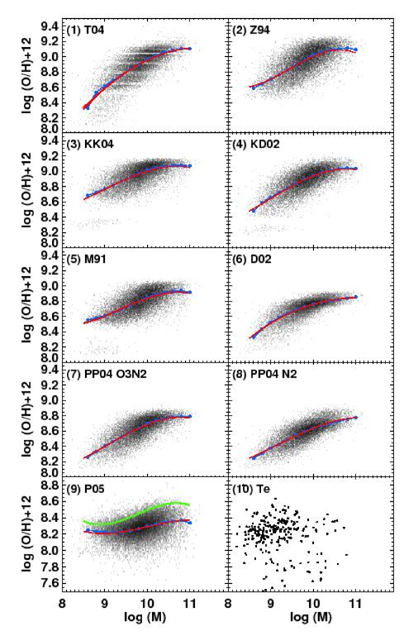
Figure 1.— The mass-metallicity relation using the 10 different metallicity calibrations listed in Table 1. The red line shows the robust best-fitting 3rd-order polynomial to the data. The blue circles give the median metallicity within stellar mass bins of $\Delta\log({\rm M}/$${\rm M}_{\odot}$$)=0.2$, centered at $\log({\rm M}/$${\rm M}_{\odot}$$)=8.6,8.8,...,11$. We use the updated calibration of P05 given by Pilyugin & Thuan (2005) in panel 9. The original P01 calibration is shown as a solid green line in panel 9.

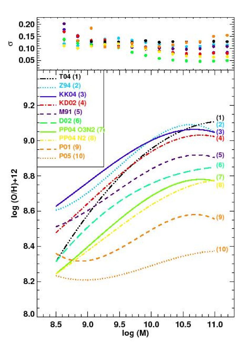
Figure 2.— The robust best-fit mass-metallicity relations calculated using the different metallicity calibrations listed in Table 1, except the T_e-method. The top panel shows the rms scatter in metallicity about the best-fit relation for each calibration in 0.1 dex bins of stellar mass. The y-axis offset, shape, and scatter of the MZ relation differs substantially, depending on which metallicity calibration is used.

We directly compare the best-fit MZ curves for the 9 strong-line calibrations in Figure 2, including both P01 and P05. The top panel shows the rms scatter in metallicity about the mean in mass bins of width $\Delta\log({\rm M}/$${\rm M}_{\odot}$$)=0.2$. The major difference between the MZ curves is their position along the y-axis. The curves with the largest y-intercept are all photoionization model based (KK04, Z94, KD02, T04, M91). Among these photoionization model metallicities, the agreement is $\sim 0.2$ dex. This agreement is within the margin of error typically cited for these calibrations ($\sim 0.1-0.15$ dex for each calibration). Some calibrations consistently agree to within 0.1 dex (e.g., KK04 and Z94; KD02 and M91). Comparisons between metallicities calculated using these consistent methods, such as KD02 and M91, are likely to be reliable to within 0.1 dex. However, comparisons between methods that show large disagreement (such as KK04 and P05) will be contaminated by the large systematic discrepancy between the calibrations.

The lowest curves in Figure 2 are the MZ relations derived using the empirical methods (i.e. P01, P05, and the two PP04 methods). These empirical methods are calibrated predominantly via fits of the relationship between strong-line ratios and H II region T_e metallicities. There is considerable variation among the y-intercept of these T_e-based MZ relations; the P05 method gives metallicities that are $\sim 0.4$ dex below the PP04 methods at the highest masses, despite the fact that both methods are predominantly based on H II regions with T_e-metallicities. At the lowest stellar masses, this difference disappears. The difference between the empirical methods may be attributed to the different H II-region samples used to derive the calibrations. At the highest metallicities, the PP04 methods utilize four H II-regions with detailed theoretical metallicities. These detailed theoretical metallicities may overcome the saturation at $12+\log({\rm O/H})$$\sim 8.6$ suffered by [O III] $\lambda 4363$ T_e metallicities. The P05 calibration includes some H II regions with metallicities estimated with the alternative auroral [N II] $\lambda 5755$ line from Kennicutt et al. (2003). The inclusion of these [N II] $\lambda 5755$ metallicities may overcome the [O III] $\lambda 4363$ saturation problem. However, Stasińska (2005) suggest that the use of the [N II] $\lambda 5755$ line in dusty nebulae will still cause T_e metallicities to be underestimated when the true metallicity is above solar. Our SDSS sample has a mean extinction of E(B-V)$\sim 0.3$, or $A_{V}\sim 1$. The extinction is a strong function of stellar mass; for the largest stellar masses (M$>10^{10.5}$${\rm M}_{\odot}$), the mean extinction is large E(B-V)$\sim 0.5$, or $A_{V}\sim 1.6$. Clearly, dust is important in SDSS galaxies, particularly at the highest stellar masses where the largest discrepancies exist between the theoretical methods and the P05 T_e-methods.

In addition to the large difference in y-intercept between the different metallicity calibrations, Figure 2 shows that the slope and turn-over of the MZ relation depend on which calibration is used. Therefore, it is essential to compare MZ relations that have been calculated using the same metallicity calibration. In the following section, we derive conversions that can be used to convert metallicities from one calibration into another.

6. Metallicity Calibration Conversions

Comparisons between MZ relations for galaxies in different redshift ranges are non-trivial. Different suites of emission-lines are available at different redshifts, necessitating the use of different metallicity calibrations. Because of the strong discrepancy in absolute metallicities between different calibrations, the application of different calibrations for galaxies at different redshifts may mimic or hide evolution in the MZ relation with redshift, depending on which calibrations are used. Because the metallicity discrepancies are systematic, we can fit the relationship between the different metallicity calibrations in order to remove the systematic discrepancies and obtain comparable metallicity measurements for different redshift intervals.

We calculate conversion relations between the strong-line metallicity calibrations by plotting each calibration against the remaining 8 calibrations and fitting the resulting metallicity-metallicity distribution with a robust polynomial fit. We refer to these metallicity-metallicity plots as Z-Z plots. Rows 1-3 of Figure 3 give six representative examples of SDSS Z-Z plots for the strong-line calibrations. The Z-Z plots between all nine strong-line calibrations for various S/N cuts are available at http://www.ifa.hawaii.edu/$\sim$kewley/Metallicity. The blue dashed 1:1 line shows where the Z-Z distribution would lie if the two calibrations agree. The robust best-fit polynomial is shown in red, and $\rho_{r}$ gives the robust equivalent to the standard deviation of the fit. Small values of $\rho_{r}$ indicate a reliable fit to the data.

The majority of the Z-Z relations are close to linear and are easily fit by a 1st, 2nd or 3rd order robust polynomial. However, the P05 calibration produces a very non-linear relation with a large scatter when plotted against all other metallicity calibrations. These non-linear relations are not easily fit even with a robust 3rd order polynomial and we cannot provide conversions that will reliably convert to/from the P05 method. For comparison, the bottom row of Figure 3 shows the same plots calculated with the original P01 calibration. Although the scatter is less severe in these plots, the relations between P01 and other diagnostics remain non-linear and are not easily fit with a robust 3rd order polynomial.

For all other diagnostics, the metallicities or metallicity relations can be converted into any other calibration scheme, using

$$y=a+bx+cx^{2}+dx^{3}$$ (1)

where $y$ is the ”base” or final metallicity in $12+\log({\rm O/H})$ units, $a-d$ are the 3rd order robust fit coefficients given in Table 3, and $x$ is the original metallicity to be converted (in $12+\log({\rm O/H})$ units). For Z-Z relations where a 2nd order polynomial produces a lower $\rho_{r}$ than a 3rd order polynomial fit, $d$ is zero.

The conversion coefficients given in Table 3 are based on the fit order that produces the lowest $\rho_{r}$ value in our sample. Some ${\rm R}_{23}$ calibrations require two fits; one 2nd or 3rd order fit for the upper ${\rm R}_{23}$ branch and one linear fit for the lower branch. In these cases, the coefficents of the upper and lower branch fits are listed in Table 3 as left and right columns, respectively.

In Table 3, we give the range in $x$ over which our calibrations are valid. Our polynomial fits are only tested within these ranges and may not be suitable for converting lower or higher metallicities into another scheme outside these limits. We provide worked examples for the use of our conversions in Appendix B.

Figure 4 shows the application of our strong-line conversions to the best-fit MZ relations in Figure 2, excluding P05. The calibration shown for each panel represents the “base” (final) calibration into which all other MZ curves have been converted. The remaining discrepancy between the converted MZ relation and the base MZ relation is an indicator of both the scatter in our Z-Z plots and how well the Z-Z relations are fit by a robust polynomial. In Table 4, we give the mean residual discrepancy between the converted MZ relations and the base MZ relation.

Our conversions reach agreement between the MZ relations to within $\sim 0.03$ dex on average. The most reliable base calibrations are those with the smallest residual discrepancies. The residual discrepancies differ because some Z-Z relations have less scatter and/or are more easily fit by a simple polynomial. The KK04, M91, PP04 O3N2, and KD02 methods have the smallest residual discrepancies and are therefore the most reliable base calibrations to convert other metallicities into.

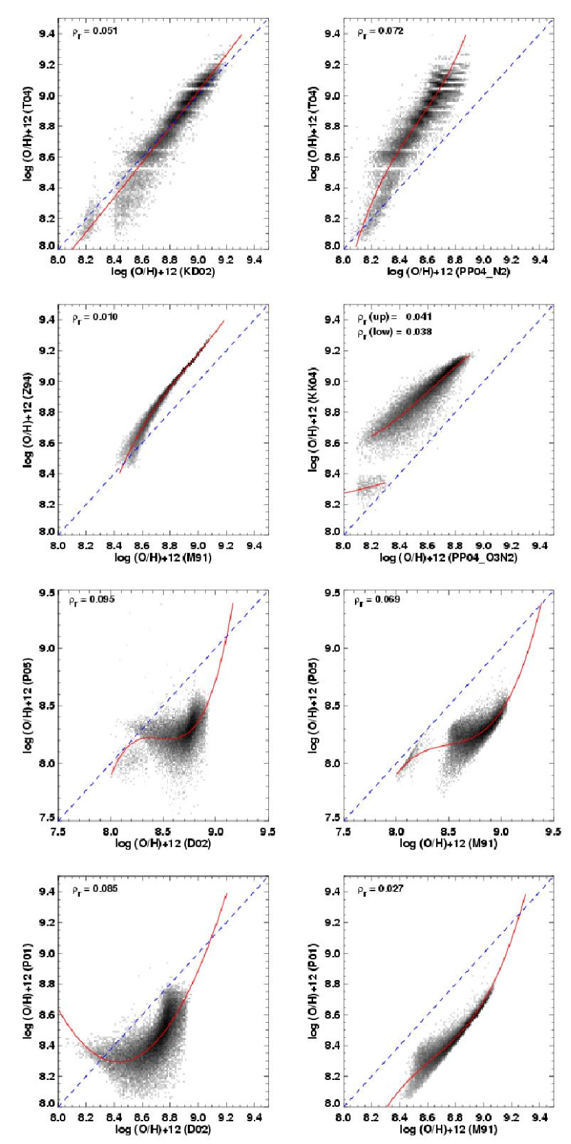
Figure 3.— Examples of the relationship between different metallicity calibrations. The robust 2nd order polynomial of best fit is shown as a red solid line. The 1:1 line (blue dashes) shows where the metallicities would lie if the calibrations agree. The robust equivalent to the standard deviation of the fit ($\rho_{r}$) are shown for each plot. This figure illustrates the typical variation in scatter and shape between different metallicity calibrations. Figures showing the relations between all 9 strong-line metallicity calibrations are available at http://www.ifa.hawaii.edu/$\sim$kewley/Metallicity.

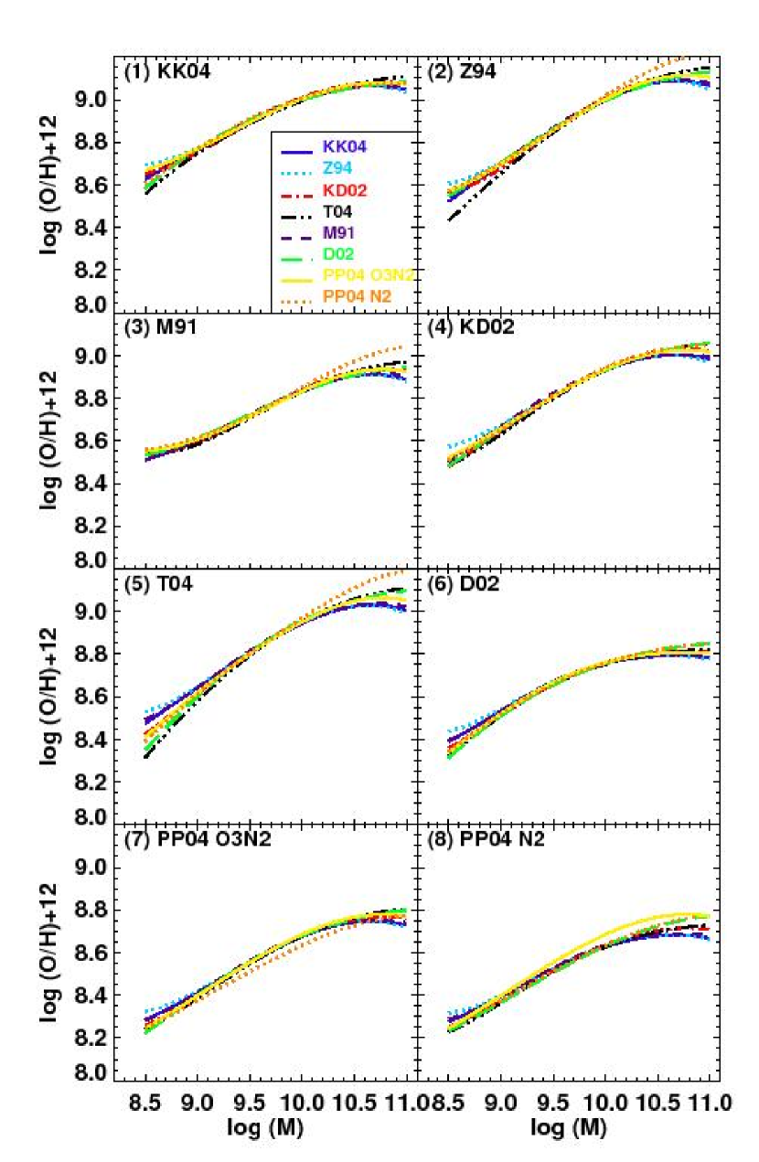
Figure 4.— The robust best-fit mass-metallicity relations calculated using the 8 different metallicity calibrations listed in Table 1, converted into the base metallicities shown using our conversions from Table 3.

7. The MZ Relation: AGN removal methods

The nebular emission line spectrum is sensitive to the hardness of the ionizing EUV radiation. Metallicities calculated from spectra that contain a significant contribution from an AGN may be spurious because the commonly-used metallicity calibrations are based on the assumption of a stellar ionizing radiation field. The standard optical diagnostic diagrams for classification were first proposed by Baldwin et al. (1981), based on the line ratios [N II]/H$\alpha$ vs [O III]/H$\beta$, [S II]/H$\alpha$ vs [O III]/H$\beta$, and [O I]/H$\alpha$ vs [O III]/H$\beta$. This classification scheme was revised by Osterbrock & Pogge (1985) and Veilleux & Osterbrock (1987, ; hereafter VO87) who used a combination of AGN and starburst samples with photoionization models to derive a classification line on the diagnostic diagrams to separate AGN from starburst galaxies. Subsequently, Kewley et al. (2001, ; hereafter Ke01) developed a purely theoretical “maximum starburst line” line for AGN classification using the standard diagrams. This theoretical scheme provides an improvement on the previous semi-empirical classification by producing a more consistent classification line from diagram to diagram that significantly reduces the number of ambiguously classified galaxies. The “maximum starburst line” defines the maximum theoretical position on the diagnostic diagrams that can be attained by pure star formation models. According to the Ke01 models, galaxies lying above the maximum starburst line are dominated by AGN activity and objects lying below the line are dominated by star formation.

Although objects lying below the maximum starburst line are likely to be dominated by star formation, they may contain a small contribution from an AGN. We calculate the maximum AGN contribution that would allow a galaxy to be classified as star-forming with the Ke01 line on all three standard diagnostic diagrams using theoretical galaxy spectra. Our AGN model is based on the $12+\log({\rm O/H})$$=8.9$ dusty radiation-pressure dominated models by (Groves et al., 2004). We use a typical AGN ionization parameter of $\log(U)=-2$ and a power-law index of $\alpha=-1.4$. We investigate the suite of starburst models from Kewley & Dopita (2002) and Dopita et al. (2000). The starburst model that allows the maximum contribution from an AGN while remaining classified as star-forming is zero-age instantaneous burst model with ionization parameter $q=1\times 10^{7}$ cm/s and metallicity $12+\log({\rm O/H})$$=8.9$ by (Kewley & Dopita, 2002; Dopita et al., 2000). The AGN contribution in this model is $\sim 15$%.

We use this model to calculate the effect of a 15% AGN contribution to the metallicity-sensitive emission-line ratios. The AGN model contributes substantially to the [O III]/H$\beta$ line ratio but has only a minor effect on the [N II]/[O II] ratio. Therefore, the effect of an AGN contribution of 15% is small ($\leq 0.04$ dex) on metallicities calculated using the [N II]/[O II] ratio (Kewley & Dopita, 2002), but larger ($0.1-0.2$ dex) on metallicities calculated with calibrations containing [O III] (e.g., McGaugh, 1991; Zaritsky et al., 1994; Kobulnicky & Kewley, 2004).

Recently, Kewley et al. (2006, ; hereafter Ke06) defined a new classification scheme based on all three diagnostic diagrams that separates pure HII region-like galaxies from HII-AGN composites, Seyferts, and galaxies dominated by low ionization emission line regions (LINERs). This new classification scheme includes an empirical shift applied by Kauffmann et al. (2003, ; hereafter Ka03) to the Ke01 line for the [N II]/H$\alpha$ vs [O III]/H$\beta$ diagnostic. This shift provides a more stringent removal of objects containing AGN, and we recommend its use for metallicities calculated using ${\rm R}_{23}$.

We investigate whether the AGN classification scheme affects the shape of the MZ relation in Figure 5. For each metallicity calibration, we show the MZ relation for the three classification schemes Ke01 (black dotted line), Ke06 (red solid line) and VO87 (blue dashed line). These three classification schemes define 89%, 84%, and 76% of our SDSS sample as star-forming, respectively. There is negligible difference ($<0.05$ dex) among the SDSS MZ relations for the three classification schemes. We note that the contribution from an AGN may be more important for samples that contain a larger fraction of HII-AGN composite galaxies, or galaxies at high redshift where limited sets of emission-lines limit the methods for AGN removal. For these cases, we recommend the use of either the KD02 [N II]/[O II] metallicity calibration (useful for log([N II]/[O II])$>-1.2$), the PP04 [N II]/H$\alpha$ calibration, or the D02 [N II]/H$\alpha$ calibration. None of these three calibrations depend on the AGN-sensitive [O III]/H$\beta$ line ratio.

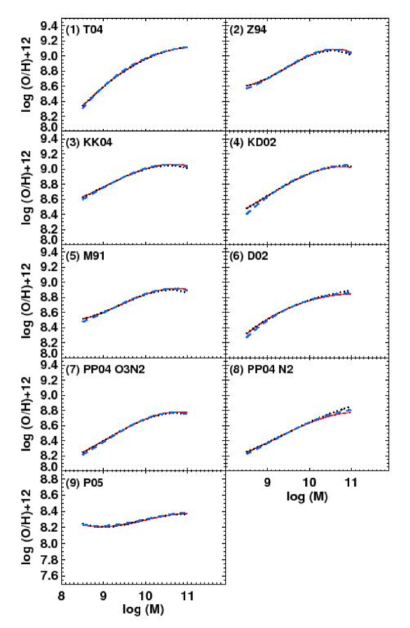
Figure 5.— Comparison between the mass-metallicity relations for three different methods of AGN removal: Kewley et al. (2006) (red solid line), Kewley et al. (2001) (black dotted line), and Veilleux & Osterbrock (1987) (VO87; blue dashed line). The method of AGN removal has little effect on the MZ relation, except at low stellar masses here the VO87 method gives a flatter slope.

8. The MZ Relation: Aperture Effects

Our SDSS sample was selected with g’-band covering fractions $>20$% because this value is the minimum covering fraction required for metallicities to approximate the global values (Kewley et al., 2005). A covering fraction of $20$% corresponds to a median redshift of $z\sim 0.04$ which is the lower redshift limit used by T04 for their SDSS MZ relation work. The median g’-band aperture covering fraction of our sample is only $\sim$34%, although the range of g’-band covering fractions is 20-80% (Figure 6).

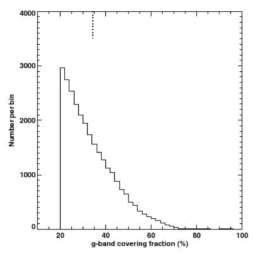
Figure 6.— The distribution of g’-band fiber covering fractions in our SDSS sample. Our sample was chosen to have covering fractions $>20$%. The dotted line at the top of the figure indicate the median (34.2) covering fraction of our sample.

Strong metallicity gradients exist in most massive late-type spirals; H II region metallicities decrease by an order of magnitude from the inner to the outer disk (see e.g., Shields, 1990, for a review). These gradients may cause substantial differences between the nuclear and global metallicities. Kewley et al. (2005) investigate the effects of a fixed size aperture on spectral properties for a large range of galaxy types and luminosity. They conclude that minimum covering fractions larger than $20$% may be needed at high luminosities to avoid aperture effects. Therefore the SDSS MZ relation may be affected by the fixed size aperture at the highest luminosities or stellar masses.

To investigate the effect of the small median SDSS covering fraction on the MZ relation, in Figure 7, we compare the SDSS MZ relation (red solid line) with the nuclear (black dot-dashed line) and global (blue dashed line) MZ relations of the Nearby Field Galaxy Survey (NFGS). We show the KD02 metallicity calibration (left panel) and the M91 calibration (right panel) for all datasets. Similar results are obtained with the other strong-line methods. The SDSS MZ relation lies in-between the NFGS nuclear and global relations at high stellar masses (${\rm M}>10^{10}$${\rm M}_{\odot}$). The NFGS global MZ relation flattens at a metallicity that is $\sim 0.1-0.15$ dex smaller than the metallicity at which the SDSS relation flattens. This difference is not caused by metallicity calibration errors because the difference in upper turn-off is observed with all strong-line metallicity calibrations. Furthermore, the difference of $\log({\rm M})=0.17$ dex between the Bell & de Jong (2001) stellar mass relation and the SDSS Bruzual & Charlot model stellar masses cannot account for the difference between the SDSS and global NFGS MZ relations.

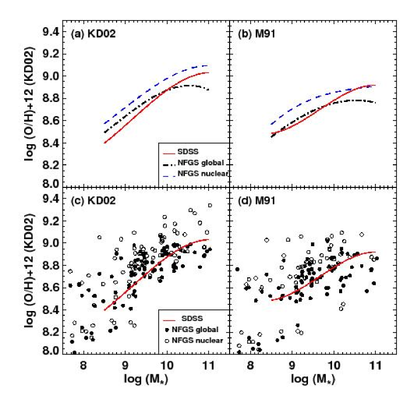
Figure 7.— (Top Panel) Comparison between the robust best-fit SDSS Mass-Metallicity relation (red solid line) and the best-fit relations to the Nearby Field Galaxy Survey (NFGS) nuclear (blue dashed line) and global (black dot-dashed line) relations. Metallicities were calculated using both KD02 (left panel) and M91 (right panel) calibrations, and stellar masses are given assuming a Salpeter IMF. (Bottom Panel) Comparison between the SDSS Mass-Metallicity relation (red solid line) and the NFGS global (filled circle) and NFGS nuclear (unfilled circle) data. At high stellar masses (${\rm M}_{*}>10^{10}$${\rm M}_{\odot}$), the SDSS metallicities are $\sim 0.1-0.15$ dex larger than NFGS global metallicities at the same stellar mass.

The difference between the SDSS and NFGS nuclear and MZ relations is probably driven by two factors: (1) fixed-size aperture differences and (2) different surface brightness profiles. The NFGS nuclear sample has a smaller mean covering fraction than the SDSS sample ($\sim 10$% c.f. $\sim 34$%), giving higher nuclear metallicities in the NFGS than for SDSS galaxies with the same stellar mass. In addition, the NFGS and SDSS samples have different surface brightness profiles (traced by their half-light radii). The NFGS sample has a slightly smaller mean half light radius than our SDSS sample ($\sim 3.0$ kpc c.f. $\sim 3.4$ kpc respectively). Ellison et al. (in prep.) show that for the SDSS, galaxies with small g’-band half light radii (i.e more concentrated emission) have higher metallicities at a given mass than galaxies with large half light radii (more diffuse emission).

The difference in half-light radii between the SDSS and NFGS samples can not explain the difference between SDSS galaxies and global NFGS MZ relations at high stellar masses ${\rm M}_{*}>10^{10}$${\rm M}_{\odot}$because (a) the larger mean half-light radii of the SDSS sample would bias the SDSS towards lower metallicities than the NFGS (Ellison et al. in prep), and (b) the NFGS global aperture covering fraction ($\sim 82$%) captures most of the NFGS B-band emission. The half-light radius is irrelevant when the spectrum captures 100% of the B-band light.

We conclude that a g’-band covering fraction of $\sim 20$% (or lower redshift limit of $z=0.04$) is insufficient for avoiding aperture bias in SDSS galaxies with stellar masses ${\rm M}_{*}>10^{10}$${\rm M}_{\odot}$. The mean covering fraction for ${\rm M}_{*}>10^{10}$${\rm M}_{\odot}$ galaxies is $30.6\pm 0.1$%. A larger mean covering fraction is required to obtain a reliable MZ relation at ${\rm M}_{*}>10^{10}$${\rm M}_{\odot}$.

9. Discussion

We have investigated the effect of metallicity calibrations, AGN removal schemes, and a fixed-size aperture on the MZ relation. The choice of metallicity calibration has the strongest effect on the MZ relation. The choice of metallicity calibration changes the y-intercept of the MZ relation significantly; the discrepancy between the metallicity calibrations is as large as $0.7$ dex at the highest stellar masses. This discrepancy corresponds to a difference of 0.5 to $2.6\times$ solar at the peak metallicity of our SDSS sample.

The existence of a $\sim 0.4-0.5$ dex discrepancy between the T_e and theoretical metallicities is well known (Stasińska, 2002; Kennicutt et al., 2003; Garnett et al., 2004b). Our results show that the discrepancy is larger than previously thought. This discrepancy is often interpreted as an unknown problem with the photoionization codes used to calibrate the strong line ratios with metallicity (Kennicutt et al., 2003; Garnett et al., 2004b; Tremonti et al., 2004). However, recent investigations indicate that the T_e methods may underestimate the metallicity when temperature fluctuations or gradients exist within the emission-line nebulae (Stasińska, 2005; Bresolin, 2006a). These fluctuations, and hence the effect on T_e  are expected be the strongest at the highest metallicities. We conclude that for the metallicities spanned by the SDSS sample, it is not possible to know which (if any) metallicity calibration is correct. Until the metallicity discrepancies are resolved, only relative metallicity comparisons should be made.

Relative metallicity comparisons rely on the ability of strong-line calibrations to consistently reproduce the metallicity difference between any two galaxies. For example, if two galaxies have metallicities of $12+\log({\rm O/H})$$=8.4$ and $12+\log({\rm O/H})$$=8.9$ using one metallicity calibration, the difference in relative metallicities (0.5 dex) should be the same using any other metallicity calibration, even if the absolute metallicities differ from one calibration to another. We test how well the strong-line metallicity calibrations maintain relative metallicities by selecting $30,000$ random sets of two galaxies from our SDSS sample. We measure the relative metallicity difference between the two galaxies from each set for each metallicity calibration. We give the mean difference in relative metallicity and rms residuals in Table 5. The mean difference in relative metallicity is $<0.07$ dex for all strong-line metallicity calibrations. The rms scatter is $\lesssim 0.15$ dex for all calibrations. The P05 method gives more discrepant relative metallicities to the other strong-line methods, with relative metallicity differences between $0.08-0.14$ dex rms (c.f. 0.02 - 0.11 dex rms). The best agreement between relative metallicities occurs between the three theoretical ${\rm R}_{23}$ calibrations (M91, Z94, KK04), with relative metallicities agreeing to within $0.02-0.05$ dex rms. The small difference and rms residuals in relative metallicities for all 9 strong-line calibrations indicates that comparisons between galaxy or H II-region metallicities can be reliably made to within $\sim 0.15$ dex, as long as the same base metallicity calibration is used for galaxies or H II regions. Our metallicity conversions aid relative metallicity comparisons between different samples of galaxies at different redshifts by empirically removing the discrepancy between each metallicity calibration. In practice, if relative metallicity differences between galaxies or between samples is $\lesssim 0.15$ dex, we recommend the use of two or more metallicity calibrations to verify that any difference observed is real, and not introduced by the metallicity calibration applied.

The SDSS sample is insufficient for determining the cause(s) of the metallicity discrepancy problem. Several ongoing investigations into the metallicity discrepancies may help solve this problem in the near future. These investigations include tailored photoionization models, high S/N spectroscopy of luminous stars in the Milky Way and nearby galaxies, metal recombination lines, IR fine structure lines, and temperature fluctuation studies.

Garnett et al. (2004a) applied tailored photoionization models to optical and infrared spectra of the H II region CCM 10 in M51. They found that the CCM 10 metallicity derived from the electron temperature using the infrared [O III] 88$\mu$m line agrees with the theoretical metallicity computed with the latest version of the CLOUDY v90.4 photoionization code (Ferland et al., 1998). This theoretical metallicity is a factor of 2 smaller than the metallicity calculated with the previous version of CLOUDY (v. 74) that uses older atomic data. Clearly the optical emission-line strengths in the photoionization models are very sensitive to the atomic data used. However, this sensitivity cannot explain the discrepancy observed in Figure 2 because T04 used the same version of Cloudy as Garnett et al. In spite of the use of modern photoionization models with more accurate atomic data, the T04 MZ relation lies significantly higher than the methods utilizing T_e metallicities (P05,D02,PP04). Mathis & Wood (2005) used Monte Carlo photoionization models to show that different density distributions are not a significant source of error on the theoretical abundances. Recently, Ercolano et al. (2007) used new 3D photoionization codes to investigate the effect of multiply non-centrally located stars on the temperature and ionization structure of H II regions. Ercolano et al. suggest that the geometrical distribution of ionizing sources may affect the metallicities derived using theoretical methods. Further theoretical investigations into the model assumptions, as well as tailored photoionization model fits to multi-wavelength data of spatially resolved star-forming regions may yield clues into whether the theoretical models contribute to the metallicity discrepancy.

High S/N spectroscopy with 8-10m telescopes can now provide metallicities for luminous stars and planetary nebulae in nearby galaxies that can be compared with H II region metallicities (see Przybilla et al., 2007, for a review). Urbaneja et al. (2005) analysed the chemical composition of B-type supergiant stars in M33. They find that the supergiant metallicities agree with H II region abundances derived using the T_e- method. Similar results were obtained for local dwarf galaxies (Bresolin et al., 2006), however other investigations require a correction for electron temperature fluctuations before agreement can be reached (Simón-Díaz et al., 2006).

Metal recombination lines provide a promising independent baseline for metallicity measurements because metal recombination lines depend only weakly on T_e(Bresolin, 2006a, see e.g.,). Metal recombination lines are weak, but they have been observed in H II regions in the Milky Way (Esteban et al., 2004, 2005; García-Rojas et al., 2005, 2006), and recently in nearby galaxies (Esteban et al., 2002; Peimbert et al., 2005). Recombination methods typically agree with theoretical methods (e.g., Bresolin, 2006a), and predict larger metallicities (by 0.2-0.3 dex) than the T_e method. When the T_e metallicities are corrected for electron temperature fluctuations, agreement is reached between recombination and T_e methods (Peimbert et al., 2005; García-Rojas et al., 2005, 2006; Peimbert et al., 2006; López-Sánchez et al., 2007).

Measurements of electron temperature fluctuations in nearby H II regions can resolve the disagreement between strong-line theoretical methods, and electron temperature methods (García-Rojas et al., 2006; Bresolin, 2007) in most cases (see however Hägele et al., 2006). More electron temperature measurements are needed to verify these results, particularly for high metallicity H II regions where electron temperature fluctuation measurements are lacking.

Despite these promising investigations, the metallicity discrepancy problem remains unsolved at the present time. Until the metallicity discrepancy problem is resolved, absolute metallicity values should be used with caution. In Table 5, we show that the metallicity calibrations maintain relative metallicities better than $\sim 0.15$ dex rms, with the majority of theoretical methods maintaining relative metallicities within $0.04-0.1$ dex rms. Therefore, studies of relative metallicity differences, such as comparisons between different galaxy samples, or between individual galaxies or H II regions, can be reliably made. If the size of the differences observed between different samples or different objects is $\sim 0.15$ dex or less, we recommend the use of at least two independent calibrations to verify that the difference is calibration-independent. The KD02 and PP04 methods give (a) low residual discrepancies in relative metallicities, and (b) low residual discrepancy after other metallicities have been converted into these two methods. For the metallicity range of the SDSS sample, the KD02 and PP04 N2 calibrations are also independent of small contributions from an AGN. Because the KD02 and PP04 O3N2 methods maintain robust relative metallicities and are good base calibrations, we recommend the use of these two methods when deriving relative metallicities.

10. Conclusions

We present a detailed investigation into the mass-metallicity relation for 27,730 star-forming galaxies from the Sloan Digital Sky Survey. We apply 10 different metallicity calibrations to our SDSS sample, including theoretical photoionization calibrations and empirical T_e method calibrations. We investigate the effect of these metallicity calibrations on the shape and y-intercept of the mass-metallicity relation. Using 30,000 galaxy sets sampled randomly from our SDSS sample, we investigate how well the 9 strong-line calibrations maintain relative metallicities. We find that:

• The choice of metallicity calibrations has the strongest effect on the MZ relation. The choice of metallicity calibration can change the y-intercept of the MZ relation by up to 0.7 dex. Until this metallicity discrepancy problem is resolved, absolute metallicities should be used with extreme caution.

• There is considerable variation in shape and y-intercept of the MZ relations derived using the empirical methods. We attribute this variation to the different H II region samples used to derive the empirical calibrations.

• The relative difference in metallicities is maintained to an accuracy of $12+\log({\rm O/H})$$\sim 0.02-0.1$ dex for 9/10 calibrations, and to within $12+\log({\rm O/H})$$\sim 0.15$ dex for all 9 strong-line calibrations. For relative metallicity studies where the difference between targets or between samples is $\lesssim 0.15$ dex, we recommend the use of at least two different calibrations to check that any result is not caused by the metallicity calibrations.

We use robust fits to the observed relationship between each metallicity calibration to derive new conversion relations for converting metallicities calculated using one calibration into metallicities of another, ”base” calibration. We show that these conversion relations successfully remove the strong discrepancies observed in the MZ relation between the different calibrations. Agreement is reached to within 0.03 dex on average.

We investigate the effect of AGN classification scheme and fixed-size aperture on the MZ relation.

• AGN classification methods have a negligible effect on metallicities derived using [N II]/[O II] or [N II]/H$\alpha$. AGN classification can affect metallicities derived with ${\rm R}_{23}$ by $\lesssim 0.15$ dex. For the SDSS sample, AGN classification methods make negligible difference in the shape or y-intercept of the MZ relation. For samples containing a larger fraction of starburst-AGN composite galaxies, or samples where AGN removal is not possible, we recommend the use of [N II]/[O II] or [N II]/H$\alpha$ metallicity diagnostics.

• The median g’-band aperture covering fraction of our SDSS sample is 34.2%. This covering fraction is insufficient for metallicities to represent global values at high masses (M$>10^{10}$${\rm M}_{\odot}$). The Nearby Field Galaxy global MZ is $0.1-0.15$ dex lower than the SDSS MZ relation at M$>10^{10}$${\rm M}_{\odot}$. Therefore, the metallicity at which the SDSS MZ relation turns over is dependent on both the choice of metallicity calibration, and on the aperture size.

We recommend that metallicities be converted into either the Pettini & Pagel (2004) method or the Kewley & Dopita (2002) method to minimize any residual discrepancies, and to maintain accurate relative metallicities compared to other calibrations. These two diagnostics have the added benefit that at high metallicities, the Kewley & Dopita [N II]/[O II] and Pettini & Pagel [N II]/H$\alpha$ calibrations are relatively independent of the method used to remove AGN.

Future work into tailored photoionization models, high S/N spectroscopy of luminous stars in the Milky Way and nearby galaxies, metal recombination lines, IR fine structure lines, and temperature fluctuation studies may help resolve the metallicity discrepancy problem in the near future. Until then, only relative metallicity comparisons are reliable.

Appendix A Metallicity Calibrations: Equations and Method

A.1. Breaking the ${\rm R}_{23}$ Degeneracy

Many empirical and theoretical metallicity calibrations rely on the ([O II] $\lambda$3727 +[O III] $\lambda\lambda$4959,5007)/H$\beta$ line ratio, known as “${\rm R}_{23}$”. The major drawback to using ${\rm R}_{23}$ is that it is double-valued with metallicity; ${\rm R}_{23}$ gives both a low metallicity estimate (“lower branch”) and a high estimate (“upper branch”) for most values of ${\rm R}_{23}$ (see e.g., Kobulnicky & Kewley, 2004, for a discussion). Additional line ratios, such as [N II]/H$\alpha$, or [N II]/[O II], are required to break this degeneracy.

The SDSS catalog contains very few metal-poor galaxies (Izotov et al., 2004; Kniazev et al., 2003, 2004; Papaderos et al., 2006; Izotov et al., 2006a). Metal poor galaxies are often lacking in magnitude-limited emission-line surveys because they are intrinsically rare, compact and faint (e.g., Terlevich et al., 1991; Masegosa et al., 1994; van Zee, 2000). For the purpose of investigating the upper and lower ${\rm R}_{23}$ branches, we supplement the SDSS sample with (a) the low metallicity galaxy sample described in Kewley et al. (2007) and Brown et al. (2006), and (b) the Kong & Cheng (2002) blue compact galaxy sample.

Note that we do not calculate an initial metallicity from an [N II]/H$\alpha$ or [N II]/[O II] metallicity calibration because in some cases, a systematic discrepancy between a metallicity calibration based on [N II]/H$\alpha$ or [N II]/[O II]  and the calibration based on ${\rm R}_{23}$ will cause galaxies to be improperly placed on the upper or lower branch of ${\rm R}_{23}$. For example, an [N II]/H$\alpha$ metallicity calibration that systematically produces higher estimates than the subsequent ${\rm R}_{23}$ calibration may cause metallicities to be erroneously estimated from the upper ${\rm R}_{23}$ branch.

We use the [N II]/[O II] ratio to break the ${\rm R}_{23}$ degeneracy for our SDSS sample. The [N II]/[O II] ratio is not sensitive to ionization parameter to within ($\pm 0.05$ dex), and it is a strong function of metallicity above log([N II]/[O II])$\gtrsim-1.2$ (Kewley & Dopita, 2002). Figure 8a shows that the division between the ${\rm R}_{23}$ upper and lower branches occurs at log([N II]/[O II])$\sim-1.2$ for the SDSS and supplementary samples. For comparison, Figure 8b shows the theoretical relationship between [N II]/[O II] and ${\rm R}_{23}$ using the population synthesis and photoionization models of Kewley & Dopita (2002). The observed ${\rm R}_{23}$ peak at log([N II]/[O II])$\sim-1.2$ corresponds to a metallicity of $12+\log({\rm O/H})$$\sim 8.4$ according to the theoretical models.

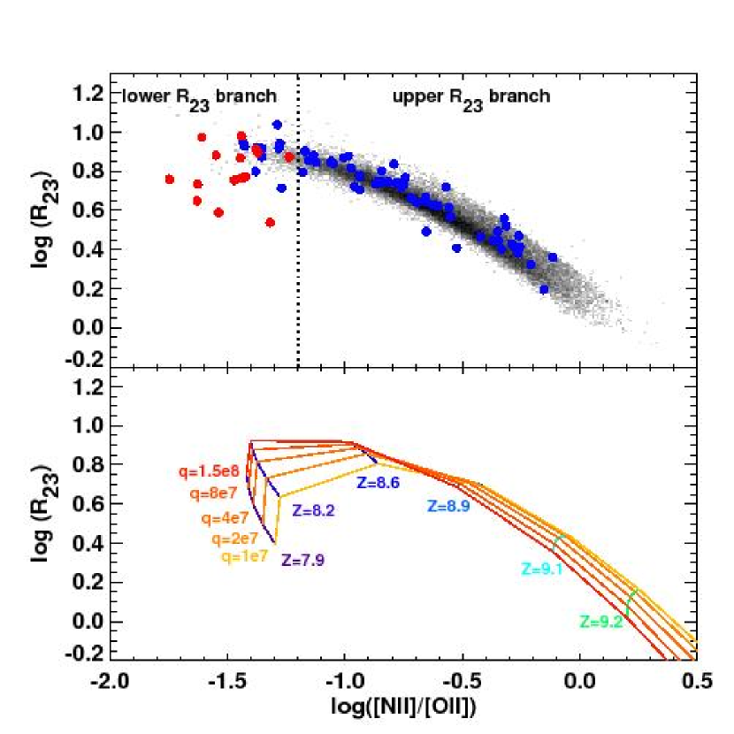
Figure 8.— (a) The observed relationship between the metallicity-sensitive [N II] $\lambda$6584/[O II] $\lambda$3727 line ratio and the commonly-used ([O II] $\lambda$3727 +[O III] $\lambda\lambda$4959,5007)/H$\beta$ ratio. The SDSS galaxies (black), the Kong & Cheng (2002) blue compact galaxy sample (blue) and the Brown et al. (2006) low metallicity galaxy samples (red) are shown. The [NII]/[OII] ratio is a strong monotonic function of metallicity to log([NII]/[OII])$\gtrsim-1.2$, while ${\rm R}_{23}$ has a maximum at log(${\rm R}_{23}$ )$\sim 0.9$. For our samples, the ${\rm R}_{23}$ maximum is likely to occur at log([NII]/[OII])$\sim-1.2$. This value can be used to break the ${\rm R}_{23}$ degeneracy for galaxies where [NII]/[OII] can be corrected for extinction using the Balmer Decrement. (b) The theoretical relationship between the [NII]/[OII] and ${\rm R}_{23}$ line ratios using the stellar population synthesis and photoionization model grids of Kewley & Dopita (2002). Models are shown for constant metallicities of $12+\log({\rm O/H})$$=7.9,8.2,8.6,8.9,9.1,9.2$ and ionization parameters of $q=1\times 10^{7},\,2\times 10^{7},\,4\times 10^{7},\,8\times 10^{7},1.5\times 10^{8}$ $cm\,s^{-1}$. We choose a break between the ${\rm R}_{23}$ upper and lower branches at log([NII]/[OII])$\sim-1.2$, which corresponds to a metallicity of $12+\log({\rm O/H})$$\sim 8.4$ according to the theoretical models.

For galaxies at high redshift, the [N II]/[O II] ratio cannot be used to break the ${\rm R}_{23}$ degeneracy because either (a) [N II]/[O II] cannot be corrected for extinction due to a lack of reliable Balmer line ratios, and/or (b) [N II] and [O II] are not observed simultaneously in a given spectrum. In this case the [N II]/H$\alpha$ ratio is used (Figure 9). Figure 9a shows that the division between the ${\rm R}_{23}$ upper and lower branches occurs between $-1.3<$log([N II]/H$\alpha$)$\lesssim-1.1$ for the SDSS and supplementary samples. The division between the upper and lower ${\rm R}_{23}$ branches using [N II]/H$\alpha$ (Figure 9a) is less clear than for [N II]/[O II] (Figure 8a) because the [N II]/H$\alpha$ ratio is less sensitive to metallicity, and more sensitive to ionization parameter, than [N II]/[O II].

We check whether our empirical [N II]/H$\alpha$ division between the upper and lower ${\rm R}_{23}$ branches $-1.3<$log([N II]/H$\alpha$)$\lesssim-1.1$ is compatable with our [N II]/[O II] division (log([N II]/[O II])$\lesssim-1.2$) by comparing the number of galaxies placed on the upper and lower branches using each ratio. For log([N II]/H$\alpha$)$\lesssim-1.3$, the majority of galaxies (150/175; 86%) lie on the lower ${\rm R}_{23}$ branch according to their [N II]/[O II] line ratios. For log([N II]/H$\alpha$)$\gtrsim-1.1$, the upper ${\rm R}_{23}$ branch can be clearly seen. For $-1.3<$log([N II]/H$\alpha$)$<-1.1$, [N II]/H$\alpha$ cannot discriminate between the upper and lower ${\rm R}_{23}$ branches. Figure 9b shows that galaxies with $-1.3<$log([N II]/H$\alpha$)$<-1.1$ are likely to have metallicities that are close to the ${\rm R}_{23}$ maximum. For the SDSS galaxies with $-1.3<$log([N II]/H$\alpha$)$<-1.1$ in Figure 9a, the [N II]/[O II] ratios indicate that 634/1127 (56%) of SDSS galaxies lie on the upper branch and 493/1127 (44%) SDSS galaxies lie on the lower branch.

For the ${\rm R}_{23}$ methods in this paper, we use the [N II]/[O II] line ratio to break the ${\rm R}_{23}$ degeneracy.

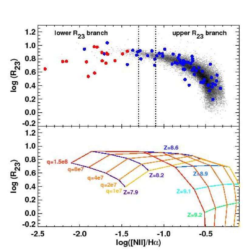
Figure 9.— (a) The observed relationship between the metallicity-sensitive [N II] $\lambda$6584/H$\alpha$ line ratio and the commonly-used ([O II] $\lambda$3727 +[O III] $\lambda\lambda$4959,5007)/H$\beta$ ratio. The SDSS galaxies (black), the Kong & Cheng (2002) blue compact galaxy sample (blue) and the Brown et al. (2006) low metallicity galaxy samples (red) are shown. For log([NII]/H$\alpha$) $\gtrsim-1.1$, galaxies are likely to lie on the upper ${\rm R}_{23}$ branch. For $-1.3<$log([NII]/H$\alpha$ )$<-1.1$, [NII]/H$\alpha$ cannot discriminate between the upper and lower ${\rm R}_{23}$ branches. For log([N II]/H$\alpha$)$\lesssim-1.3$, galaxies lie on the lower ${\rm R}_{23}$ branch. (b) The theoretical relationship between the [N II]/[O II] and ${\rm R}_{23}$ line ratios using the stellar population synthesis and photoionization model grids of Kewley & Dopita (2002). Models are shown for constant metallicities of $12+\log({\rm O/H})$$=7.9,8.2,8.6,8.9,9.1,9.2$ and ionization parameters of $q=1\times 10^{7},\,2\times 10^{7},\,4\times 10^{7},\,8\times 10^{7},1.5\times 10^{8}$ $cm\,s^{-1}$.

A.2. Theoretical Photoionization Methods

A.2.1 McGaugh (1991) - M91

The McGaugh (1991) calibration of ${\rm R}_{23}$ is based on detailed H II region models using the photoionization code CLOUDY (Ferland et al., 1998). The M91 calibration includes a correction for ionization parameter variations. We use the [N II]/[O II] line ratio to break the ${\rm R}_{23}$ degeneracy, as described in Section A.1, and we apply the analytic expressions for the M91 lower and upper branches given in Kobulnicky et al. (1999):

$$12+\log({\rm O/H})_{lower} = 12-4.944+0.767x+0.602x^{2}$$ (A1)

$$-y(0.29+0.332x-0.331x^{2})$$

$$12+\log({\rm O/H})_{upper} = 12-2.939-0.2x-0.237x^{2}$$ (A2)

$$-0.305x^{3}-0.0283x^{4}-y(0.0047$$

$$-0.0221x-0.102x^{2}-0.0817x^{3}$$

$$-0.00717x^{4})$$

where $x=\log({\rm R_{23}})=\log\left(\frac{{\rm[OII]}\lambda 3727+{\rm[OIII]}\lambda 4959+{\rm[OIII]}\lambda 5007}{{\rm H}\beta}\right)$, and $y=\log({\rm O_{32}})=\log\left(\frac{{\rm[OIII]\lambda 4959}+{\rm[OIII]\lambda 5007}}{{\rm[OII]}\lambda 3727}\right)$. The estimated accuracy of the M91 calibration is $\sim 0.15$ dex.

A.2.2 Kewley & Dopita (2002) - KD02

The Kewley & Dopita (2002) calibrations are based on a self-consistent combination of detailed stellar population synthesis and photoionization models. The estimated accuracy of the KD02 calibrations is $\sim 0.1$ dex. This estimate is derived by varying the major assumptions in the stellar evolution and photoionization models (including the star formation prescription, electron density, and the initial mass function). KD02 outlined a “recommended” approach to deriving metallicities that uses the [N II]/[O II] line ratio for high metallicities and a combination of ${\rm R}_{23}$ calibrations for lower metallicities. We use a revised version of the KD02 calibration. For log([N II]/[O II])$>-1.2$ , we use the original KD02 [N II]/[O II] metallicity calibration given by

$$\log([NII]/[OII])=1106.8660-532.15451Z+96.373260Z^{2}-7.8106123Z^{3}+0.23928247Z^{4}$$ (A3)

where $Z=\log(O/H)+12$. We use the IDL task fz_roots to solve the 4th order polynomial for $Z$. The coefficients in Equation A3 are based on the theoretical $q=2\times 10^{7}$ cm/s relationship between [N II]/[O II]and $Z$. However, the detailed relationship between [N II]/[O II]and $Z$ is independent of ionization parameter to within $\sim 0.1$ dex for log([N II]/[O II])$>-1.2$ and the ionization parameters covered by the SDSS ($q=1\times 10^{7}-8\times 10^{7}$ cm/s).

For log([N II]/[O II])$<-1.2$ (or KD02 $12+\log({\rm O/H})$$<8.4$), KD02 recommend using an average of ${\rm R}_{23}$ methods. In this regime, we use the average of the KK04 lower banch ${\rm R}_{23}$ calibration (equation A6) and the lower branch M91 ${\rm R}_{23}$ calibration (equation A1). Both of these calibrations correct for ionization parameter variations.

A.2.3 Kobulnicky & Kewley (2004) - KK04

Kobulnicky & Kewley (2004) use the stellar evolution and photoionization grids from Kewley & Dopita (2002) to produce an improved fit to the ${\rm R}_{23}$ calibration. The estimated accuracy of the KK04 method is $\sim 0.15$ dex.

The ${\rm R}_{23}$ calibration is sensitive to the ionization state of the gas, particularly for low metallicities where the ${\rm R}_{23}$ line ratio is not a strong function of metallicity. The ionization state of the gas is characterized by the ionization parameter, defined as the number of hydrogen ionizing photons passing through a unit area per second, divided by the hydrogen density of the gas. The ionization parameter $q$ has units of cm/s and can be thought of as the maximum velocity ionization front that a radiation field is able to drive through the nebula. The ionization parameter is typically derived using the [O III]/[O II] line ratio. This ratio is sensitive to metallicity and therefore KK04 recommend an iterative approach to derive a consistent ionization parameter and metallicity solution. We first use the [N II]/[O II] ratio to determine whether each SDSS galaxy lies on the upper or lower ${\rm R}_{23}$ branch. We then calculate an initial ionization parameter by assuming a nominal lower branch ($12+\log({\rm O/H})$$=8.2$) or upper branch ($12+\log({\rm O/H})$$=8.7$) metallicity using equation (13) from KK04, i.e.

$$\log(q) = \{32.81-1.153y^{2}$$ (A4)

$$+[12+\log({\rm O/H})](-3.396-0.025y+0.1444y^{2})\}$$

$$\times\{4.603-0.3119y-0.163y^{2}$$

$$+[12+\log({\rm O/H})](-0.48+0.0271y+0.02037y^{2})\}^{-1}$$

where $y=\log O_{32}=\log\left({[{\rm OIII}]\,\lambda 5007}/{[{\rm OII}]\,\lambda 3727}\right)$. The initial resulting ionization parameter is used to derive an initial metallicity estimate from KK04 equation (16) for log([N II]/[O II])$<-1.2$ ($12+\log({\rm O/H})$$\lesssim 8.4$), or KK04 equation (17) for log([N II]/[O II])$>-1.2$ ($12+\log({\rm O/H})$$\gtrsim 8.4$):

$$12+\log({\rm O/H})_{lower} = 9.40+4.65x-3.17x^{2}$$ (A5)

$$-\log(q)(0.272+0.547x-0.513x^{2})$$

$$12+\log({\rm O/H})_{upper} = 9.72-0.777x-0.951x^{2}-0.072x^{3}-0.811x^{4}x$$ (A6)

$$-\log(q)(0.0737-0.0713x-0.141x^{2}+0.0373x^{3}-0.058x^{4})$$

where $x=\log{\rm R}_{23}=\log\left(\frac{[{\rm OII}]\,\lambda 3727+[{\rm OIII}]\,\lambda\lambda 4959,5007}{H\beta}\right)$. Equations A4 and A6 (or A5) are iterated until $12+\log({\rm O/H})$ converges. Three iterations are typically required to reach convergence.

A.2.4 Zaritsky et al. (1994) - Z94

The Zaritsky et al. (1994) calibration is based on the ${\rm R}_{23}$ line ratio. This calibration is derived from the average of three previous calibrations by Edmunds & Pagel (1984); Dopita & Evans (1986); McCall et al. (1985). The uncertainty in the Z94 calibration is estimated by the difference in metallicity estimates between the three calibrations. Z94 provide a polynomial fit to their calibration that is only valid for the upper ${\rm R}_{23}$ branch (i.e. $12+\log({\rm O/H})$$>8.4$, or log([N II]/[O II])$>-1.2$).

$$12+\log({\rm O/H})=9.265-0.33x-0.202x^{2}-0.207x^{3}-0.333x^{4}$$ (A7)

where $x=\log{\rm R}_{23}=\log\left(\frac{[{\rm OII}]\,\lambda 3727+[{\rm OIII}]\,\lambda\lambda 4959,5007}{H\beta}\right)$. A solution for the ionization parameter is not explicitly included in the Z94 calibration.

A.2.5 Tremonti et al. (2004) - T04

T04 estimated the metallicity for each galaxy statistically based on theoretical model fits to the strong emission-lines [O II], H$\beta$, [O III], H$\alpha$, [N II], [S II]. The model fits were calculated using a combination of stellar population synthesis models from Bruzual & Charlot (2003) and CLOUDY photoionization models Ferland et al. (1998). The T04 scheme is more sophisticated than the other theoretical methods because it takes advantage of all of the strong emission lines in the optical spectrum, allowing more constraints to be made on the model parameters. Calibrations of various line ratios to the theoretical T04 method are given by Nagao et al. (2006) and Liang et al. (2006). We use the original T04 metallicities, available from http://www.mpa-garching.mpg.de/SDSS/ for this study.

A.3. T_e method

We derive the gas-phase oxygen abundance following the procedure outlined in Izotov et al. (2006b). This procedure utilizes the electron-temperature (T_e) calibrations of Aller (1984) and the atomic data compiled by Stasińska (2005). Abundances are determined within the framework of the classical two-zone HII-region model (Stasińska, 1980). The ratio of the auroral [O III] $\lambda 4363$ and [O III] $\lambda\lambda 4959,5007$ emission-lines gives an electron temperature in the O⁺⁺ zone. We derive electron densities measured using the [S II] $\lambda 6717$/[S II] $\lambda 6731$ line ratio. These electron temperatures are insensitive to small variations in electron density; we obtain the same ${\rm T_{e}}$ with an electron density of 367 cm^-3. The electron temperature of the O⁺ zone is calculated assuming ${\rm T_{e}}({\rm O}^{+})=0.7\,{\rm T_{e}}({\rm O}^{++})+0.3$ (Stasińska, 1980). We calculate the metallicity in the O⁺ and O⁺⁺ zones assuming

$${\rm O/H}={\rm O}^{+}/{\rm H}^{+}+{\rm O}^{++}/{\rm H}^{+}$$ (A8)

The uncertainty in the absolute O/H metallicity determination by this T_e method is $\sim 0.1$ dex. This intrinsic uncertainty is the dominant error in our T_e metallicity determination, and includes errors in the use of simplified H II region models and possible problems with electron temperature fluctuations (Pagel & Tautvaisiene, 1997). Fortunately, these errors affect all T_e-based methods in a similar way and the error in relative metallicities derived using the same method is likely to be $<<0.1$ dex.

This “classical” T_e approach does not take unseen stages of ionization or electron temperature fluctuations into account. Bresolin (2006a) notes that if electron temperature fluctuations are substantial and are not taken into account, T_e-based calibrations can only provide a lower limit to the true metallicity, particularly in the high metallicity regime where T_e fluctuations appear stronger. We find that the T_e method does not produce any SDSS metallicities of solar ($12+\log({\rm O/H})$$\sim 8.69$; Allende Prieto et al., 2001; Asplund et al., 2004) or above, even for galaxies where the fiber only captures $20-30$% of the central g’-band galaxy light. Covering fractions of $20-30$% correspond to diameters of $\sim 5$ kpc for the mean size of nearby star-forming galaxies (Kewley et al., 2005). Spiral galaxies typically have metallicities within similar apertures that are $\sim 1-2\times$solar, measured using various independent methods (see Henry & Worthey, 1999, for a review). For example, our Galaxy has consistent central metallicities within the central $\sim 5$ kpc of $1-2\times$solar from studies of planetary nebulae (Martins & Viegas, 2000), IR fine structure lines in H II regions (Simpson et al., 1995; Afflerbach et al., 1997), and radio recombination lines (Quireza et al., 2006).

We conclude that T_e metallicities should be used with caution when other line ratios (such as [N II]/H$\alpha$ and [N II]/[O II]) indicate upper branch (Figures 8 and 9) or supersolar metallicities.

A.4. Empirical T_e fit methods

H II regions with electron temperature-based metallicities have been used in many studies to derive empirical fits to strong-line ratios that can be applied to H II regions and galaxies where the [O III] $\lambda$4363 line is not observed.

A.4.1 Pettini & Pagel (2004) - PP04 O3N2 & N2

Pettini & Pagel (2004) derived two new methods for measuring metallicities in galaxies at high redshift. At high redshift, obtaining a reddening estimate is difficult and in some cases, impossible, and flux calibration in the infrared is non-trivial. Ratios of lines that are very close in wavelength do not require reddening correction or flux calibration. PP04 fit the observed relationships between [N II]/H$\alpha$, ([O III]/H$\beta$)/([N II]/H$\alpha$) and the T_e-based metallicity for a sample of 137 H II regions. Of these 137 H II regions, 131 have T_e-based metallicities and 6 high metallicity H II regions have metallicities derived using detailed photoionization models. Because the vast majority of H II regions in the PP04 sample have T_e-based metallicities, we refer to the PP04 method as an empirical T_e fit method. The fit to the relationship between T_e metallicities and the ([O III]/H$\beta$)/([N II]/H$\alpha$) ratio is:

$$12+\log({\rm O/H})=8.73-0.32\times{\rm O3N2},$$ (A9)

where O3N2 is defined as ${\rm O3N2}=\log\left(\frac{[OIII]\,\lambda 5007/H\beta}{[NII]\,\lambda 6584/H\alpha}\right)$. Equation A9 is only valid for O3N2$\gtrsim 2$. We refer to this calibration as ”PP04 O3N2”.

PP04 fit the relationship between T_e metallicities and the [N II]/H$\alpha$ ratio by a line and a third-order polynomial. We use the polynomial fit given by

$$12+\log({\rm O/H})=9.37+2.03\times{\rm N2}+1.26\times{\rm N2}^{2}+0.32\times{\rm N2}^{3},$$ (A10)

where N2 is defined as ${\rm N2}=\log([NII]\,\lambda 6584/H\alpha)$. Equation A10 is valid for $-2.5<{\rm N2}<-0.3$.

Because the PP04 method was derived using a fit to H II regions rather than galaxies, we check whether the PP04 relations are suitable for metallicity estimates of the SDSS sample. In Figure 10 we show the relationship between (a) N2 and T_e metallicities, and (b) O3N2 and T_e metallicities for the SDSS galaxies in our sample with measurable (S/N$>3$) [O III] $\lambda 4363$ lines. The dashed line indicates the PP04 calibrations based on H II regions, while the dotted lines encompass 95% of the H II regions in the PP04 sample. The majority of the SDSS galaxies lie within the PP04 95 percentile lines. However, 47/546 (9%) and 69/546 (13%) of SDSS-T_e galaxies have T_e metallicities that lie below the 95 percentile line in the N2 and N2O3 diagrams, respectively. These galaxies have high [N II]/H$\alpha$ and [N II]/[O II] ratios (log([N II]/H$\alpha$)$>-1$; log([N II]/[O II])$>-0.8$), indicating supersolar metallicities, according to all of the [N II]/H$\alpha$ and [N II]/[O II]-based metallicity diagnostics. Both Figure 10 and the high [N II]/H$\alpha$ and [N II]/[O II] ratios suggest that the T_e-method underestimates metallicities for galaxies that lie below the PP04 95 percentile line.

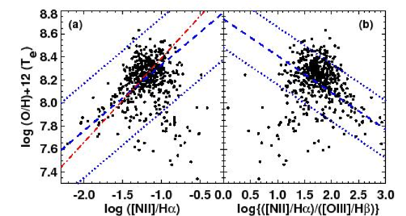
Figure 10.— The observed relationship between the metallicities derived using the T_e  method and (a) the [N II] $\lambda$6584/H$\alpha$ line ratio, and (b) the [O III]/H$\beta$/[N II]/H$\alpha$  ratio. SDSS galaxies with useable [O III] $\lambda 4363$ line fluxes (S/N$>3$) are shown as black filled circles. The PP04 calibration (dashed lines) and 95 percentile lines (dotted lines) are shown for each line ratio. The D02 calibration (red dot-dashed line) is shown for panel (a). A fraction of SDSS-T_e galaxies have T_e metallicities that lie below the 95 percentile line in both the [NII]/H$\alpha$ and [O III]/H$\beta$/[N II]/H$\alpha$ diagrams. These galaxies have high [NII]/H$\alpha$ and [NII]/[OII] ratios, suggesting high (above solar) metallicities. The T_e-method appears to underestimate the metallicity in these galaxies, possibly as a result of temperature gradients or fluctuations that may occur preferentially at high metallicities.

A.4.2 Pilyugin (2005) - P05

Pilyugin (2001) derived an empirical calibration for ${\rm R}_{23}$ based on T_e-metallicities for a sample of H II regions. This calibration has been updated by Pilyugin & Thuan (2005, ; hereafter P05), using a larger sample of H II regions. They perform fits to the relationship between ${\rm R}_{23}$ and T_e-metallicities that includes an excitation parameter $P$ that corrects for the effect of ionization parameter. The resulting calibration has an upper branch calibration that is valid for T_e-based metallicities $12+\log({\rm O/H})$$>8.25$, and a lower branch calibration that is valid for T_e-based metallicities $12+\log({\rm O/H})$$<8.0$. We use the [N II]/[O II] ratio (Figure 8) to discriminate between the upper and lower branches for P05, and we apply the appropriate upper and lower-branch calibrations (equations 22 and 24 in P05):

$$12+\log({\rm O/H})_{upper}=\frac{R_{23}+726.1+842.2P+337.5P^{2}}{85.96+82.76P+43.98P^{2}+1.793R_{23}}$$ (A11)

$$12+\log({\rm O/H})_{lower}=\frac{R_{23}+106.4+106.8P-3.40P^{2}}{17.72+6.60P+6.95P^{2}-0.302R_{23}}$$ (A12)

where $R_{23}=\frac{[{\rm OII}]\,\lambda\lambda 3727,29+[{\rm OIII}]\,\lambda\lambda 4959,5007}{{\rm H}\beta}$, and $P=\frac{[{\rm OIII}]\,\lambda\lambda 4959,5007/{\rm H}\beta}{R_{23}}$ . P05 estimate that the accuracy for reproducing T_e-based metallicities with the P05 calibration is $\sim 0.1$ dex

Because the P05 method was derived using fits to H II regions, we test whether the P05 method is applicable to the relationship between the SDSS T_e metallicities and ${\rm R}_{23}$ in Figure 11. In Figure 11a, we plot all SDSS galaxies in our sample with S/N ratio $>3$ in the [O III] $\lambda 4363$ line. The upper and lower P05 branches are shown for different values of the excitation parameter $P$ (red dot-dashed lines). Several galaxies lie outside the bounds of the P05 lower branch ($12+\log({\rm O/H})$ (Te)$<8.0$).

In Figure 11b, we exclude the galaxies that lie below the lowest 95 percentile line in the PP04 O3N2 calibration (Figure 10b) that are likely to have unreliable T_e metallicities. As we discussed in Section A.4.1, these excluded galaxies have [N II]/H$\alpha$ and [N II]/[O II] ratios that indicate metallicities above solar. We note that the excluded galaxies have excitation parameters between $0.2<P<0.8$, with a mean excitation parameter of $0.46\pm 0.03$. These $P$ values are more consistent with the P05 upper branch (range $0.2<{\rm P}<0.8$, mean $0.64\pm 0.03$) than the P05 lower branch (range $0.6<{\rm P}<1.0$, mean $0.8\pm 0.1$) for our SDSS sample. The T_e method may not be reliable for these galaxies.

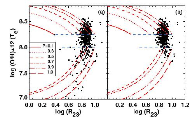
Figure 11.— The observed relationship between the metallicities derived using the T_e  method and the ${\rm R}_{23}$ line ratio for (a) all SDSS galaxies in our sample with measurable (S/N$>3$) [O III] $\lambda 4363$ fluxes, and (b) for the SDSS galaxies in our sample with measurable [O III] $\lambda 4363$ lines that lie above the lowest 95 percentile line in the PP04 O3N2 calibration (Figure 10).

A.5. Combined T_e-strong-line method

A.5.1 Denicolo, Terlevich & Terlevich (2002) - D02

The Denicoló et al. (2002) calibration is based on a fit to the relationship between the T_e metallicities and the [N II]/H$\alpha$ line ratio for $\sim 155$ H II regions. Of these H II regions, $\sim 100$ have metallicities derived using the T_e method, and $55$ H II have metallicities estimated using the theoretical M91 ${\rm R}_{23}$ method, or an empirical method proposed by Díaz & Pérez-Montero (2000) method based on the sulfur lines. The division between H II regions with T_e-based metallicities and those with strong-line metallicities occurs at $12+\log({\rm O/H})$$\sim 8.4$. The D02 calibration is given by a linear least-squares fit:

$$12+\log({\rm O/H})=9.12+0.73\times N2$$ (A13)

where $N2=\log([{\rm NII}]\,\lambda 6584/{\rm H}\alpha)$. D02 estimate that the uncertainty the derived metallicities is $\sim 0.2$ dex.

In Figure 10, we compare the D02 fit (red dot-dashed line) to the [N II]/H$\alpha$-T_erelationship for the SDSS galaxies. The D02 method provides a reasonable fit to the SDSS galaxies, given the large scatter, and is similar to the PP04 N2 curve to within $\sim 0.2$ dex over the metallicity range $7.4<12+\log({\rm O/H})<8.8$.

Appendix B Metallicity Conversions: Worked Examples

Three galaxies have metallicities of $12+\log({\rm O/H})$$=8.3,8.6$, and $9.1$ calculated using three different methods; KK04, PP04, and D02, respectively. To compare these galaxy metallicities with those derived by the SDSS team (Tremonti et al., 2004), we convert the three galaxy metallicities into a metallicity base of T04.

For a galaxy with metallicity $12+\log({\rm O/H})$${}_{KK04}=8.3$, the KK04 metallicity is calculated from the lower ${\rm R}_{23}$ branch (see Section A.2.3). Table 3 gives the coefficients of the polynomial that converts a KK04 metallicity into a T04 base metallicity. Because our KK04 metallicity is from the lower branch, we use the linear relation for the lower branch conversion:

$$[\log{\rm(O/H)}+12]_{T04} = -4.5710+1.53261\times[\log{\rm(O/H)}+12]_{KK04}$$

$$\sim 8.2$$

To convert an original PP04 metallicity ($12+\log({\rm O/H})$${}_{PP04}=8.6$) from O3N2 into a T04 base metallicity, Table 3 gives

$$[\log{\rm(O/H)}+12]_{T04} = -738.1193+258.96730\times[\log{\rm(O/H)}+12]_{PP04}$$

$$-30.057050\times[\log{\rm(O/H)}+12]^{2}_{PP04}$$

$$+1.167937\times[\log{\rm(O/H)}+12]^{3}_{PP04}$$

$$\sim 8.9$$

An original D02 metallicity $12+\log({\rm O/H})$${}_{D02}=9.1$ cannot be converted into a T04 metallicity because this D02 abundance is above the valid range for our conversion from D02 into T04 ($8.05-8.9$).

As a final example, we convert a T04 abundance of $12+\log({\rm O/H})$${}_{T04}=8.3$ into an M91 base metallicity. Note that the valid upper and lower branch ranges overlap for the conversion of T04 into M91, ie. $8.2<\log({\rm O/H})_{T04}<9.2$ (upper branch) and $8.05<\log({\rm O/H})_{T04}<8.4$ (lower branch). At a T04 metallicity between $8.2<\log({\rm O/H})_{T04}<8.3$, the M91 ${\rm R}_{23}$ calibration is reaching a local maximum and is insensitive to metallicity. In this regime, the M91 upper or lower branch should be selected based on the [N II]/[O II] or [N II]/H$\alpha$ ratio (Section A.1). If the log([N II]/H$\alpha$) ratio in our example galaxy is $-0.7$, then Figure 9 indicates that the metallicity is on the ${\rm R}_{23}$ upper branch, and therefore, the conversion from a T04 metallicity of $12+\log({\rm O/H})$${}_{T04}=8.3$ into an M91 base metallicity is

$$[\log{\rm(O/H)}+12]_{M91} = 404.1716-131.53250\times[\log{\rm(O/H)}+12]_{T04}$$

$$+14.49175\times[\log{\rm(O/H)}+12]^{2}_{T04}$$

$$-0.5285842\times[\log{\rm(O/H)}+12]^{3}_{T04}$$

$$\sim 8.6$$

Table 1Comparison of the 10 metallicity calibrations

#	ID	Emission lines	Calibration Class	Reference
1	T04	[OII], H$\beta$, [OIII], H$\alpha$, [NII], [SII]	theoretical	Tremonti et al. (2004)
2	Z94	${\rm R}_{23}$	theoretical	Zaritsky et al. (1994)
3	KK04	${\rm R}_{23}$, [OIII]/[OII]	theoretical	Kobulnicky & Kewley (2004)
4	KD02	[NII]/[OII], ${\rm R}_{23}$, [OIII]/[OII]	theoretical	Kewley & Dopita (2002)
5	M91	${\rm R}_{23}$, [OIII]/[OII]	theoretical	McGaugh (1991)
6	D02	[NII]/H$\alpha$	combined	Denicoló et al. (2002)
7	PP04	[NII]/Ha, [OIII]/H$\beta$	empirical	Pettini & Pagel (2004)
8	PP04	[NII]/Ha	empirical	Pettini & Pagel (2004)
9	P01,P05	${\rm R}_{23}$, [OIII]/[OII]	empirical	Pilyugin (2001); Pilyugin & Thuan (2005)
10	Te	[OIII] $\lambda 4363$, [OIII] $\lambda\lambda 4959,5007$	direct	Aller (1984); Stasińska (2005); Izotov et al. (2006a)

Table 2Robust fits to the MZ relations for the 9 strong-line metallicity calibrations

ID	a	b	c	d	rms residuals
T04	-0.694114	1.30207	0.00271531	-0.00364112	0.12
Z94	72.0142	-20.6826	2.22124	-0.0783089	0.13
KK04	27.7911	-6.94493	0.808097	-0.0301508	0.10
KD02	28.0974	-7.23631	0.850344	-0.0318315	0.10
M91	45.5323	-12.2469	1.32882	-0.0471074	0.11
D02	-8.71120	4.15003	-0.322156	0.00818179	0.08
PP04 O3N2	32.1488	-8.51258	0.976384	-0.0359763	0.10
PP04 N2	23.9049	-5.62784	0.645142	-0.0235065	0.09
P01	91.6457	-25.9355	2.67172	-0.0909689	0.12
P05	41.9463	-10.3253	1.04371	-0.0347747	0.13

Table 3Metallicity Calibration Conversion Constants

ID	KK04	Z94	M91	KD02	T04	D02	PP04 O3N2	PP04 N2
y	(x)	(x)	(x)	(x)	(x)	(x)	(x)	(x)
KK04
x-range		8.4-9.3	8.4-9.1; 8.0-8.25	8.4-9.2; 8.05-8.3	8.3-9.2 ; 8.05-8.4	8.2-8.9 ; 8.05-8.4	8.2-8.9 ; 8.05-8.3	8.2-8.9 ; 8.05-8.3
branch			up; low 0.0.	up; low 0.0.	up; low 0.0.	up; low 0.0.	up; low 0.0.	up; low 0.0.
a		348.1710	-355.2968; 2.0021string	1149.479; 1.0944string	-162.1918; 5.0521string	-1.7278; 6.5483string	389.1568; 6.5339string	211.1405; 5.2218string
b		-117.65370	114.8835; 0.77696string	-389.9349; 0.87842string	57.57935; 0.39887string	1.52612; 0.21508string	-133.79070; 0.21761string	-81.11275; 0.37813string
c		13.502640	-12.09838; string	44.33080; string	-6.533486; string	-0.034389; string	15.59350; string	10.577470; string
d		-0.5130281	0.4258375; string	-1.675994; string	0.249956; string	; string	-0.6020232; string	-0.4510567; string
$\rho_{r}$		0.003	0.007; 0.007 string	0.031; 0.004 string	0.048; 0.029 string	0.065; 0.039 string	0.041; 0.041 string	0.064; 0.038 string
Z94
x-range	8.55-9.2		8.4-9.1	8.4-9.2	8.4-9.2	8.05-8.9	8.05-8.9	8.05-8.8
a	-1112.0910		-868.280	1086.903	11.2595	63.6386	230.9335	40.5515
b	379.11370		291.6262	-366.5700	-1.47641	-13.87785	-76.73906	-8.67461
c	-42.880040		-32.42779	41.41521	0.136681	0.872216	8.711059	0.581691
d	1.6218750		1.206416	-1.554630			-0.3244087
$\rho_{r}$	0.005		0.010	0.040	0.056	0.081	0.052	0.076
M91
x-range	8.25-9.15	8.4-9.2		8.4-9.2 ; 8.1-8.4	8.2-9.2 ; 8.05-8.4	8.2-8.9 ; 8.05-8.4	8.2-8.9; 8.05-8.4	8.2-8.8 ; 8.05-8.3
branch				up; low 0.0.	up; low 0.0.	up; low 0.0.	8.2-8.9; 8.05-8.4	up; low 0.0.
a	-641.2458	393.9855		890.1334; -1.0907	404.1716; 3.0825 string	85.2839; 4.7927 string	267.3936; 2.4196 string	87.3710; 0.7641 string
b	226.42050	-127.86040		-295.90760; 1.12114	-131.53250; 0.61779	-18.63342; 0.40796	-85.20014; 0.70167	-19.39959; 0.90362
c	-26.374200	14.050330		33.004210; string	14.491750; string	1.130870; string	9.219665; string	1.193544; string
d	1.0268860	-0.5109532		-1.2227730; string	-0.5285842; string	; string	-0.3267103; string	; string
$\rho_{r}$	0.008	0.008		0.034; 0.004 string	0.047; 0.044 string	0.071; 0.059 string	0.048; 0.076 string	0.064; 0.070 string
KD02
x-range	8.2-9.2	8.4-9.2	8.5-9.1 ; 8.05-8.3		8.2-9.2 ; 8.05-8.4	8.2-8.9 ; 8.05-8.4	8.2-8.9 ; 8.05-8.3	8.2-8.9 ; 8.05-8.3
branch			up; low 0.0.		up; low 0.0.	up; low 0.0.	up; low 0.0.	up; low 0.0.
a	75.5327	-476.8939	-2127.7470; 1.0007 string		387.2871; 4.1582 string	47.3054; 5.9875 string	159.0567; 5.8961 string	1094.5410; 4.5323 string
b	-23.64323	160.45270	720.35980; 0.88853		-129.69190; 0.49751	-10.06952; 0.27338	-54.18511; 0.28562	-388.67530; 0.45232
c	2.658484	-17.752170	-81.051380; string		14.718030; string	0.649502; string	6.395364; string	46.233760; string
d	-0.0948578	0.6579900	3.0435570; string		-0.5531547; string	; string	-0.2471693; string	-1.8276270; string
$\rho_{r}$	0.038	0.036	0.038; 0.003 string		0.041; 0.039 string	0.048; 0.055 string	0.047; 0.059 string	0.047; 0.054 string
T04
x-range	8.6-9.15 ; 8.2-8.4	8.4-9.2	8.6-9.1 ; 8.05-8.4	8.1-9.2		8.05-8.9	8.05-8.9	8.05-8.9
branch	up; low 0.0.		up; low 0.0.
a	-461.2352; -4.5710 string	-472.8841	-69.7024; -1.0200 string	1.3782		193.9000	-738.1193	-1661.9380
b	158.44840; 1.53261	158.20310	16.68313; 1.13063	0.52591		-64.87895	258.96730	585.17650
c	-17.946070; string	-17.414190	-0.880678; string	0.036003		7.411102	-30.057050	-68.471750
d	0.6828170; string	0.6427315	; string			-0.2756653	1.1679370	2.6766690
$\rho_{r}$	0.060; 0.060 string	0.062	0.062; 0.063 string	0.051		0.072	0.058	0.072
D02
x-range	8.2-9.2	8.4-9.3	8.5-9.1 ; 8.0-8.4	8.05-9.2	8.05-9.2		8.05-8.9	8.05-8.9
branch			up; low 0.0.
a	1202.5280	-114.3143	-121.3958; -1.0361 string	680.5167	253.0031		-1.3992	-629.0499
b	-412.30820	32.79523	28.86410; 1.13468	-235.27350	-87.03697		-5.32702	215.37940
c	47.332730	-2.782591	-1.599613; string	27.345830	10.241880		1.562757	-24.305910
d	-1.8065160	0.0731175	; string	-1.0552390	-0.3984731		-0.0938063	0.9168766
$\rho_{r}$	0.058	0.056	0.061; 0.093 string	0.038	0.044		0.033	0.000
PP04  (O3N2)
x-range	8.2-9.2	8.4-9.3	8.5-9.1 ; 8.05-8.4	8.1-9.2	8.05-9.2	8.05-8.9		8.05-8.8
branch			up; low 0.0.
a	631.2766	52.2389	-65.0991; 2.1063 string	664.8453	230.7820	36.6598		-8.0069
b	-210.02090	-18.67559	15.74995; 0.74427	-225.75330	-75.79752	-7.64786		2.74353
c	23.483050	2.447698	-0.837514; string	25.768880	8.526986	0.508480		-0.093680
d	-0.8704286	-0.1011578	; string	-0.9761368	-0.3162894
$\rho_{r}$	0.050	0.047	0.056; 0.073 string	0.047	0.046	0.045		0.038
PP04  (N2)
x-range	8.2-9.2	8.4-9.3	8.5-9.1 ; 8.05-8.4	8.05-9.2	8.05-9.2	8.05-8.9	8.05-8.9
branch			up; low 0.0.
a	916.7484	656.5128	1334.9130; 3.1447 string	569.4927	319.7570	-444.7831	512.7575
b	-309.54480	-224.11240	-464.86390; 0.61788	-192.51820	-107.13160	165.42600	-180.47540
c	35.051680	25.734220	54.166750; string	21.918360	12.208670	-20.202000	21.415880
d	-1.3188000	-0.9812624	-2.0986640; string	-0.8278840	-0.4606539	0.8249386	-0.8427312
$\rho_{r}$	0.068	0.065	0.071; 0.050 string	0.045	0.051	8.557e-6	0.042

Table 4Residual Metallicity Discrepancy

Base	Mean Residual
ID	Discrepancy (dex)
KK04	0.011
Z94	0.018
M91	0.011
KD02	0.014
T04	0.034
D02	0.034
PP04 O3N2	0.012
PP04 N2	0.021

Table 5Relative median metallicity and rms scatter for the 9 strong-line metallicity calibrations from 30,000 random sets of SDSS galaxies

ID	T04	Z94	KK04	KD02	M91	D02	PP04 (O3N2)	PP04 (N2)	P01	Mean
	med (rms)	med (rms)	med (rms)	med (rms)	med (rms)	med (rms)	med (rms)	med (rms)	med (rms)	rms
T04	$\cdots$	0.006 (0.08)	0.053 (0.09)	0.033 (0.07)	0.036 (0.09)	0.076 (0.10)	0.040 (0.08)	0.053 (0.09)	0.046 (0.14)	0.09
Z94	-0.006 (0.08)	$\cdots$	0.046 (0.05)	0.023 (0.05)	0.024 (0.04)	0.062 (0.09)	0.029 (0.06)	0.042 (0.08)	0.034 (0.11)	0.07
KK04	-0.053 (0.09)	-0.046 (0.05)	$\cdots$	-0.023 (0.05)	-0.014 (0.02)	0.016 (0.06)	-0.017 (0.05)	-0.003 (0.07)	-0.004 (0.09)	0.06
KD02	-0.033 (0.07)	-0.023 (0.05)	0.023 (0.05)	$\cdots$	0.005 (0.05)	0.039 (0.06)	0.006 (0.05)	0.019 (0.05)	0.011 (0.10)	0.06
M91	-0.036 (0.09)	-0.024 (0.04)	0.014 (0.02)	-0.005 (0.05)	$\cdots$	0.031 (0.08)	-0.001 (0.06)	0.009 (0.07)	0.010 (0.08)	0.06
D02	-0.076 (0.10)	-0.062 (0.09)	-0.016 (0.06)	-0.039 (0.06)	-0.031 (0.08)	$\cdots$	-0.033 (0.05)	-0.020 (0.03)	-0.017 (0.11)	0.07
PP04 (O3N2)	-0.040 (0.08)	-0.029 (0.06)	0.017 (0.05)	-0.006 (0.05)	0.001 (0.06)	0.033 (0.05)	$\cdots$	0.014 (0.05)	0.012 (0.12)	0.07
PP04 (N2)	-0.053 (0.09)	-0.042 (0.08)	0.003 (0.07)	-0.019 (0.05)	-0.009 (0.07)	0.020 (0.03)	-0.014 (0.05)	$\cdots$	0.004 (0.11)	0.07
P01	-0.046 (0.14)	-0.034 (0.11)	0.004 (0.09)	-0.011 (0.10)	-0.010 (0.08)	0.017 (0.11)	-0.012 (0.12)	-0.004 (0.11)	$\cdots$	0.11

References

- Afflerbach et al. (1997) Afflerbach, A., Churchwell, E., & Werner, M. W. 1997, ApJ, 478, 190
- Allende Prieto et al. (2001) Allende Prieto, C., Lambert, D. L., & Asplund, M. 2001, ApJ, 556, L63
- Aller (1984) Aller, L. H., ed. 1984, Physics of Thermal Gaseous Nebulae
- Asplund et al. (2004) Asplund, M., Grevesse, N., Sauval, A. J., Allende Prieto, C., & Kiselman, D. 2004, A&A, 417, 751, astro-ph/0312290
- Baldry et al. (2002) Baldry, I. K., et al. 2002, ApJ, 569, 582
- Baldwin et al. (1981) Baldwin, J. A., Phillips, M. M., & Terlevich, R. 1981, PASP, 93, 5
- Bell & de Jong (2000) Bell, E. F., & de Jong, R. S. 2000, MNRAS, 312, 497
- Bell & de Jong (2001) ——. 2001, ApJ, 550, 212
- Boselli et al. (2001) Boselli, A., Gavazzi, G., Donas, J., & Scodeggio, M. 2001, AJ, 121, 753
- Bothun et al. (1984) Bothun, G. D., Romanishin, W., Strom, S. E., & Strom, K. M. 1984, AJ, 89, 1300
- Bresolin (2006a) Bresolin, F. 2006a, ArXiv Astrophysics e-prints, astro-ph/0608410
- Bresolin (2007) ——. 2007, ApJ, 656, 186
- Bresolin et al. (2004) Bresolin, F., Garnett, D. R., & Kennicutt, R. C. 2004, ApJ, 615, 228
- Bresolin et al. (2006) Bresolin, F., Pietrzyński, G., Urbaneja, M. A., Gieren, W., Kudritzki, R.-P., & Venn, K. A. 2006, ApJ, 648, 1007
- Brooks et al. (2007) Brooks, A. M., Governato, F., Booth, C. M., Willman, B., Gardner, J. P., Wadsley, J., Stinson, G., & Quinn, T. 2007, ApJ, 655, L17
- Brown et al. (2006) Brown, W. R., Geller, M. J., Kenyon, S. J., & Kurtz, M. J. 2006, ApJ, 647, in press, astro-ph/0604111
- Bruzual & Charlot (2003) Bruzual, G., & Charlot, S. 2003, MNRAS, 344, 1000
- Calura et al. (2004) Calura, F., Matteucci, F., & Menci, N. 2004, MNRAS, 353, 500
- Cardelli et al. (1989) Cardelli, J. A., Clayton, G. C., & Mathis, J. S. 1989, ApJ, 345, 245
- Carollo & Lilly (2001) Carollo, C. M., & Lilly, S. J. 2001, ApJ, 548, L153
- Davé & Oppenheimer (2007) Davé, R., & Oppenheimer, B. D. 2007, MNRAS, 374, 427
- Davis & Peebles (1983) Davis, M., & Peebles, P. J. E. 1983, ApJ, 267, 465
- De Lucia et al. (2004) De Lucia, G., Kauffmann, G., & White, S. D. M. 2004, MNRAS, 349, 1101
- De Rossi et al. (2006) De Rossi, M. E., Tissera, P. B., & Scannapieco, C. 2006, MNRAS, 374, 323
- Denicoló et al. (2002) Denicoló, G., Terlevich, R., & Terlevich, E. 2002, MNRAS, 330, 69
- Díaz & Pérez-Montero (2000) Díaz, A. I., & Pérez-Montero, E. 2000, MNRAS, 312, 130
- Dopita & Evans (1986) Dopita, M. A., & Evans, I. N. 1986, ApJ, 307, 431
- Dopita et al. (2000) Dopita, M. A., Kewley, L. J., Heisler, C. A., & Sutherland, R. S. 2000, ApJ, 542, 224
- Drory et al. (2004) Drory, N., Bender, R., & Hopp, U. 2004, ApJ, 616, L103
- Edmunds & Pagel (1984) Edmunds, M. G., & Pagel, B. E. J. 1984, MNRAS, 211, 507
- Erb et al. (2006) Erb, D. K., Shapley, A. E., Pettini, M., Steidel, C. C., Reddy, N. A., & Adelberger, K. L. 2006, ApJ, 644, 813
- Ercolano et al. (2007) Ercolano, B., Bastian, N., & Stasinska, G. 2007, MNRAS, 379, 945
- Esteban et al. (2005) Esteban, C., García-Rojas, J., Peimbert, M., Peimbert, A., Ruiz, M. T., Rodríguez, M., & Carigi, L. 2005, ApJ, 618, L95
- Esteban et al. (2004) Esteban, C., Peimbert, M., García-Rojas, J., Ruiz, M. T., Peimbert, A., & Rodríguez, M. 2004, MNRAS, 355, 229
- Esteban et al. (2002) Esteban, C., Peimbert, M., Torres-Peimbert, S., & Rodríguez, M. 2002, ApJ, 581, 241
- Ferland et al. (1998) Ferland, G. J., Korista, K. T., Verner, D. A., Ferguson, J. W., Kingdon, J. B., & Verner, E. M. 1998, PASP, 110, 761
- Finlator & Dave (2007) Finlator, K., & Dave, R. 2007, ArXiv e-prints, 704, 0704.3100
- Fioc & Rocca-Volmerange (1999) Fioc, M., & Rocca-Volmerange, B. 1999, ArXiv Astrophysics e-prints, astro-ph/9912179
- Gallazzi et al. (2005) Gallazzi, A., Charlot, S., Brinchmann, J., White, S. D. M., & Tremonti, C. A. 2005, MNRAS, 362, 41
- García-Rojas et al. (2005) García-Rojas, J., Esteban, C., Peimbert, A., Peimbert, M., Rodríguez, M., & Ruiz, M. T. 2005, MNRAS, 362, 301
- García-Rojas et al. (2006) García-Rojas, J., Esteban, C., Peimbert, M., Costado, M. T., Rodríguez, M., Peimbert, A., & Ruiz, M. T. 2006, MNRAS, 368, 253
- Garnett (2002) Garnett, D. R. 2002, ApJ, 581, 1019
- Garnett et al. (2004a) Garnett, D. R., Edmunds, M. G., Henry, R. B. C., Pagel, B. E. J., & Skillman, E. D. 2004a, AJ, 128, 2772
- Garnett et al. (2004b) Garnett, D. R., Kennicutt, R. C., & Bresolin, F. 2004b, ApJ, 607, L21
- Groves et al. (2006) Groves, B., Dopita, M., & Sutherland, R. 2006, A&A, 458, 405
- Groves et al. (2004) Groves, B. A., Dopita, M. A., & Sutherland, R. S. 2004, ApJS, 153, 9
- Hägele et al. (2006) Hägele, G. F., Pérez-Montero, E., Díaz, Á. I., Terlevich, E., & Terlevich, R. 2006, MNRAS, 372, 293
- Henry & Worthey (1999) Henry, R. B. C., & Worthey, G. 1999, PASP, 111, 919
- Hoyos et al. (2005) Hoyos, C., Koo, D. C., Phillips, A. C., Willmer, C. N. A., & Guhathakurta, P. 2005, ApJ, 635, L21
- Huchra et al. (1983) Huchra, J., Davis, M., Latham, D., & Tonry, J. 1983, ApJS, 52, 89
- Izotov et al. (2006a) Izotov, Y. I., Papaderos, P., Guseva, N. G., Fricke, K. J., & Thuan, T. X. 2006a, A&A, 454, 137
- Izotov et al. (2004) Izotov, Y. I., Stasińska, G., Guseva, N. G., & Thuan, T. X. 2004, A&A, 415, 87
- Izotov et al. (2006b) Izotov, Y. I., Stasińska, G., Meynet, G., Guseva, N. G., & Thuan, T. X. 2006b, A&A, 448, 955
- Jansen et al. (2000a) Jansen, R. A., Fabricant, D., Franx, M., & Caldwell, N. 2000a, ApJS, 126, 331
- Jansen et al. (2000b) Jansen, R. A., Franx, M., Fabricant, D., & Caldwell, N. 2000b, ApJS, 126, 271
- Kannappan & Gawiser (2007) Kannappan, S. J., & Gawiser, E. 2007, ApJ, 657, L5
- Kauffmann et al. (2003) Kauffmann, G. et al. 2003, MNRAS, 341, 33
- Kennicutt et al. (2003) Kennicutt, R. C., Bresolin, F., & Garnett, D. R. 2003, ApJ, 591, 801
- Kewley et al. (2007) Kewley, L. J., Brown, W. R., Geller, M. J., Kenyon, S. J., & Kurtz, M. J. 2007, AJ, 133, 882
- Kewley & Dopita (2002) Kewley, L. J., & Dopita, M. A. 2002, ApJS, 142, 35
- Kewley et al. (2001) Kewley, L. J., Dopita, M. A., Sutherland, R. S., Heisler, C. A., & Trevena, J. 2001, ApJ, 556, 121
- Kewley et al. (2004) Kewley, L. J., Geller, M. J., & Jansen, R. A. 2004, AJ, 127, 2002
- Kewley et al. (2006) Kewley, L. J., Groves, B., Kauffmann, G., & Heckman, T. 2006, MNRAS, 372, 961
- Kewley et al. (2005) Kewley, L. J., Jansen, R. A., & Geller, M. J. 2005, PASP, 117, 227
- Kinman & Davidson (1981) Kinman, T. D., & Davidson, K. 1981, ApJ, 243, 127
- Kniazev et al. (2003) Kniazev, A. Y., Grebel, E. K., Hao, L., Strauss, M. A., Brinkmann, J., & Fukugita, M. 2003, ApJ, 593, L73
- Kniazev et al. (2004) Kniazev, A. Y., Pustilnik, S. A., Grebel, E. K., Lee, H., & Pramskij, A. G. 2004, ApJS, 153, 429
- Kobulnicky et al. (1999) Kobulnicky, H. A., Kennicutt, R. C., & Pizagno, J. L. 1999, ApJ, 514, 544