Metallicities and Physical Conditions in Star-forming Galaxies at $z$ $\sim$ 1.0-1.5

Abstract

We present a study of the mass-metallicity ($M-Z$) relation and H II region physical conditions in a sample of 20 star-forming galaxies at $1.0<z<1.5$ drawn from the DEEP2 Galaxy Redshift Survey. We find a correlation between stellar mass and gas-phase oxygen abundance in the sample and compare it with the one observed among UV-selected $z\sim 2$ star-forming galaxies and local objects from the Sloan Digital Sky Survey (SDSS). This comparison, based on the same empirical abundance indicator, demonstrates that the zero point of the $M-Z$ relationship evolves with redshift, in the sense that galaxies at fixed stellar mass become more metal-rich at lower redshift. Measurements of [O III]/H$\beta$ and [N II]/H$\alpha$ emission-line ratios show that, on average, objects in the DEEP2 $1.0<z<1.5$ sample are significantly offset from the excitation sequence observed in nearby H II regions and SDSS emission-line galaxies. In order to fully understand the causes of this offset, which is also observed in $z\sim 2$ star-forming galaxies, we examine in detail the small fraction of SDSS galaxies that have similar diagnostic ratios to those of the DEEP2 sample. Some of these galaxies indicate evidence for AGN and/or shock activity, which may give rise to their unusual line ratios and contribute to Balmer emission lines at the level of $\sim 20$%. Others indicate no evidence for AGN or shock excitation yet are characterized by higher electron densities and temperatures, and therefore interstellar gas pressures, than typical SDSS star-forming galaxies of similar stellar mass. These anomalous objects also have higher concentrations and star formation rate surface densities, which are directly connected to higher interstellar pressure. Higher star formation rate surface densities, interstellar pressures, and H II region ionization parameters may also be common at high redshift. These effects must be taken into account when using strong-line indicators to understand the evolution of heavy elements in galaxies. When such effects are included, the inferred evolution of the $M-Z$ relation out to $z\sim 2$ is more significant than previous estimates.

1. Introduction

The abundance of heavy elements in the H II regions of galaxies reflects the past history of star formation and the effects of inflows and outflows of gas. A characterization of the evolution of chemical abundances for galaxies of different masses is therefore essential to a complete model of galaxy formation that includes the physics of baryons (De Lucia et al., 2004; Finlator & Dave, 2007). Important observational constraints for such models come from determining the scaling relations at different redshifts among galaxy luminosity, stellar mass, and metallicity, which, for star-forming galaxies, typically consists of the oxygen abundance. However, one of the key challenges is to take the observationally measured quantities, i.e. strong, rest-frame optical emission-line ratios, and connect them with the physical quantity of interest, i.e. oxygen abundance.

Table 1Galaxies Observed with Keck II NIRSPEC

DEEP ID	R.A. (J2000)	Dec. (J2000)	$z_{{\rm H}\alpha}$	$B$	$R$	$I$	$M_{B}$	$U-B$
42044579	02 30 43.46	00 42 43.60	1.0180	23.22	22.97	22.40	-21.20	0.54
22046630	16 50 13.83	35 02 01.78	1.0225	23.64	23.02	22.31	-21.37	0.69
22046748	16 50 14.55	35 02 04.31	1.0241	24.43	23.76	22.90	-20.86	0.86
42044575	02 30 44.85	00 42 51.33	1.0490	23.08	22.94	22.56	-21.06	0.34
42010638	02 29 08.74	00 23 28.40	1.3877	22.93	22.85	22.54	-22.12	0.49
42010637	02 29 08.74	00 23 32.87	1.3882	24.20	23.98	23.72	-20.87	0.44
42021412	02 30 44.55	00 30 50.73	1.3962	24.07	23.74	23.12	-21.91	0.78
42021652	02 30 44.70	00 30 46.19	1.3984	22.97	22.24	21.32	-24.01	1.01

Note. — Units of right ascension are hours, minutes, and seconds, and units of declination are degrees, arcminutes and arcseconds.

In the local universe, Tremonti et al. (2004) have used a sample of $\sim$53,000 emission-line galaxies from the Sloan Digital Sky Survey (SDSS) to investigate the luminosity-metallicity ($L-Z$) and mass-metallicity ($M-Z$) relationships. For this sample, metallicities were estimated on the observed spectra of several strong emission lines, including [O II] $\lambda\lambda$3726, 3729, H$\beta$, [O III]$\lambda\lambda$5007, 4959, H$\alpha$, [N II] $\lambda\lambda$6548, 6584, and [S II] $\lambda\lambda$6717, 6731. At increasing redshifts, as the strong rest-frame optical emission lines shift into the near-IR, metallicities are typically based on smaller subsets of strong emission lines through the use of empirically calibrated abundance indicators (e.g. Pettini & Pagel, 2004; Pagel et al., 1979). Much progress has been made recently in assembling large samples of star-forming galaxies with abundance measurements at both intermediate redshift (Kewley & Dopita, 2002; Savaglio et al., 2005) and at $z>2$ (Erb et al., 2006a). However, we have only begun to gather chemical abundance measurements for galaxies at $z\sim 1-2$ (Maier et al., 2006; Shapley et al., 2005, hereafter Paper I,). In this work, we continue our efforts to fill in the gap of chemical abundance measurements during this important redshift range, which hosts the emergence of the Hubble sequence of disk and elliptical galaxies (Dickinson, 2000), and the buildup of a significant fraction of the stellar mass in the universe (Drory et al., 2005; Dickinson et al., 2003) prior to the decline in global star formation rate (SFR) density (Madau et al., 1996).

Chemical abundances for high-redshift galaxies are commonly estimated using locally calibrated empirical indicators. Yet it is crucial to recognize the fact that a considerable fraction of the $z\sim 1$ and $2$ galaxies with measurements of multiple rest-frame optical emission lines do not follow the local excitation sequence described by nearby H II regions and star-forming galaxies in the diagnostic diagram featuring the [O III] $\lambda$5007/H$\beta$ and [N II] $\lambda$6584/H$\alpha$ emission-line ratios (Paper I; Erb et al., 2006a). On average, the distant galaxies lie offset towards higher [O III] $\lambda$5007/H$\beta$ and [N II] $\lambda$6584/H$\alpha$, relative to local galaxies. As discussed in Paper I and Groves et al. (2006), several causes may account for this offset, in terms of the prevailing physical conditions in the H II regions of high-redshift galaxies. The relevant conditions are H II region electron density, hardness of the ionizing spectrum, ionization parameter, the effects of shock excitation, and contributions from an active galactic nucleus (AGN). It is still unclear which of these are most important for determining the emergent spectra of high- redshift galaxies. Understanding this offset in emission-line ratios is important, not only because it provides evidence that physical conditions in the high redshift universe are different from the local ones, but also because the application of an empirically calibrated abundance indicator to a set of H II regions or star-forming galaxies rests on the assumption that these objects are similar, on average, to those on which the calibration is based.

In this sense, the current work is also motivated by the interpretation of the offset in emission-line ratios among distant galaxies, and an assessment of the reliability of using local abundance calibrations for high-redshift star-forming galaxies. Instead of focusing on high-redshift objects, another approach is to study the properties in a class of nearby objects, which exhibit similar offset behavior on the emission-line diagnostic diagram. Unravelling the relations between the physical conditions and unusual diagnostic line ratios for such objects aids the understanding of high-redshift galaxies. The SDSS, with its rich set of photometric and spectroscopic information, provides an ideal local comparison sample.

In this paper we expand on the analysis presented in Paper I, with an enlarged sample of DEEP2 star-forming galaxies observed with NIRSPEC on the Keck II telescope. The larger number of DEEP2 objects with near-IR observations enforces the conclusions drawn in the previous work. Furthermore, our detailed study of nearby SDSS objects with similar emission-line diagnostic ratios leads to a clearer physical explanation of the observed properties of the DEEP2 galaxies. The DEEP2 sample, near-IR spectroscopic observations, data reduction, and measurements are described in §2. We present the oxygen abundances derived from measurements of [O III], H$\beta$, H$\alpha$, and [N II] emission lines in both individual as well as composite spectra in §3. The mass-metallicity relationship and its evolution through cosmic time are discussed in §4. In §5 we investigate differences in $z\sim 1.0-1.5$ H II region physical conditions with respect to local samples by examining nearby SDSS galaxies with similar emission-line diagnostic ratios. Finally, we summarize our main conclusions in §6. A cosmology with $\Omega_{m}=0.3$, $\Omega_{\Lambda}=0.7$, and $h=0.7$ is assumed throughout.

2. DEEP2 Sample, Observations, and Data Reduction

2.1. DEEP2 Target Sample and Near-IR Spectroscopy

The high-redshift galaxies presented in this paper are drawn from the DEEP2 Galaxy Redshift Survey (hereafter DEEP2; Davis et al., 2003; Faber et al., 2007), which contains $>30,000$ galaxies with high-confidence redshifts at $0.7\leq z\leq 1.5$ down to a limiting magnitude of $R_{AB}=24.1$. The motivation for our follow-up near-infrared spectroscopic program, along with detailed descriptions of the sample selection, optical and near-IR photometry, and spectroscopy are presented in Paper I. Only a brief overview is given here.

The new sample contains four galaxies at $z\sim 1.0$ and four galaxies at $z\sim 1.4$, which, in combination with the pilot program presented in Paper I, leads to a sample of 20 galaxies in total. These galaxies are located in fields 2, 3, and 4 of the DEEP2 survey, at 16, 23, and 2 hr right ascension, respectively. To probe chemical abundances and H II region physical conditions, observations of several strong H II region emission lines are required, ideally at least [O II], H$\beta$, [O III], H$\alpha$, and [N II]. At $z\geq 0.85$, however, the only strong H II region emission feature contained in the DEEP2 DEIMOS spectroscopic data is the [O II] doublet. Therefore, near-IR spectroscopy is needed to measure longer wavelength H II region emission lines at $z\geq 1$. We target two narrow redshift windows within the larger DEEP2 redshift distribution: $0.96\leq z\leq 1.05$ and $1.36\leq z\leq 1.50$, within which it is possible to measure the full set of H$\beta$, [O III], H$\alpha$, and [N II], in spite of the bright sky lines and strong atmospheric absorption in the near-IR.

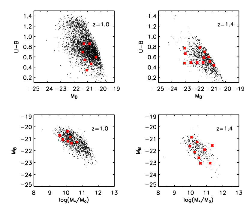
Figure 1.— DEEP2 color-magnitude and magnitude-stellar mass diagrams. The rest-frame $(U-B)$ vs. $M_{B}$ color-magnitude diagrams (top) and the $M_{B}$ vs. stellar mass diagrams (bottom) are for DEEP2 galaxies at $0.96\leq z\leq 1.05$ (left) and $1.36\leq z\leq 1.50$ (right). In each plot, DEEP2 galaxies from both the pilot sample presented in Paper I as well as objects with new NIRSPEC observations are indicated with red squares. As shown here, all NIRSPEC targets were drawn from the “blue cloud” of the color bimodality. .

The absolute $B$ magnitude, $M_{B}$, and stellar mass estimates are given in Tables 1 and 2 for the new objects and plotted as red squares in the lower panels of Figure 1, together with the data for the pilot sample. For all the objects, we use the $M_{B}$ values from Willmer et al. (2006) based on optical data alone and confirm their good agreement with estimates based on fits to the $BRIK_{S}$ SEDs that span through rest-frame $J$ ($I$) band for the objects at $z\sim 1.0$ ($z\sim 1.4$). Stellar masses for the objects in our sample are derived with $K_{S}$-band photometry, following the procedure outlined in Bundy et al. (2005), which assumes a Chabrier (2003) stellar initial mass function (IMF). As discussed in detail in Paper I, the Bundy et al. (2005) stellar mass modelling technique agrees well with that used by Kauffmann et al. (2003b) for SDSS galaxies, based on both spectral features and broadband photometry. Stellar masses for galaxies in the pilot sample have been updated to reflect both the most current DEEP2 near-IR photometric catalog, and population synthesis models limiting the stellar population age to be younger than the age of the Universe at $z\sim 1$. Thus, in a few cases, the stellar masses differ slightly from those presented in Table (2) of Paper I. As shown in the lower panels of Figure (1), the $z\sim 1.4$ galaxies in our sample span the full range of absolute $B$ luminosities in the DEEP2 survey, from $M_{B}\sim$ -20 to -23, while the smaller set of $z\sim 1.0$ galaxies happens to cover the faint end of the luminosity function. Galaxies in both redshift intervals cover more than an order of magnitude in stellar mass and therefore should be able to probe an interesting dynamic range. Since our goal was to study the emission-line properties of galaxies, all objects in our sample lie in the blue component of the observed $(U-B)$ color bimodality in the DEEP2 survey, as shown in the upper panels of Figure 1.

Table 2Emission Lines and Physical Quantities.

						12 + log(O/H)
DEEP ID	zHα	FHβ	F[OIII]λ5007	FHα	F[NII]λ6584	N2	O3N2	$L_{H\alpha}$	SFRHα	log$(M_{\ast}/M_{\odot})$
42044579	1.0180	2.4$\pm$0.4	5.4$\pm$0.3	12.1$\pm$0.3	2.8$\pm$0.3	8.54$\pm$0.18	8.41$\pm$0.14	0.7	3	10.26$\pm$0.15
22046630	1.0225	3.7$\pm$0.5	8.7$\pm$0.4	15.2$\pm$0.3	1.8$\pm$0.3	8.37$\pm$0.18	8.32$\pm$0.14	0.8	3	10.29$\pm$0.16
22046748	1.0241	2.2$\pm$0.4	6.4$\pm$0.3	9.6$\pm$0.2	2.3$\pm$0.2	8.55$\pm$0.18	8.39$\pm$0.14	0.5	2	10.28$\pm$0.10
42044575	1.0490	7.7$\pm$0.7	22.9$\pm$0.3	23.6$\pm$0.3	3.6$\pm$0.3	8.43$\pm$0.18	8.32$\pm$0.14	1.4	6	9.74$\pm$0.06
42010638	1.3877	3.8$\pm$0.9	17.3$\pm$0.4	16.6$\pm$0.5	2.8$\pm$0.5	8.46$\pm$0.19	8.27$\pm$0.15	2.0	9	10.21$\pm$0.06
42010637	1.3882	3.3$\pm$0.9	3.7$\pm$0.3	6.4$\pm$0.4	2.9$\pm$0.4	8.70$\pm$0.18	8.60$\pm$0.15	0.8	4	9.96$\pm$0.12
42021412	1.3962	7.1$\pm$0.8	$>$ 2.0	12.7$\pm$0.3	2.9$\pm$0.3	8.54$\pm$0.18	$<$ 8.70	1.5	7	10.89$\pm$0.13
42021652	1.3984	4.6$\pm$0.5	9.7$\pm$0.5	9.5$\pm$0.3	1.2$\pm$0.3	8.38$\pm$0.19	8.33$\pm$0.15	1.1	5	…

The near-IR spectra were obtained on 2005 September 17 and 18 with the NIRSPEC spectrograph (McLean et al., 1998) on the Keck II telescope. Over the range of redshifts of the galaxies presented here, two filter setups are required to measure the full set of H$\beta$, [O III], H$\alpha$, and [N II]. For objects at $z\sim 1.4$, the NIRSPEC 5 filter (similar to $H$ band) is used to observe H$\alpha$ and [N II], whereas the NIRSPEC 3 filter (similar to $J$ band) is used for H$\beta$ and [O III]. For objects at $z\sim 1.0$, the NIRSPEC 3 filter is used to observe H$\alpha$ and [N II], whereas the NIRSPEC 1 filter ($\Delta\lambda=$ 0.95-1.10 $\mu$m) is used for H$\beta$ and [O III]. All targets were observed for 3$\times$900 s in each filter with a 0.76${}^{{}^{\prime\prime}}$$\times$42${}^{{}^{\prime\prime}}$ long slit. The spectral resolution determined from sky lines is $\sim 10{\rm\AA}$ for all four NIRSPEC filters used here. Photometric conditions and seeing were variable throughout both nights, with seeing ranging from 0.5${}^{{}^{\prime\prime}}$ to 0.7${}^{{}^{\prime\prime}}$ in the near-IR. In order to enhance the long-slit observing efficiency, we targeted two galaxies simultaneously by placing them both on the slit.

We observed a total of 10 DEEP2 galaxies, successfully measuring the full set of H$\beta$, [O III], H$\alpha$, and [N II] for eight out of 10. For the remaining pair, we only detected H$\alpha$ in the $H$ band, but no H$\beta$ nor [O III] in the $J$-band exposures, in which the background in between sky lines was characterized by a significantly higher level of continuum than usual. This anomalous background is likely due to an increased contribution from clouds, which may have affected both $H$- and $J$-band observations of the pair. Since a clear measurement was not obtained for these two objects, due to variable weather conditions, we exclude them from our study. The object, 42021652, has a double morphology, with one component dominated by emission lines with a weak continuum, and another component dominated by strong continuum, with only weak emission lines at roughly the same redshift. The separation between the two components on the sky is $\sim$0.9${}^{{}^{\prime\prime}}$, which corresponds to $\sim$8 kpc at $z=1.3984$, perhaps indicative of a merger event. This interpretation is supported by the small velocity difference of $\Delta v\sim 125$ km s^-1 between the two components. We measure line fluxes for the component dominated by emission lines, since it provides a more robust estimate of line ratios. Deblended optical and near-infrared magnitudes would be required to obtain robust stellar masses for the individual components. However, in the DEEP2 photometry the two components were counted as one source since they are too close to be deblended and the stellar mass has contribution from both of them. For now, we only include flux measurements of the emission-line component for the diagnostic-line-ratio analysis but do not include this object in the mass-metallicity studies. A summary of the observations including target coordinates, redshifts, and optical and near-IR photometry is given in Table 1.

2.2. Data Reduction and Optimal Background Subtraction

Data reduction was performed with a similar procedure to the one described in Paper I and Erb et al. (2003), with the exception of an improved background subtraction method applied to the two-dimensional galaxy spectral images (Kelson, 2003; Becker, 2006, private communication). In the custom NIRSPEC long-slit reduction package written by D. G. Becker (2006, private communication), optimal background subtraction is performed on the unrectified science frames. First, a transformation is calculated between CCD ($x$, $y$) coordinates and those of slit position and wavelength, using the wavelength-dependent traces of bright standard stars and the spatially dependent curves of bright sky lines. Then a two-dimensional model of the sky background is constructed as a function of slit position and wavelength, using a low-order polynomial in the slit-position dimension, and a $b$-spline function in the wavelength dimension. This two-dimensional model is iteratively fit in the differenced frame of adjacent science exposures and subtracted from the unrectified data. After background subtraction, cosmic rays were removed from each exposure, which was then rotated, cut out along the slit, and rectified. Finally, all background-subtracted, rectified exposures of a given science target were combined in two dimensions. This new approach to reducing NIRSPEC spectra results in fewer artifacts around bright sky lines and cosmic rays, which are commonly introduced when rectification is performed before sky subtraction and cosmic-ray zapping. One-dimensional spectra, along with error spectra, were then extracted and flux- calibrated using A-star observations, according to the procedure described in Paper I and Erb et al. (2003).

2.3. Measurements and Physical Quantities

Figure 2.— NIRSPEC spectra of DEEP2 galaxies in our new sample at $z\sim 1.0$. H$\beta$ and [O III] are observed in the NIRSPEC 1 filter, with H$\alpha$ and [N II] in the NIRSPEC 3 filter (similar to the $J$ band). The 1 $\sigma$ error spectra are shown as dotted lines, offset vertically by $-5\times 10^{-18}$ ergs s^-1 cm^-2 Å^-1 for clarity.

Figure 3.— NIRSPEC spectra of DEEP2 galaxies in our new sample at $z\sim 1.4$. H$\beta$ and [O III] are observed in the NIRSPEC 3 filter, with H$\alpha$ and [N II] in the NIRSPEC 5 filter (similar to the $H$ band). The 1 $\sigma$ error spectra are shown as dotted lines, offset vertically by $-5\times 10^{-18}$ ergs s^-1 cm^-2 Å^-1 for clarity.

One-dimensional, flux-calibrated NIRSPEC spectra along with the 1 $\sigma$ error spectra of galaxies in our new sample are shown in Figures 2 and 3. Emission-line fluxes and uncertainties measured from the one-dimensional spectra are given in Table 2. H$\alpha$ and [N II] $\lambda$6584 emission-line fluxes were determined by first fitting a Gaussian profile to the H$\alpha$ feature to obtain the redshift and FWHM, and using these values to constrain the fit to the [N II] emission line. This method is based on the assumption that the H$\alpha$ and [N II] lines have exactly the same redshift and FWHM, with the H$\alpha$ line having a higher signal-to-noise ratio (S/N). For most of the objects in our sample, the [N II] $\lambda$6548 line was too faint to measure. [O III] $\lambda$5007 and H$\beta$ fluxes were determined with independent fits. In most cases, redshifts from H$\alpha$, [O III] $\lambda$5007, and H$\beta$ agree to within $\Delta z=0.0004$ ($\Delta v=50-60$ km s^-1 at $z=1.0-1.4$). For the object 42021412, [O III] $\lambda$5007 lies on top of a bright sky line, and only a lower limit is given.

SFRs inferred from H$\alpha$ luminosities using the calibration of Kennicutt (1998) are shown in Table (2). The results have been converted from the Salpeter IMF used by Kennicutt (1998) to a Chabrier (2003) IMF by dividing the results by a factor of $1.8$. In our whole sample of 20 galaxies, the H$\alpha$ fluxes range from $5.6\times 10^{-17}$ to $2.4\times 10^{-16}$ erg s^-1 cm^-2. The mean H$\alpha$ flux for the sample at $z\sim 1.0$ ($z\sim 1.4$) is $1.3\times 10^{-16}$ ($1.2\times 10^{-16}$), corresponding to a star formation rate of 3 (6) $M_{\odot}$ yr^-1, uncorrected for dust extinction or aperture effects, which may amount to a factor of $2$ difference (Erb et al., 2006b). Note that these characteristic H$\alpha$ star formation rates, after being corrected for aperture effects, would be significantly higher than those of local galaxies in the SDSS sample of Tremonti et al. (2004) and the $\langle z\rangle=0.4$ TKRS subsample of Kobulnicky & Kewley (2004), even before correction for dust extinction. We also note that the mean specific SFR for both $z\sim 1.0$ and $z\sim 1.4$ samples is $\log((SFR/M_{\star})\mbox{ yr}^{-1})=-9.7$.

As discussed in Paper I, absolute line flux measurements suffer from several sources of systematic error, which can amount to at least a $\sim 25\%$ uncertainty (Erb et al., 2003). This level of uncertainty is present even under photometric conditions, which may not have applied through the full extent of our observations. For the remainder of the discussion we therefore focus on the measured line ratios, [N II] $\lambda$6584/H$\alpha$ and [O III] $\lambda$5007/H$\beta$, which are not only unaffected by uncertainties in flux calibration and other systematics but also relatively free from the effects of dust extinction, due to the close wavelength spacing of the lines in each ratio. Hereafter, we use “[N II]/H$\alpha$” to refer to the measured emission-line flux ratio between [N II] $\lambda$6584 and H$\alpha$, and “[O III]/H$\beta$” for that between [O III] $\lambda$5007 and H$\beta$.

3. The Oxygen Abundance

H II region metallicity is an important probe of galaxy formation and evolution, as it represents the integrated products of past star formation, modulated by the inflow and outflow of gas. Oxygen abundance is often used as a proxy for metallicity since oxygen makes up about half of the metal content of the interstellar medium and exhibits strong emission lines from multiple ionization states in the rest-frame optical that are easy to measure. For comparison, we use the solar oxygen abundance expressed as 12 + log(O/H) = 8.66 (Allende Prieto et al., 2002; Asplund et al., 2004).

The most robust way to estimate the oxygen abundance is the so-called direct $T_{e}$ method, based on the measurement of the temperature-sensitive ratio of auroral and nebular emission lines. However, in distant galaxies the auroral lines are almost always undetectable (but see Hoyos et al., 2005; Kakazu et al., 2007) since they become extremely weak at metallicities above $\sim$0.5 solar. Even at lower metallicities, the auroral lines are typically beyond the reach of the low S/N typical of the spectra of distant galaxies. For distant star-forming galaxies, therefore, measuring strong emission-line ratios is the only viable way of obtaining the H II region gas-phase oxygen abundance (Kobulnicky et al., 1999; Pettini et al., 2001).

Given our NIRSPEC data set, and our desire to avoid the systematic uncertainties entailed in adding [O II] line fluxes obtained with the DEIMOS spectrograph (without real-time flux-calibration) to [O III] fluxes obtained with NIRSPEC, we focus on two strong-line ratios as indicators for the oxygen abundance: N2$\equiv$ log([N II]/H$\alpha$) and O3N2$\equiv$ log{([O III]/H$\beta$)/([N II]/H$\alpha$)}. These indicators have been calibrated by Pettini & Pagel (2004) using local H II regions, most of which have direct $T_{e}$ abundance determinations. The sensitivity of the indicators to oxygen abundance, as well as their limitations, have been discussed in Pettini & Pagel (2004) and Paper I. Absolute estimates of metal abundances are quite uncertain, as abundances determined with different indicators or with different calibrations of the same indicator may have substantial biases or discrepancies (e.g. Kennicutt et al., 2003; Kobulnicky & Kewley, 2004). We therefore emphasize relative abundances determined with the same method, using the same calibration.

The N2 indicator, pointed out by several works (Storchi-Bergmann et al., 1994; Raimann et al., 2000; Denicoló et al., 2002), is related to the oxygen abundance via

$${\rm 12+log(O/H)=8.90+0.57\times}{\rm N2},$$ (1)

which is valid for ${\rm 7.50<12+log(O/H)<8.75}$, with a 1 $\sigma$ scatter of $\pm 0.18$ dex (Pettini & Pagel, 2004). It has been used by Erb et al. (2006a) to estimate oxygen abundances for UV-selected $z\sim 2$ galaxies. Note that the N2 indicator is not sensitive to increasing oxygen abundance above roughly solar metallicity, as shown with photoionization models (Kewley & Dopita, 2002). Thus, for a subset of 12 galaxies in our sample with measurements of the full set of H$\beta$, [O III], H$\alpha$, and [N II], we also use the O3N2 indicator introduced by Alloin et al. (1979), which is expected to be particularly useful at solar and super-solar metallicities where [N II] saturates but the strength of [O III] continues to decrease with increasing metallicity. Using the same calibration sample, Pettini & Pagel (2004) show that O3N2 is related to the oxygen abundance via

$${\rm 12+log(O/H)=8.73-0.32\times}{\rm O3N2},$$ (2)

which is valid for ${\rm 8.12<12+log(O/H)<9.05}$, with a 1 $\sigma$ scatter of $\pm 0.14$ dex. Table 2 lists oxygen abundances derived using these two indicators. The errors on the oxygen abundances are dominated by the systematic uncertainties in the calibrations of the indicators.

3.1. Composite Spectra

Figure 4.— Composite NIRSPEC spectra of the 18 $z\sim 1.0-1.5$ galaxies with both stellar mass estimation as well as [N II] and H$\alpha$ measurement in our sample, divided separately at $z\sim 1.0$ and $z\sim 1.4$. The 1 $\sigma$ error spectra are shown as dotted lines, offset vertically by $-3\times 10^{-18}$ ergs s^-1 cm^-2 Å^-1 for clarity. The spectra are labeled with the mean stellar mass from each bin, and the H$\alpha$, [N II] and [S II] lines are marked by dashed lines. Note that the spectra near the density-sensitive [S II] lines are very noisy, due to the large dispersion of the flux per count from near-IR standard star calibration, caused by low efficiency near the filter edge.

Figure 5.— Composite NIRSPEC spectra of the 12 $z\sim 1-1.5$ galaxies with both stellar mass estimation as well as all-four-line measurement in our sample, divided separately at $z\sim 1.0$ and $z\sim 1.4$. The 1 $\sigma$ error spectra are shown as dotted lines, offset vertically by $-3\times 10^{-18}$ ergs s^-1 cm^-2 Å^-1 for clarity. The spectra are labeled with the mean stellar mass from each bin, and the H$\beta$, [O III], H$\alpha$, [N II] and [S II] lines are marked by dashed lines.

Relative, average abundances determined from composite spectra can be more accurately determined than those from individual spectra. As discussed by Erb et al. (2006a), making a composite spectrum not only reduces the uncertainties associated with the strong-line calibration by a factor $N^{1/2}$, where $N$ is the number of objects included in the composite spectrum, but also enhances the spectrum S/N since sky lines generally lie at different wavelengths for spectra at different redshifts. In addition, one of our goals is to determine the average properties of subgroups of galaxies in our sample. For the subset of 18 galaxies in our sample with H$\alpha$ and [N II] measurements, as well as stellar mass estimates, we divide the sample into four bins by stellar mass, with two bins at $z\sim 1.0$ and two bins at $z\sim 1.4$. For the subset of 12 galaxies with measurements of not only H$\alpha$ and [N II], but also H$\beta$ and [O III], we also divide the sample into four bins by stellar mass with two bins each at $z\sim 1.0$ and at $z\sim 1.4$.

To make the composite spectra, we first shift the individual one-dimensional flux-calibrated spectra into the rest frame and then combine them by generating the median spectrum, which preserves the relative fluxes of the emission features (Vanden Berk et al., 2001). We use N2 and N2+O3 composite spectra to refer to the composites with H$\alpha$ and [N II], and those with all four lines, respectively. The N2 and N2+O3 composite spectra, labelled with mean stellar mass in each bin, are shown in Figures 4 and 5. The corresponding emission-line flux ratios along with uncertainties measured from the composite spectra, as well as the inferred oxygen abundances, are listed in Tables 3 and 4. The listed errors in 12 + log(O/H) include the uncertainties from the propagation of emission-line flux measurements, as well as the systematic scatter from the strong-line calibration. As shown in paper I, the systematic discrepancies between the N2- and O3N2-based abundances are mainly due to the fact that, on average, DEEP2 galaxies are offset from the excitation sequence formed by local H II regions and star-forming galaxies. We discuss this issue in detail in §5.

4. The Mass-Metallicity Relation

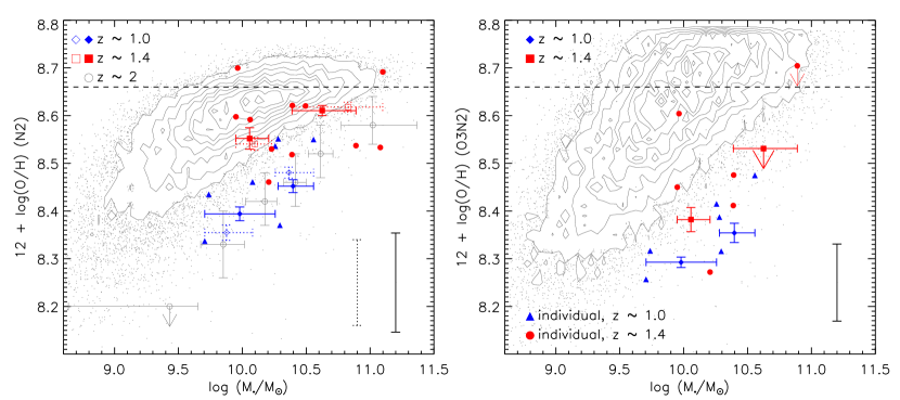
Figure 6.— Mass-metallicity relation observed at $z\sim 1.0$ and $z\sim 1.4$. In the left panel, metallicities are inferred from the N2 indicator, while the right panel shows metallicities estimated from the O3N2 indicator. In both plots, open (filled) diamonds and squares are used for N2 (N2+O3) composite spectra at $z\sim 1.0$ and $z\sim 1.4$, respectively (see section 3.1). Errors show the uncertainties propagated from the strong-line ratio measurement, while the systematic uncertainties from the strong-line method calibration (Pettini & Pagel, 2004) are shown in the lower right corner of each plot as dotted (solid) error bars for N2 (N2+O3) composite spectra. The systematic uncertainties from the calibration are reduced by a factor $N^{1/2}$, where $N$ is the number of individual spectra included in each composite. For stellar masses, the horizontal bars give the mass range in each bin. Data points for individual objects are shown as filled triangles and circles for $z\sim 1.0$ and $z\sim 1.4$, respectively. Associated error bars are listed in Table 2 in both this paper and in Paper I. For comparison, metallicities as a function of stellar mass are also shown, for both local SDSS galaxies (grey contours and dots) and the Erb et al. (2006a) $z\sim 2$ sample (grey open circles, left panel). Note that here and throughout, we use contours and dots to show SDSS objects. On each such applicable plot, SDSS data points were mapped onto 10 evenly spaced levels according to number density, where objects on the lowest level are denoted by dots while other levels are presented by contours. Solar metallicity is marked with a horizontal dashed line. It can be seen that the N2 indicator saturates near the solar abundance.

The redshift evolution of the luminosity-metallicity and mass-metallicity relations provides important constraints on models of galaxy evolution. A correlation between gas-phase metallicity and stellar mass can be explained by either the tendency of lower mass galaxies to have larger gas fractions and lower star formation efficiencies (McGaugh & de Blok, 1997; Bell & de Jong, 2000; Kobulnicky et al., 2003), or the preferential loss of metals from galaxies with shallow potential wells by galactic-scale winds (Larson, 1974). In the local universe, strong correlations between rest-frame optical luminosity and the degree of chemical enrichment have been observed in both star-forming and early-type galaxies (Garnett & Shields, 1987; Brodie & Huchra, 1991; Tremonti et al., 2004). The correlation has also been observed in intermediate- and high- redshift samples (Kobulnicky et al., 2003; Lilly et al., 2003; Kobulnicky & Kewley, 2004; Erb et al., 2006a), although caution must be taken when comparing samples with metallicities determined from different methods. Physically, the correlation between stellar mass and metallicity is more fundamental than that between luminosity and metallicity (Paper I; Tremonti et al., 2004; Erb et al., 2006a). We therefore focus on the mass-metallicity relation in the following discussion.

The left panel of Figure 6 shows the average metallicity of the galaxies in each mass bin determined from the N2 composite spectra plotted against their average stellar mass at $z\sim 1.0$ (open diamonds) and at $z\sim 1.4$ (open squares). Although our sample is still small, we do see evidence for mass-metallicity relations at both $z\sim 1.0$ and $z\sim 1.4$. These trends are also present when we examine the metallicities and stellar masses for individual objects, which are plotted in the figure as well. For comparison, the local SDSS galaxies discussed by Tremonti et al. (2004) are denoted by contours and dots and the $z\sim 2$ Erb et al. (2006a) sample as open circles. Metallicities for SDSS galaxies were calculated using the same strong-line indicator that was applied to the DEEP2 galaxies and not the Bayesian O/H estimate from Tremonti et al. (2004).

At fixed stellar mass, the metallicities of our $z\sim 1.0-1.5$ sample as a whole are lower than those of local galaxies yet higher than those of the $z\sim 2$ sample. However, there is evidence for a reverse trend between the subsets of our sample at $z\sim 1.0$ and at $z\sim 1.4$. In Paper I, this difference was attributed to the fact that the $z\sim 1.0$ sample was on average fainter and less massive than the $z\sim 1.4$ sample. With a larger sample, however, we find that the higher mass $z\sim 1.0$ bin does have lower metallicity than the lower mass $z\sim 1.4$ bin. Differences in outflow or inflow rate of unenriched gas at $z\sim 1.0$ and at $z\sim 1.4$ could give rise to this trend. However, the interval in cosmic time between $z\sim 1.4$ and $1.0$ is small enough that typical gas inflow rates at fixed stellar mass, and the corresponding star formation and outflow rates, will not significantly evolve. Therefore, this explanation is not a likely cause of the reverse trend. A different average degree of dust reddening at $z\sim 1.0$ and at $z\sim 1.4$ is also not a likely cause, since the N2 indicator is based on emission lines with very close spacing in wavelength. On the other hand, if the $z\sim 1.0$ galaxies have systematically different physical conditions or less significant contributions from AGN activity relative to the $z\sim 1.4$ objects, metallicities estimated with the same calibration would be systematically biased between the two samples in such a way to produce the observed trend. As discussed in §5, we propose that the most likely cause for the reverse trend is this difference in H II region physical conditions. Since the systematic uncertainty from strong-line calibration is large, and our sample is still too small to draw any solid conclusion, it will become feasible to clarify this issue only when a statistically large enough sample is assembled, and both the high- and low- mass ends are spanned at $z\sim 1.0$ as well as at $z\sim 1.4$.

We also plot the mass-metallicity relation from the N2+O3 composite spectra in Figure 6, where the left panel shows metallicities determined from the N2 indicator, while the right panel shows those determined from the O3N2 indicator, at both $z\sim 1.0$ (filled diamonds) and $z\sim 1.4$ (filled squares). The O3N2-based abundances are systematically lower than those based on N2. As suggested in Paper I and discussed in detail in §5, these systematic discrepancies between N2- and O3N2-based abundances are due to the fact that DEEP2 galaxies depart from the local H II region excitation sequence. In addition, the reverse trend between $z\sim 1.0$ and $1.4$ in metallicity estimated from O3N2 is much less significant than the one in metallicity estimated from N2. We return to this issue as well in §5. Despite these discrepancies, the overall correlation between average stellar mass and metallicity observed among the N2 composite spectra is still present for the N2+O3 spectra. This is evidence that the correlation is insensitive to the spectrum of any particular object, as it is robust to analyses using different binning schemes. At the lower mass end ($M_{\star}\sim 8\times 10^{9}$ $M_{\sun}$), the average metallicity of $z\sim 1.0-1.5$ galaxies based on N2 is at least 0.22 dex lower than the local typical value. Since the N2 indicator saturates near solar abundance, as discussed in Erb et al. (2006a), it is difficult to determine the true metallicity offset between two samples at different redshifts using this indicator. We can also determine the offset from the O3N2-based abundances, particularly near the solar abundance. Based on O3N2 abundances, the metallicity offset between our DEEP2 objects and the local SDSS sample is at least 0.21 dex at the high-mass end ($M_{\star}\sim 5\times 10^{10}$ $M_{\sun}$). However, as we discuss in §5, these estimates based on strong-line indicators may still be subject to systematic uncertainties from using the calibration of H II regions with significantly different physical properties.

Table 3Oxygen Abundances from N2 composite spectra.

Bin	N	$\langle{\rm z}_{{\rm H}\alpha}\rangle$	log$(M_{\ast}/M_{\odot})$	N2	12 + log(O/H)
1	3	1.0375	$9.88^{+0.10}_{-0.13}$	-0.96$\pm$0.03	8.35$\pm$0.11
2	4	1.0207	$10.37^{+0.05}_{-0.06}$	-0.74$\pm$0.02	8.48$\pm$0.09
3	5	1.3930	$10.10^{+0.06}_{-0.06}$	-0.63$\pm$0.02	8.54$\pm$0.09
4	6	1.3903	$10.83^{+0.05}_{-0.05}$	-0.49$\pm$0.02	8.62$\pm$0.08

Table 4Oxygen Abundances from N2+O3 composite spectra.

Bin	N	$\langle{\rm z}_{{\rm H}\alpha}\rangle$	log$(M_{\ast}/M_{\odot})$	N2	O3N2	[12 + log(O/H)]N2	[12 + log(O/H)]O3N2
1	3	1.0372	$9.98^{+0.09}_{-0.11}$	-0.89$\pm$0.03	1.37$\pm$0.03	8.39$\pm$0.10	8.29$\pm$0.08
2	3	1.0216	$10.40^{+0.06}_{-0.06}$	-0.79$\pm$0.02	1.17$\pm$0.06	8.45$\pm$0.10	8.35$\pm$0.08
3	3	1.3923	$10.06^{+0.06}_{-0.06}$	-0.61$\pm$0.04	1.09$\pm$0.08	8.55$\pm$0.11	8.38$\pm$0.08
4	3	1.3858	$10.63^{+0.07}_{-0.09}$	-0.51$\pm$0.02	$>$ 0.62	8.61$\pm$0.10	$<$ 8.53

5. The Offset in Diagnostic Line Ratios of High-Redshift Galaxies

5.1. Emission-Line Diagnostics

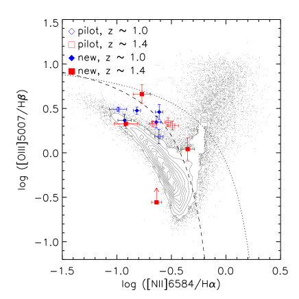
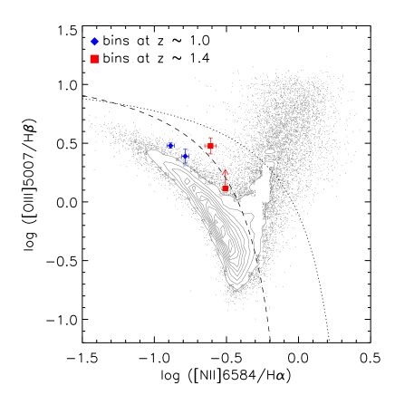
Figure 7.— H II region log[N II]/H$\alpha$ vs. log[O III]/H$\beta$ diagram. On the left, the $z\sim$1.0-1.5 DEEP2 galaxies are shown as indicated on the plot. The right panel shows the average diagnostic line ratios from the composite spectra of DEEP2 objects. Note the bin with the highest [N II]/H$\alpha$ value only has a lower limit on [O III]/H$\beta$ because it includes the object 42021412. SDSS emission-line galaxies that satisfy the criteria described in §5.2 are shown as grey contours and dots. The dashed line is an empirical demarcation from Ka03 based on the SDSS galaxies, whereas the dotted line is the theoretical limit for star-forming galaxies from Ke01. Nearby star-forming galaxies and H II regions form a well-defined excitation sequence of photoionization by massive stars, below and to the left of these curves. The $z\sim 1.0-1.5$ DEEP2 objects on average are offset from this excitation sequence, with objects at $z\sim$1.4 more offset than those at $z\sim$1.0.

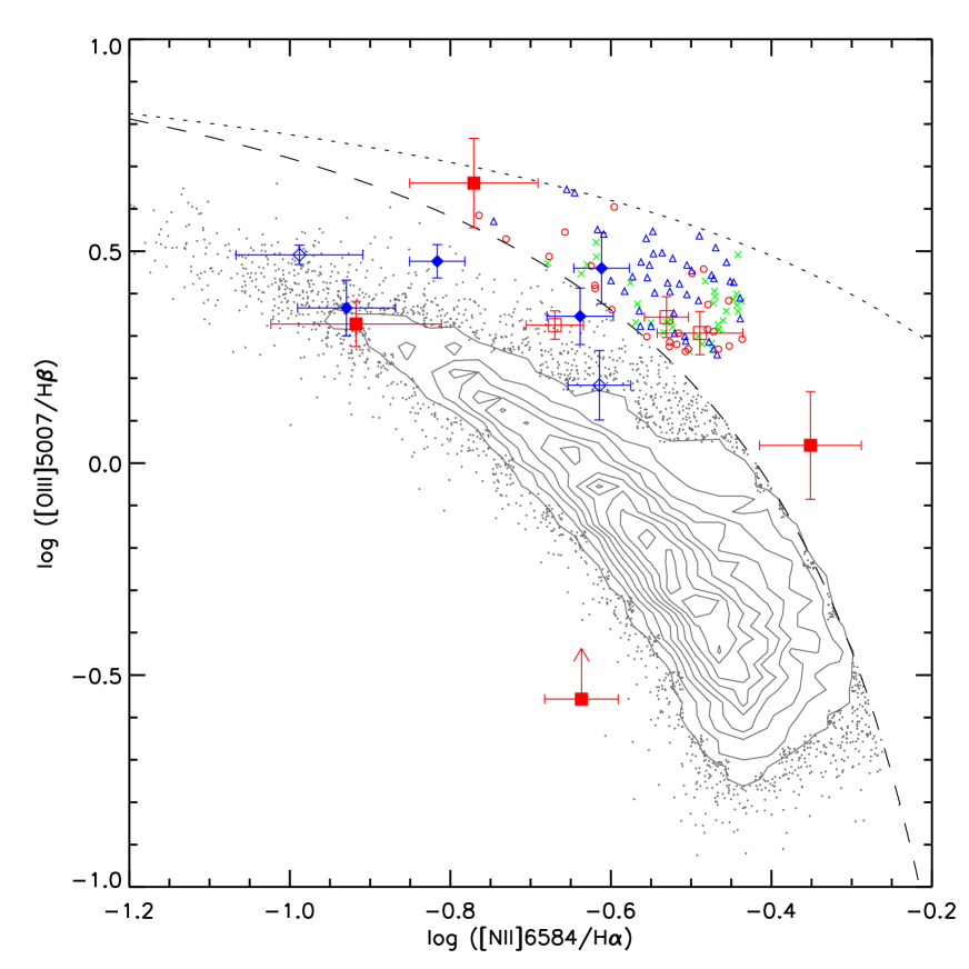
Figure 8.— H II region diagnostic diagram: log[N II]/H$\alpha$ vs. log[O III]/H$\beta$. SDSS Main, Offset-AGN, Offset-ambiguous, and Offset-SF samples are shown as grey contours with dots, blue triangles, green crosses, and red circles, respectively (see §5.2 for more information on sample selection rules). The $z\sim 1.0-1.5$ DEEP2 objects are also shown for a comparison using the same legends as in the left panel of Figure 7, and the dotted and dashed lines have the same meanings as those in Figure 7.

There is evidence that physical conditions in the H II regions of high-redshift galaxies hosting intense star formation are different from those of local H II regions (Paper I). The most common method for probing H II region physical conditions, and discriminating between star-forming galaxies and AGNs, is based on the positions of objects in the Baldwin, Phillips, & Terlevich (1981) empirical diagnostic diagrams (hereafter BPT diagrams). These plots feature the optical line ratios [N II]/H$\alpha$, [O I]/H$\alpha$, [S II]/H$\alpha$, and [O III]/H$\beta$, and have been updated by many authors, including Osterbrock & Pogge (1985), Veilleux & Osterbrock (1987), Kewley et al. (2001a, hereafter Ke01), and Kauffmann et al. (2003a, hereafter Ka03). A considerable fraction of high-redshift star-forming galaxies at both z $\sim$ 1 (paper I) and z $\geq$ 2 (Erb et al., 2006a) do not follow the local excitation sequence formed by nearby H II regions and star-forming galaxies on the emission-line diagnostic diagram of [N II]/H$\alpha$ versus [O III]/H$\beta$; on average, they lie offset upward and to the right. These differences must be taken into account when applying empirically calibrated abundance indicators to galaxy samples at different redshifts. Several possible causes for the offset have been discussed in Paper I, including differences in the ionizing spectrum, ionization parameter, electron density, and the effects of shocks and AGNs.

In Figure 7, [O III]/H$\beta$ and [N II]/H$\alpha$ ratios are plotted in the left panel for the 13 galaxies in our sample with the full set of emission lines, and the average [O III]/H$\beta$ and [N II]/H$\alpha$ ratios from the N2+O3 composite spectra are also shown in the right panel for bins at $z\sim 1.0$ and $1.4$, respectively. A subset of emission-line objects from SDSS are also shown as grey contours and dots for comparison. The dotted curve is from Ke01, representing a theoretical upper limit on the location of star-forming galaxies in the diagnostic diagram. The dashed curve is from Ka03 and serves as an empirical discriminator between star-forming galaxies and AGNs. On average, the H$\alpha$ flux of galaxies below this curve should have $<1\%$ contribution from AGNs (Brinchmann et al., 2004). The effect observed in Paper I is still present in our larger sample, in the sense that the $z\sim 1.0-1.4$ sample is, on average, significantly offset from the excitation sequence formed by star-forming galaxies from SDSS. Furthermore, the average offset for the $z\sim 1.4$ objects is larger than for those at $z\sim 1.0$. A similar, if not stronger, effect is observed in star-forming galaxies at $z\sim 2$ (Erb et al., 2006a). As discussed in Paper I, unaccounted-for stellar Balmer absorption is not the explanation for the offsets in emission-line ratios, since the corrections would shift the DEEP2 galaxies by no more than 0.1 dex downward and by an insignificant amount in [N II]/H$\alpha$.

Isolating the causes of the offset of the high-redshift samples from the local excitation sequence on the diagnostic diagram will provide important insight into the physical conditions in distant star-forming galaxies. These conditions also comprise an essential systematic factor determining the emergent strong emission-line ratios and associated calibration of chemical abundances. Unfortunately, we do not currently have a large high-redshift sample with available additional spectral features, stellar population parameters, and morphological information, which is needed for a direct study of how the diagnostic line ratios vary as functions of galaxy properties. However, as seen in Figure 7, while only a tiny fraction of the SDSS galaxies reside in the region of BPT parameter space inhabited by our most extremely offset high-redshift galaxies, in between the star-forming excitation sequence and the AGN branch, the sheer size of the SDSS sample still results in a set of $\sim 100$ such local objects. These objects can serve as possible local counterparts for our DEEP2 objects, with the added benefit of high S/N photometric, spectroscopic, and morphological information from SDSS. We will make use of this detailed information to understand the cause of the local galaxies’ offset in the BPT diagram, and, by extension, the likely cause of the offset among the high-redshift galaxies.

In the following sections, we compare in detail these anomalous SDSS objects against more typical SDSS star-forming galaxies. Accordingly, we analyze possible causes for their offset in terms of different physical conditions in the ionized regions, which include H II region electron density, hardness of the ionizing spectrum, ionization parameter, the effects of shock excitation, and contributions from an AGN. We further try to unravel possible connections between physical conditions of these anomalous SDSS objects and their host galaxy properties and use them to interpret our observations of high-redshift star-forming galaxies.

5.2. Local Counterparts: SDSS Main and Offset Samples

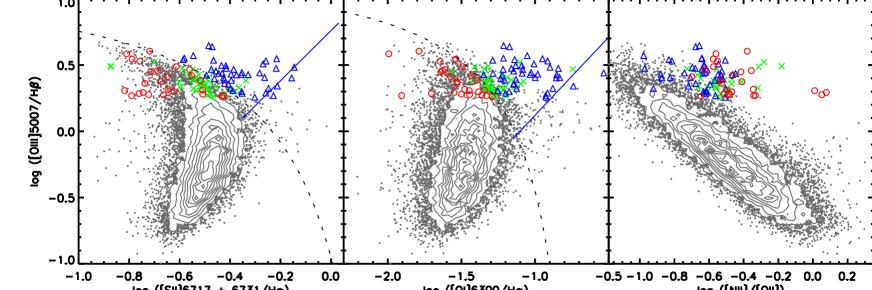
Figure 9.— H II region diagnostic diagrams. Descriptions for SDSS objects are the same as those in Figure 8. On the [O I]/H$\alpha$ and [S II]/H$\alpha$ diagrams, the dotted (blue solid) lines are empirical curves separating star-forming galaxies (Seyferts) and AGN (LINERs) from Kewley et al. (2006). The log[N II]/[O II] vs. log[O III]/H$\beta$ diagram is useful in separating ionization parameter and abundance but becomes insensitive to ionization parameter above solar metallicity (Dopita et al., 2000). The [N II]/[O II] flux ratio has been corrected for dust extinction, given the wide spacing in wavelength between [N II] and [O II].

Within this work we use the SDSS Data Release 4 (DR4; Adelman-McCarthy et al., 2006) spectroscopic galaxy sample, which contains $u$-, $g$-, $r$-, $i$-, and $z$-band photometry and spectroscopy of 567,486 objects. As described in Tremonti et al. (2004), emission-line fluxes of these galaxies were measured from the stellar-continuum subtracted spectra with the latest high spectral resolution population synthesis models by Bruzual & Charlot (2003).

Before being further divided into groups with different emission-line diagnostic ratios, our sample was selected from the 567,486 galaxy DR4 sample according to the following criteria:

(1) Redshifts in the range $0.005<z<0.25$. (2) Signal-to-noise ratio (S/N) $>$ 3 in the strong emission-lines [O II] $\lambda\lambda$3726, 3729, H$\beta$, [O III] $\lambda\lambda$4959, 5007, H$\alpha$, [N II] $\lambda$6584, and [S II] $\lambda\lambda$6717, 6731; and S/N $>$ 1 in the weak emission-line [O I] $\lambda$6300. In practice, $\sim 99$% of the objects also have [O I] $\lambda$6300 S/N$>$3. (3) The fiber aperture covers at least 20% of the total $g$-band photons. (4) Stellar population parameter estimates are available in the catalog derived using methods described by Kauffmann et al. (2003b).

The first criterion on redshift range is the same as that adopted by Tremonti et al. (2004), which enables a fair comparison with the mass-metallicity relation from their work. The second criterion selects galaxies with well-measured emission-line fluxes, required by our study based on emission-line diagnostic ratios. The S/N values were obtained using errors of the emission-line fluxes, which were first taken from the emission-line flux catalog on the MPA DR4 Web site and then scaled by the recommended factors (see the Web site for more details about the emission-line flux error). The third criterion is required to avoid significant aperture effects on the flux ratios (Kewley et al., 2005; Tremonti et al., 2004). Lower aperture fraction can cause significant discrepancies between aperture and global parameter estimates. The fourth criterion enables a comparison of stellar population properties with diagnostic emission-line ratios. Roughly 30% of the initial set of DR4 galaxies were ruled out because they do not have stellar population parameter estimates; an additional $\sim$20% was cut out according to the redshift and aperture-coverage constraints. Rules on the S/N in both strong and weak emission lines removed another $\sim$45% of the objects. In all, these selection criteria leave us with $\sim$31,000 emission-line objects, shown as grey contours and dots in Figure 7, which is about 5% of the 567,486 galaxy DR4 sample.

With the exception of one of the 13 DEEP2 objects, which lies on the part of the [N II]/H$\alpha$ versus [O III]/H$\beta$ diagram populated by many H II/AGN composites, the high-redshift galaxies on average fall between the excitation sequence of typical SDSS star-forming galaxies and the AGN branch. Although many of the DEEP2 objects have a less extreme offset relative to typical SDSS star-forming galaxies than those of the sample of Erb et al. (2006a), and the most extreme $z\sim 1.4$ objects in Paper I, there are still several that are significantly offset from the main sequence. We proceed by studying properties of the SDSS galaxies with similar [N II]/H$\alpha$ and [O III]/H$\beta$ values to those of the significantly offset DEEP2 objects, and comparing these unusual objects with typical SDSS star-forming galaxies along the excitation sequence. In this sense we further divide the SDSS sample into the “Main”, and “Offset” subgroups, as shown in Figure 8.

Objects in the Main sample are selected to lie below the Ka03 empirical curve, whereas Offset objects are located in between the Ka03 and the Ke01 curves. The Offset sample is also constrained to have log([N II]/H$\alpha$) $\leq$ -0.44 and log([O III]/H$\beta$) $\geq$ 0.26, according to the two emission-line ratios of the DEEP2 object with the second largest [N II]/H$\alpha$ value. We do not use the galaxy with the largest [N II]/H$\alpha$ value in our DEEP2 sample for the selection criteria of the two line ratios, because the number density in the composite region increases very rapidly as the AGN branch is approached, yet most of our DEEP2 galaxies clearly do not fall in that regime. Also, it is worth pointing out that, while they are significantly displaced from the local excitation sequence, more than half of the DEEP2 objects actually lie below the Ka03 curve. Indeed, the SDSS Offset sample is constructed according to our DEEP2 objects that are offset the most, in order to create a strong contrast with the Main sample. It is also representative of the $z\sim 2$ galaxies observed by Erb et al. (2006a). As we describe in §5.6, the conclusions drawn from this extreme sample are corroborated by the work of Brinchmann et al. (2008), where objects with less extreme offsets are considered and therefore should be valid for typical objects in our DEEP2 sample. Finally, the Offset sample only covers a certain range of stellar masses, so we further select the Main control sample according to the same stellar-mass range in order to ensure a fair comparison. This leaves us with $\sim$21,000 objects for the Main sample and 101 objects for the Offset sample.

Figure 9 displays how objects in the Offset sample are distributed in the additional BPT diagrams featuring [O I]/H$\alpha$ and [S II]/H$\alpha$. These plots indicate that Offset objects selected solely on the basis of their [O III]/H$\beta$ and [N II]/H$\alpha$ ratios span a diverse range of properties in other physical parameter spaces. High [O I]/H$\alpha$ and [S II]/H$\alpha$ both occur when there is a hard ionizing radiation field, including significant contribution from X-ray photons. In this case, there is an extended, partially ionized zone, where H I and H II coexist, and [O I] and [S II] are dominant forms of O and S. The extended zone of partially ionized H does not exist in H II regions photoionized by OB stars (Evans & Dopita, 1985; Veilleux & Osterbrock, 1987). High [O I]/H$\alpha$ and [S II]/H$\alpha$ are also produced in gas that has been heated by fast, radiative shocks, which also produce partially ionized shock-precursor regions (Dopita & Sutherland, 1995, 1996). Material in supernova remnants provides an example of shocked gas. While it is sensitive to shocks, [S II] is more susceptible to collisional de-excitation than [O I], given its critical density (2$\times 10^{3}$ cm^-3), as opposed to that of [O I] (2$\times 10^{6}$ cm^-3), and therefore might be suppressed in regions of high electron densities (Dopita, 1997; Kewley et al., 2001b). Another point worth mentioning is that [O I]/H$\alpha$ should reveal larger differences in regions ionized by hard spectrum as opposed to that of stars, than [S II]/H$\alpha$ does. This is because the ionization potential of [O I] matches that of H I, so [O I] enhancement should reflect increased presence of partially ionized zone. However, [S II] exists in both completely and partially ionized zones. So the contrast between AGN- and stellar-ionized regions for [S II]/H$\alpha$ is not as great as that for [O I]/H$\alpha$.

In summary, the various locations of the Offset objects on the [O I]/H$\alpha$ and [S II]/H$\alpha$ diagrams indicate different levels of contribution from AGN and shock excitations to the emerging spectra. We therefore further divide the Offset sample on the [O I]/H$\alpha$ and [S II]/H$\alpha$ diagrams, according to the theoretical scheme for classifying starburst galaxies and AGNs (Kewley et al., 2001a, 2006). It is worth noting here that all objects in the Offset sample have S/N$>$3 in both [S II] and [O I] emission lines, so this division should not be compromised by spurious measurements. While there may still be a low-level ($<10$%) AGN contribution to the spectra of objects classified as starbursts by this scheme, it serves as a rough guide to the range of properties in the Offset sample. This classification leaves us with (1) “Offset-AGN” (43), where objects lie above both the Ke01 curves of the two diagrams; (2) “Offset-ambiguous” (33), where objects lie above one Ke01 curve and under the other one; and (3) “Offset-SF” (25), where objects lie below both the Ke01 curves. The division of Offset-AGN and Offset-SF is only based on hardness of the ionizing spectrum and the contribution of shock excitation. We show in Section 5.4 that these two offset samples have different host galaxy properties.

5.3. H II Region Emission-Line Diagnostic Ratio, Physical Conditions, and Galaxy Properties

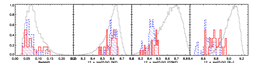
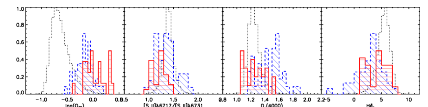
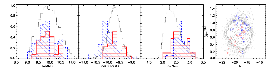
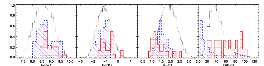
Figure 10.— Distribution of row (1): redshift and metallicities based on various strong-line indicators; row (2): ionization-parameter indicator log($O_{32}$), electron density indicator [S II] $\lambda 6717$/[S II] $\lambda 6731$, D${}_{n}(4000)$ and H$\delta_{A}$; row (3): stellar mass, fiber-corrected specific star formation rate, $r$-band Petrosian concentration index $C=R_{90}/R_{50}$, and color-magnitude diagram; row (4): surface mass density log($\mu_{\star}$), SFR surface density log($\dot{\Sigma}_{\star}$), $R_{50}(z)$, which is the radius enclosing 50% of the Petrosian $z$-band luminosity of a galaxy, and H$\alpha$ emission equivalent widths, for the SDSS Main (black dotted line), Offset-AGN (blue dashed line), and Offset-SF samples (red solid line; see §5.2 for more information). For clarity, the distribution functions are normalized to three different levels, with the maxima being 1.0, 0.7, and 0.5 for the SDSS Main, Offset-AGN, and Offset-SF samples, respectively.

In order to determine the origin of the observed difference in emission-line ratios between the Main and Offset samples, we consider a large set of galaxy properties. Measurements of emission lines as well as photometric, physical, and environmental properties of stellar population are available for our SDSS samples. In this section, we describe the galaxy properties of interest, while in the following section, a comparison of the Main and Offset sample distributions in these properties is presented.

First, using emission-line ratios, we examine the main factors controlling the emission-line spectrum in an H II region, i.e., the gas phase metallicity, the shape or hardness of the ionizing radiation spectrum, and the geometrical distribution of gas with respect to the ionizing sources, which can be represented by the mean ionization parameter and electron density (Dopita et al., 2000). Several H II region emission-line ratios can be used as diagnostics of these factors.

Apart from the N2 and O3N2 indicators, we also use the ratio N2O2 $\equiv$ log([N II] $\lambda$6584/[O II] $\lambda\lambda$3726, 3729), suggested by van Zee et al. (1998), as an abundance diagnostic for SDSS objects, because N2O2 is virtually independent of ionization parameter and also strongly sensitive to metallicity. This indicator is monotonic between 0.1 and over 3.0 times solar metallicity (Dopita et al., 2000; Kewley & Dopita, 2002). Concerns about reddening correction and reliable calibration over such a large wavelength baseline have hampered the use of this ratio. As shown in Kewley & Dopita (2002), however, the use of classical reddening curves and standard calibration are quite sufficient to allow this [N II]/[O II] diagnostic to be used as a reliable abundance indicator. The Bresolin (2007) calibration of N2O2 is used to infer oxygen abundance. We also use the $R_{23}\equiv$ log{([O II] $\lambda$3727 + [O III] $\lambda\lambda$4959, 5007)/H$\beta$} parameter, introduced by Pagel et al. (1979), as an abundance indicator, to make comparison with several works (Lilly et al., 2003; Savaglio et al., 2005), although this indicator has some well-documented drawbacks (e.g. Kobulnicky et al., 1999; Kewley & Dopita, 2002).

$O_{32}\equiv$ log([O III] $\lambda$5007/[O II] $\lambda\lambda$3726, 3729) is used as an indicator of the ionization parameter (McGaugh, 1991; Dopita et al., 2000). However, $O_{32}$ is sensitive to both ionization parameter and abundance; both low ionization parameter and high abundances produce low values of $O_{32}$ (Dopita et al., 2000; Kewley & Dopita, 2002). Thus, when $O_{32}$ is used as a diagnostic of the relative ionization parameters of different samples, the metallicities of these samples must also be taken into account for a fair comparison. A diagnostic plot, for example, N2O2 versus $O_{32}$, can be used to separate ionization parameter and abundance. The ratio [S III]/[S II] provides another diagnostic of the ionization parameter, which is independent of metallicity except at very high values of the ratio (Kewley & Dopita, 2002). Unfortunately, the SDSS spectra do not cover [S III] $\lambda\lambda$9069, 9532 from SDSS, so it is not included here.

Finally, [S II] $\lambda 6717$/[S II] $\lambda 6731$ is adopted as an electron-density indicator. We do not use the density-sensitive ratio, [O II] $\lambda 3726$/[O II] $\lambda 3729$, since this doublet is typically blended in SDSS spectra.

We note that emission-line ratios, such as $O_{32}$, N2O2, and $R_{23}$ have large separations in wavelength and thus need to be corrected for dust reddening. The Balmer decrement method with the reddening curve of Calzetti et al. (2000) is used to correct these quantities for dust extinction, assuming an intrinsic ratio of $H\alpha/H\beta=2.78$, appropriate for $T_{e}=10,000$ K.

Next, we turn to the question of the stellar populations and structural and environmental properties of the Main and the Offset sample host galaxies. To examine stellar ages, we adopt the narrow definition of the 4000 ${\rm\AA}$ break denoted as D${}_{n}(4000)$ (Balogh et al., 1999), which is small for young stellar populations and large for old, metal-rich galaxies (Kauffmann et al., 2003b). We use the H$\delta_{A}$ index as an indicator of recent starburst activities (e.g. Kauffmann et al., 2003b; Worthey & Ottaviani, 1997). Strong H$\delta$ absorption lines arise in galaxies that experienced a burst of star formation that ended $\sim$0.1-1 Gyr ago. For galaxy morphology, we use the standard concentration parameter defined as the ratio $C=R_{90}(r)/R_{50}(r)$, where $R_{90}(r)$ and $R_{50}(r)$ are the radii enclosing 90% and 50% of the Petrosian $r$-band luminosity of the galaxy. For galaxy size, we study $R_{50}(z)$, the radius enclosing 50% of the Petrosian $z$-band luminosity of a galaxy. We also examine the surface mass density $\mu_{\star}$, defined as $M_{\star}/[2\pi R^{2}_{50}(z)]$ (Kauffmann et al., 2003c), the SFR surface density $\dot{\Sigma}_{\star}\equiv{\rm SFR}/[2\pi R^{2}_{50}(r)]$, where we use a radius defined in the $r$ band rather than the $z$ band, as it is more appropriate for H$\alpha$ luminosities. Additional parameters include the fiber-corrected specific star formation rate SFR/M_⋆, H$\alpha$ equivalent width (EW), and the color-magnitude diagram $(g-i)^{0.1}$ versus $M_{r}$, where $(g-i)^{0.1}$ denotes the $(g-i)$ color $k$-corrected to $z=0.1$, and $M_{r}$ stands for the $k$-corrected $r$-band absolute magnitude (Kauffmann et al., 2003b). In order to search for any environmental dependence of the Offset sample properties, we count the number of spectroscopically observed galaxies that are located within 2 Mpc in projected radius and $\pm$500 km s^-1 in velocity difference from each object in our SDSS samples. Here we follow the procedures described in Kauffmann et al. (2004), constructing a volume-limited tracer sample using the SDSS DR4 data.

5.4. Comparison with Typical SDSS Star-forming Galaxies

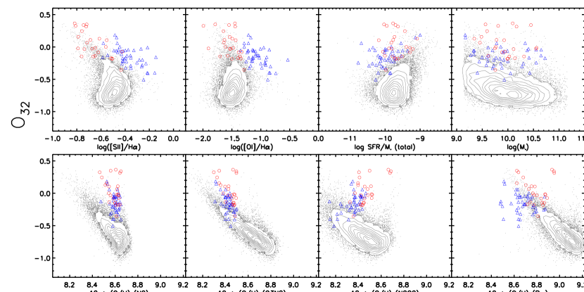
Figure 11.— Ionization-parameter indicator $O_{32}$, as a function of various parameters. Descriptions are the same as those in Figure 9.

In this section, we compare the properties of Offset and Main sample objects, in terms of their H II region physical conditions, stellar populations, structural parameters, and environments. In particular, we find striking differences in H II region ionization parameter, electron density, galaxy size, and star formation rate surface density. Figure 10 shows relative distributions of diagnostic-line ratios and galaxy properties of the SDSS Main, Offset-AGN, and Offset-SF samples. For clarity, the distribution functions are normalized to three different levels, with the maxima being 1.0, 0.7 and 0.5 for the SDSS Main, Offset-AGN, and Offset-SF samples, respectively.

First, we consider H II region physical conditions. Compared to the Main sample, both Offset samples on average have larger ionization parameters. The Offset-SF and Offset-AGN samples have $O_{32}=0.0$ and -0.2, respectively, as opposed to -0.7 for the Main sample. Here and throughout, we refer to the median values of the distributions. Since $O_{32}$ also depends on metallicity, we need to make a fair comparison for the ionization parameter at a fixed metallicity. Figure 11 shows $O_{32}$ as a function of several emission-line diagnostic ratios and galaxy properties. In the lower four panels, we can see that, regardless of which metallicity indicator is used, the Offset-SF sample has bigger $O_{32}$ values than the Main sample at a fixed strong-line indicator value. Therefore, the Offset-SF sample has larger average ionization parameter than Main sample objects having similar metallicities, independent of the metallicity indicator. Compared with the Main sample, all indicators except $R_{23}$ suggest that the Offset-AGN has higher ionization parameters at fixed metallicities.

The Offset-SF sample also has significantly larger electron densities, on average, than the Main sample ([S II] $\lambda 6717$/[S II] $\lambda 6731$ of $\sim$1.23 compared to $\sim$1.40, corresponding to electron densities of $\sim$208 cm^-3 compared to $\sim$47 cm^-3), whereas the Offset-AGN sample has only slightly higher electron densities than those of the Main sample ([S II] $\lambda 6717$/[S II] $\lambda 6731$ of $\sim$1.37, corresponding to electron densities of $\sim$67 cm^-3). As discussed in Paper I, for fixed ionization parameter, metallicity, and input ionizing spectrum, the photoionization models presented in Kewley et al. (2001a) display a dependence on electron density, in the sense that model grids with higher electron density have an upper envelope in the space of [O III]/H$\beta$ versus [N II]/H$\alpha$ that is offset upward and to the right, relative to model grids with lower electron density. This theoretical shift in the BPT diagram due to increased electron density is qualitatively reflected in the properties of Offset-SF objects.

Next, we consider photometric and spectroscopic stellar population properties. The Offset-SF sample is similar to the Main sample in terms of median color [$(g-i)^{0.1}$ $\sim$ 0.64 compared to $\sim$0.66], stellar age [the same value of D_n(4000) = 1.24], and fiber-corrected specific star formation rates (the same value of $\log((SFR/M_{\star})\mbox{ yr}^{-1})=-9.7$), whereas the Offset-AGN sample has redder colors [$(g-i)^{0.1}$ of $\sim$0.86], older stellar ages [D_n(4000) = 1.50], and lower specific star formation rates ($\log((SFR/M_{\star})\mbox{ yr}^{-1})=-10.0$). Also, the Offset-SF sample has a larger H$\alpha$ EW than the Main sample (62 ${\rm\AA}$ compared to 40 ${\rm\AA}$), whereas the Offset-AGN sample has a much smaller H$\alpha$ EW (15${\rm\AA}$). The Offset-SF sample has a smaller burst fraction in stellar mass than the Main sample (H$\delta_{A}$ of 4.3 compared to 5.5), while the discrepancy between the Offset-AGN and Main samples is even larger (H$\delta_{A}$ of 3.3 compared to 5.5).

In terms of galaxy structure, the Offset-SF sample has larger concentration ($C$ = 2.58 compared to 2.36), smaller half-light radii [$R_{50}(z)$ of 1.2 kpc compared to 1.9 kpc], higher surface stellar mass density [log($\mu_{\star}$) of 8.78 M_⊙ kpc^-2 compared to 8.61 M_⊙ kpc^-2], and higher SFR surface density [log($\dot{\Sigma}_{\star}$) of -0.86 M_⊙ yr^-1 kpc^-2 compared to -1.12 M_⊙ yr^-1 kpc^-2] than the Main sample, whereas the Offset-AGN has larger concentration ($C$ of 2.66), moderately smaller sizes [$R_{50}(z)$ of 1.5 kpc], moderately higher surface stellar mass density [log($\mu_{\star}$) of 8.68 M_⊙ kpc^-2], and similar SFR surface density [log($\dot{\Sigma}_{\star}$) of -1.12 M_⊙ yr^-1 kpc^-2].

In terms of environment, we find that 90%-95% of objects in the Main, Offset-SF, and Offset-AGN samples have zero or one neighbor, the lowest density bin in Kauffmann et al. (2004). Furthermore, the distributions of environments for the Offset samples are similar to that of the Main sample. Therefore, it appears that the vast majority of galaxies considered here reside in the lowest density environment defined by Kauffmann et al. (2004). This result is not surprising, as our SDSS samples all contain emission-line galaxies, which are more likely to be found in low-density environments (Kauffmann et al., 2004). Currently we have too few Offset objects to draw any solid conclusion about the question on galaxy environmental dependence.

Groves et al. (2006) suggest that the offset on the BPT diagram seen in some high-redshift galaxies is mostly caused by contribution from AGNs, as they found properties of their candidate low-metallicity H II/AGN composites similar to those of the host galaxies of AGNs (Kauffmann et al., 2003a; Heckman et al., 2004); these objects have on average significantly higher stellar masses, older stellar populations, and redder colors than the sample of pure star-forming galaxies used for comparison. Groves et al. (2006) arrive at this conclusion after constructing their offset sample in a region bounded by the Ka03 and the Ke01 curves in the [N II]/H$\alpha$ versus [O III]/H$\beta$ diagram, and the Seyfert branch [log([O III]/H$\beta$) $\geq$ 3log([N II]/H$\alpha$)]. When we reproduced their offset sample, we found the median values of log([N II]/H$\alpha$) $\sim$ -0.286 and log([O III]/H$\beta$) $\sim$ -0.024, whereas the corresponding values for our DEEP2 objects are -0.638 and 0.344. As the density of objects increases rapidly towards increasing [N II]/H$\alpha$, the offset sample definition of Groves et al. (2006) is weighted heavily towards H II/AGN composites and not necessarily representative of the average [N II]/H$\alpha$ or [O III]/H$\beta$ of high-redshift galaxies. Furthermore, it is not clear that their “typical” comparison sample, which was defined as all galaxies within $\pm$0.05 dex of [-0.55, 0.10] in the [N II]/H$\alpha$ versus [O III]/H$\beta$ diagram, represents a fair one, as they have not controlled for any galaxy property. Given the strong correlations among galaxy properties, it is crucial to compare galaxies that are similar in at least some basic parameters. Here we want to emphasize that in order to make a controlled comparison, the Main sample was selected to have similar range and median of stellar masses as that of the Offset sample. The Main sample also has a similar median [N II]/H$\alpha$ value. With this controlled comparison of typical and Offset SDSS objects, we find that the unusual objects on the BPT diagram are populated not only by likely AGN hosts (Offset-AGN) but also by the Offset-SF sample, most of which do not resemble typical AGN-host galaxies. Furthermore, there is no segregation of the two offset samples in the [N II]/H$\alpha$ versus [O III]/H$\beta$ diagram.

As suggested in Groves et al. (2006), another possible test of the presence of an AGN would require the detection of either He II $\lambda$4686 or [Ne V] $\lambda$3426 lines. The [Ne V] $\lambda$3426 line is not redshifted into the SDSS band for the majority of our objects: we have only four such objects in Offset-AGN, of which the spectra near [Ne V] $\lambda$3426 are too noisy to provide any meaningful constraints. The He II $\lambda$4686 line is expected to be very weak: a 20% AGN contribution to H$\beta$ implies He II/H$\beta$ = 0.05. Note that besides the AGN photoionization, possible mechanisms for producing He II emission also include hot stellar ionizing continua and shock excitation (Garnett et al., 1991). Another important goal is to infer metallicities of the Offset-SF objects using a method that is independent of strong-line indicators, since these objects have abnormal strong-line ratios. A more calibration-independent way to address metallicity is through the classic $T_{e}$ method, which relies on measuring weak auroral lines. Both the test of the presence of AGNs, and the determination of metallicity with the direct $T_{e}$ method, require the measurement of very weak lines. These measurements become feasible through the use of composite spectra.

5.5. SDSS Composite Spectra

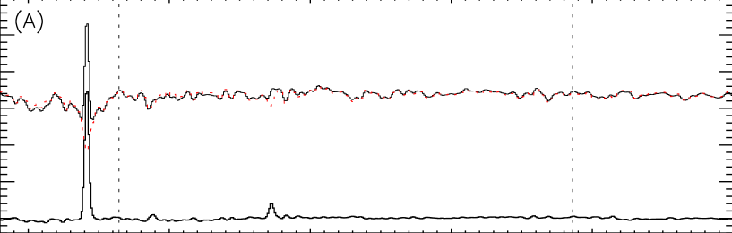
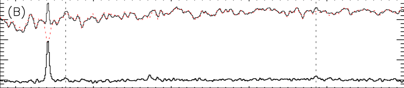
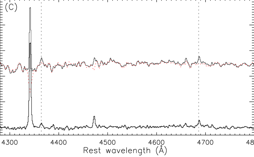
Figure 12.— SDSS composite spectra. For clarity, only the portion of the spectrum containing the weak emission lines of interest is presented here. The original composite and stellar-continuum-subtracted spectra for samples (A) Main, (B) Offset-AGN, and (C) Offset-SF are shown as black solid curves. Stellar-continuum fits using Bruzual & Charlot (2003) population synthesis models are plotted as red dotted curves. The [O III] $\lambda$4363 and He II $\lambda$4686 lines are marked by dotted lines.

In order to measure He II $\lambda$4686 as another test of possible AGN contribution to the ionizing spectrum, and [O III] $\lambda$4363 to infer the oxygen abundance using the $T_{e}$ method, we construct composite spectra for both Offset-SF and Offset-AGN objects. For comparison, we also make composite spectra for the Main sample. We adopt the same method of making composite spectra used for our DEEP2 objects, employing median scaling to preserve the relative fluxes of the emission features. The variance spectrum is combined in the same way and the error for the corresponding composite spectrum is the square root of the composite variance spectrum divided by the number of objects.

The stellar continuum was modelled over the rest-frame wavelength range of 3800 - 7500 ${\rm\AA}$ and then subtracted from the composite spectra, with a method similar to the one described in Tremonti et al. (2004) and Brinchmann et al. (2004). This technique (Charlot & Bruzual, 2007, private communication) relies on the Bruzual & Charlot (2003) stellar population synthesis model, but with two major improvements. First, the number of the metallicity grids was expanded from three to four; second, and most importantly, the stellar continuum fitting was carried out using both the STELIB (Le Borgne et al., 2003) and the MILES (Sánchez-Blázquez et al., 2006) libraries of observed stellar spectra. Models using the MILES library fit the data better than those with the STELIB one, in terms of the agreement around Balmer lines. It is especially essential to obtain a reasonable stellar continuum fit near H$\gamma$, which is very close in wavelength to the weak [O III] $\lambda$4363 auroral line. Models using the STELIB library tend to over-estimate stellar continua, especially around Balmer lines. We therefore adopt the stellar continuum models based on the MILES library.

The resultant continuum-subtracted spectra, along with the original composite spectra and the best-fit model of the stellar continua, are shown in Figure (12). We only present portions of the entire composite spectra to enable scrutiny of the relevant weak lines ([O III] $\lambda$4363 and He II $\lambda$4686) and our capability of making a reasonably good stellar continuum fit. The corresponding error spectra are estimated by combining the measurement error for the composite spectra and the systematic uncertainties from the stellar continuum fitting. The systematic error from the stellar continuum fitting is estimated using the rms of a portion of the continuum-subtracted spectrum, which is relatively free of emission-line features. This method of estimating continuum fit error is motivated by the fact that the rms would be zero if the fitting was ideally good and if there were no emission-line features. At all of the wavelengths considered, the systematic error is significantly larger than the measurement error for the composite spectra and therefore dominates the total error budget. Emission-line fluxes and flux ratios with the total uncertainties are given in Table 5.

There are a few caveats that must be mentioned in the analysis of composite spectra described here. First, we are averaging over tens of thousands of galaxies for the SDSS Main sample and dozens of galaxies for the Offset-SF and Offset-AGN samples; second, for each single galaxy, we are dealing with integrated spectra containing contributions from multiple H II regions, which may show a range of metallicities, ionization parameters, ionizing spectra, and electron densities. Also, even though we select the samples to have fiber apertures covering more than 20% of the total $g$-band photons, because of the presence of radial gradients in galaxy properties, uncertainties still remain since the spectrum is weighted towards the nucleus. Despite these caveats, however, we want to emphasize that the analysis of composite integrated fibre-based spectra is still meaningful in terms of determining average properties and the relative differences among samples.

Table 5Emission-line flux measurements of SDSS composite spectra.

Sample	F[OII]λλ3726,3729	F[OIII]λ4363	FHeIIλ4686	FHβ	F[OIII]λ4959	F[OIII]λ5007	F[OI]λ6300
Main	327.3$\pm$0.3	0.6$\pm$0.2	1.4$\pm$0.2	153.5$\pm$0.2	45.2$\pm$0.1	137.0$\pm$0.3	19.1$\pm$0.2
Offset-AGN	271.9$\pm$0.8	2.8$\pm$0.5	4.9$\pm$0.5	90.4$\pm$0.5	86.4$\pm$0.2	261.7$\pm$0.6	24.3$\pm$0.6
Offset-SF	629.1$\pm$1.0	7.1$\pm$0.6	12.5$\pm$0.7	321.0$\pm$0.7	266.6$\pm$0.3	807.4$\pm$0.8	38.8$\pm$0.7
Sample	FHα	F[SII]λ6717	F[SII]λ6731	$\frac{{\rm F_{[OIII]\lambda\lambda 4959,5007}}}{{\rm F_{[OIII]\lambda 4363}}}$	$\frac{{\rm F_{HeII\lambda 4686}}}{{\rm F_{H\beta}}}$	$\frac{{\rm F_{[OI]\lambda 6300}}}{{\rm F_{H\alpha}}}$	$\frac{{\rm F_{[SII]\lambda\lambda 6717+6731}}}{{\rm F_{H\alpha}}}$
Main	633.6$\pm$0.3	117.6$\pm$0.3	83.9$\pm$0.3	249$\pm$82	0.009$\pm$0.001	0.0301$\pm$0.0004	0.3180$\pm$0.0006
Offset-AGN	337.3$\pm$0.7	80.6$\pm$0.6	58.5$\pm$0.6	110$\pm$19	0.054$\pm$0.006	0.0720$\pm$0.0018	0.4124$\pm$0.0028
Offset-SF	1272.8$\pm$0.9	170.6$\pm$0.8	137.3$\pm$0.8	129$\pm$11	0.039$\pm$0.002	0.0305$\pm$0.0006	0.2419$\pm$0.0009

5.5.1 AGN Contribution

The composite spectra we construct can be used to address the level at which AGN ionization contributes to the anomalous emission-line ratios, discovered in both nearby SDSS Offset objects and high-redshift DEEP2 galaxies. Based on their [S II]/H$\alpha$ and [O I]/H$\alpha$ ratios, we expect the Offset-AGN objects to have a non-negligible contribution to their ionization from AGNs and/or shock heating. Based on the composite spectrum, we can also probe the weaker He II line, which is another indicator of AGN activity.

From the He II/H$\beta$ ratio (0.054$\pm$0.006), we can see that the Offset-AGN sample may have up to $\sim$20% AGN contribution to the Balmer emission lines (Groves et al., 2006). The Offset-SF sample, on the other hand, shows a lower level of possible AGN contamination (He II/H$\beta$ of 0.039$\pm$0.002). This distinction is also suggested by the different host-galaxy properties of the two samples. The Offset-AGN objects with similar stellar masses to the Main sample have redder colors, older stellar populations, lower starburst stellar mass fraction, smaller H$\alpha$ EWs, and smaller specific star formation rates, which are similar to host galaxies of AGN (Kauffmann et al., 2003a), whereas the Offset-SF sample is similar to the Main sample in terms of these galaxy properties. Furthermore, by construction, the Offset-SF objects have low [S II]/H$\alpha$ and [O I]/H$\alpha$ in the range favored for typical star-forming galaxies.

We note, however, that the Offset-SF sample still has a higher value of He II/H$\beta$ than the Main sample (0.009$\pm$0.001). There might be some mixing with the Offset-AGN objects because of uncertainties in emission-line diagnostic ratios. Indeed, three objects in the Offset-SF sample have cross-identifications with $ROSAT$ sources, and two of them have optical spectra indicating broad Balmer lines. However, $\sim$90% of the Offset-SF sample show no evidence of AGNs in terms of $ROSAT$-source cross-identifications and broad Balmer lines. In addition, we have examined the He II/H$\beta$ ratios from individual galaxy spectra in the Offset-SF sample, finding that five objects (including the three with $ROSAT$ cross-identifications) of the 25 have He II/H$\beta$ $\sim$ 0.05-0.10, while the remaining 20 objects all have He II/H$\beta$ $\lesssim$ 0.01, similar to the typical He II/H$\beta$ of the Main sample. Even the five objects with He II/H$\beta$ $\sim$ 0.05-0.10 could have other possible ionizing sources including hot stars and shocks (Garnett et al., 1991). It is worth mentioning that nondetection in $ROSAT$ or broad Balmer lines cannot fully exclude the possibility of AGN contamination, as the majority of obscured AGNs are completely absorbed in the soft X-ray range and do not show broad Balmer lines. However, if the dominant cause of the Offset-SF on the BPT diagram for our Offset-SF sample was mildly obscured AGN contamination, namely, if their optical spectra were contaminated by AGN ionization at a lower level than the Offset-AGN sample, then we would expect them to exhibit intermediate emission-line diagnostic ratios and host-galaxy properties, relative to the Main and the Offset-AGN samples. This is not the case. Instead, the Offset-SF objects have even higher ionization parameters and electron densities than the Offset-AGN sample, relative to the Main sample. In addition, as discussed in §5.4, Offset-SF objects have host-galaxy properties different from those of typical weak AGNs in SDSS (Kauffmann et al., 2003a). Therefore, it appears that AGN excitation does not provide the dominant cause of the anomalous emission-line ratios for most of the Offset-SF sample.

5.5.2 Electron Temperature and Oxygen Abundance

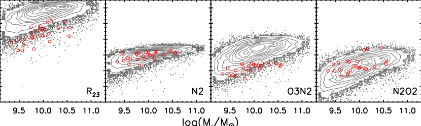
Figure 13.— Mass-metallicity relation for the SDSS Main (grey contours) and Offset-SF (red open circles) samples, based on various strong-line indicators. Calibrations are from Zaritsky et al. (1994, for $R_{23}$), Pettini & Pagel (2004, for N2 and O3N2), and Bresolin (2007, for N2O2), respectively.

Table 6Physical Quantities from SDSS composite spectra.

Sample	Ne	Te[O III]	Te[O II]	O+/H+	O++/H+	12 + log(O/H)
Main	28$\pm$ 5	0.950${}^{+0.124}_{-0.072}$	0.965${}^{+0.087}_{-0.050}$	13.2${}^{+3.7}_{-4.1}$	3.7$\pm$1.3	8.23${}^{+0.11}_{-0.17}$
Offset-SF	190$\pm$12	1.170${}^{+0.039}_{-0.033}$	1.119${}^{+0.027}_{-0.023}$	6.5$\pm$0.6	5.2$\pm$0.5	8.07$\pm$0.04

By making composite spectra, and hence enhancing the S/N of weak auroral lines, we can determine metallicities with a method independent of strong-line indicators. We have already discussed the fact that the Offset-SF objects have larger ionization parameters, as indicated by their higher $O_{32}$ values. However, it is still unclear whether the Offset-SF sample has comparable metallicity with the Main one, on average, as suggested by N2 and N2O2, or if it has $\sim$0.3 dex lower metallicity, as suggested by O3N2 and $R_{23}$. Settling this question is important for multiple reasons.

First, gas-phase metallicity and electron temperature, themselves, serve as key parameters of H II regions. Second, understanding the relative metallicities of the Main and the Offset-SF samples on average can help us determine the difference in average ionization parameter quantitatively. If the Offset-SF sample has comparable metallicities with the Main sample, their ionization-parameter difference would be very large; on the other hand, if the Offset-SF sample has much lower metallicities than the Main one does, their ionization-parameter difference would be much smaller, since both lower metallicity and higher ionization parameter can cause large $O_{32}$. Finally, if the Offset-SF objects actually have much lower metallicities than the Main objects, then they will not follow the local mass-metallicity relation (Tremonti et al., 2004), given their comparable stellar masses.

In order to determine oxygen abundances using the direct method, estimates of both the electron density and temperature are required. Based on the ratio [S II] $\lambda$6717/[S II] $\lambda$6731, we establish that on average all of our objects are in the low-density regime. Then using the five-level atom program nebular implemented in IRAF/STSDAS (Shaw & Dufour, 1995), we derive the electron temperature $T$[O III] from the ratio of auroral line [O III] $\lambda$4363 to nebular lines [O III] $\lambda\lambda$4959, 5007 (Osterbrock, 1989) and correct for dust extinction using the Balmer decrement method. As for $T$[O II], we adopt a simple scaling relation between the temperatures in different ionization zones of an H II region predicted by the photoionization models of Garnett (1992):

$$T{\rm[O\,\,II]}=0.70T{\rm[O\,\,III]}+3000\,\,{\rm K},$$ (3)

which is applicable in a wide range of $T$[O III] (2000-18,000 K). Ionic abundances O⁺⁺/H⁺ and O⁺/H⁺ are then determined using programs in the nebular package, and, finally, we obtain the total gas phase oxygen abundance assuming O/H = (O⁺ + O⁺⁺)/H⁺. The results are summarized in Table 6.

First, the Offset-SF sample has $\sim$2200 K higher electron temperatures than the Main one does on average. These objects are unusual in the sense that they have higher electron densities and electron temperatures, hence ambient interstellar pressures assuming pressure equilibrium between H II regions and ambient gas, and larger ionization parameters. It is not clear what is at the root of the special H II region physical conditions, in terms of galaxy properties, or larger scale environments. However, in the simple theoretical estimates for local starburst galaxies, the ISM pressure scales roughly linearly with the SFR surface density (e.g., Thompson et al., 2005). Indeed, the Offset-SF sample has several prominently related properties, including higher concentration ($r$-band Petrosian concentration index $R_{90}/R_{50}$ of $\sim$2.6 compared to $\sim$2.4), smaller half-light radii [$R_{50}(z)$ of 1.2 kpc compared to 1.9 kpc], and most notably, higher SFR surface density [log($\dot{\Sigma}_{\star}$) of -0.86 M_⊙ yr^-1 kpc^-2 compared to -1.12 M_⊙ yr^-1 kpc^-2)], as shown in Figure 10, compared to typical star-forming galaxies. This higher SFR surface density may therefore account for the higher interstellar pressure seen in the H II regions of Offset-SF objects.

It is also possible to relate electron temperature, electron density, and ionization parameter in a single H II region, through the classical picture of Strömgren (1939). With higher ambient interstellar pressure due to higher electron densities and temperatures, H II regions are surrounded by denser molecular gas dust and therefore have smaller radii under the stall condition. In an idealized case of a fully ionized spherical H II region with pure hydrogen, the radius $R$ of the ionized region is given by $R=[3Q/(4\pi N_{e}^{2}\alpha_{B})]^{1/3}$, where $Q$ is the rate of emission of hydrogen ionizing photons, and $\alpha_{B}$ is the case B recombination coefficient (Osterbrock, 1989). The ionization parameter $U$ defined by $[F/4\pi cR^{2}N_{{\rm HII}}]$, where $F$ is the flux of ionizing photons, $c$ is the speed of light, and $N_{{\rm HII}}$ is the particle density in H II region, is then proportional to $N_{e}^{1/3}$ for a given central hot star. Therefore, in this simple picture, H II regions with higher electron densities and temperatures will have higher ionization parameters. Accordingly, the higher electron densities and temperatures inferred from the integrated spectra of the Offset-SF objects may result in the observed higher ionization parameters as well.

Second, the Offset-SF sample has $\sim$0.16 dex lower metallicities than the Main sample. Note that the absolute abundance values inferred using the $T_{e}$ method are significantly lower than those based on any strong-line indicators. This difference may stem from temperature fluctuations in H II regions and the strong $T_{e}$ dependence of line emissivities, from which the net effect is that the electron temperature derived from auroral lines tends to overestimate the real temperature and hence systematically underestimate the abundance (Garnett, 1992). Therefore, we only focus on relative differences based on the same method between the Offset-SF and Main samples. Given that the Offset-SF and Main samples are characterized by similar average stellar masses, this difference in average metallicity suggests that Offset-SF objects do not follow the local mass-metallicity relation, in addition to being more compact and sustaining higher interstellar pressures than the Main sample.

To investigate this question further, we examine several versions of the mass-metallicity relation for the Offset-SF and the Main objects, based on different strong-line metallicity indicators. Figure 13 includes these mass-metallicity correlations for both the Main and the Offset-SF samples, demonstrating that one would draw different conclusions about the relationship between the Offset-SF and the Main samples, depending on which strong-line indicator was used. Between the Main and Offset-SF samples, the relative average metallicity differences at fixed mass based on $R_{23}$, N2, O3N2, and N2O2 are $\sim$0.28, 0.00, 0.18, and 0.00 dex, respectively. This ambiguity could be understood as the result of adopting the same calibration for samples with different physical conditions, of which the most important are ionization parameter and electron density.

The discrepancy between conclusions drawn from the strong-line indicators and the $T_{e}$ method can be understood using the photoionization models of Kewley & Dopita (2002). For example, according to $R_{23}$, the average metallicity difference between the Offset-SF and Main samples is $\sim$0.28 dex, whereas this metallicity difference based on the $T_{e}$ method is $\sim$0.16 dex. This $\sim$0.12 dex discrepancy can be explained by examining the theoretical grids in the $R_{23}$ versus 12 + log(O/H) space, given by photoionization models with different values of electron density and ionization parameter. If the incorrect assumption is adopted that both the Main and Offset-SF samples have electron densities $N_{e}\sim 10$ cm^-3 and ionization parameters $q=3\times 10^{7}\mbox{cm s}^{-1}$ – values appropriate for the Main but not Offset-SF sample – we obtain that the Offset-SF sample is $\sim 0.25$ dex lower in oxygen abundance than the Main sample. On the other hand, if an electron density $N_{e}\sim 350$ cm^-3 and ionization parameter $q=5\times 10^{7}\mbox{cm s}^{-1}$ are assumed for the Offset-SF sample – more appropriate based on their inferred H II region physical conditions – the difference in estimated Main and Offset-SF oxygen abundance is only $\sim$0.10 dex. This difference is $\sim$0.15 dex smaller than the one inferred with the incorrect assumption that the Offset-SF and Main samples have the same electron densities and ionization parameters. The actual difference in electron density between the two samples is less extreme ($N_{e}\sim 190$ cm^-3 of the Offset-SF compared to $N_{e}\sim 28$ cm^-3 of the Main), so this discrepancy may be smaller, as observed ($\sim$0.12 dex). Analogous effects occur for the N2 and O3N2 indicators.

In summary, the metallicities of the Offset-SF objects based on strong-line indicators can be either overestimated or underestimated, depending on the relative shifts of the theoretical grids caused by varying physical conditions, and an incorrect assumption of the values of ionization parameter and electron density. For the SDSS Offset-SF sample, the metallicities based on strong-line indicators can either be systematically too large by $\sim$0.16 dex (N2, N2O2), or too low by $\sim$0.12 dex ($R_{23}$). The bias of O3N2 is little (too large by $\sim$0.02 dex) for our SDSS Offset-SF objects, although it may not always be negligible given other ranges of physical conditions in terms of metallicity, ionization parameter, and electron density. The reason for the Offset-SF objects’ anomalous positions on the BPT diagram is the same: H II regions with distinct ionization parameters and electron densities fall on different surfaces in the diagnostic-line parameter space.

One caveat that should be mentioned here is the fact that we are inferring average biases over the stellar mass and metallicity ranges spanned by the Offset-SF sample. Another caveat is that results of the SDSS data are all based on integrated fiber spectra and hence limited in terms of spatial information. We plan to further study the spatial dependence of H II region emission lines in these offset objects using long-slit spectrographs in the future.

5.6. Implications for DEEP2 Objects

We have analyzed emission-line diagnostic ratios, physical conditions and galaxy properties of SDSS objects with similar [N II]/H$\alpha$ and [O III]/H$\beta$ values to those of DEEP2 galaxies with the most extreme offset in our sample, and $z\sim 2$ star-forming galaxies (Erb et al., 2006a). There are two major causes for their offset: one is different H II region physical conditions characterized by higher electron density and temperature, and hence larger ionization parameter, compared to typical SDSS star-forming galaxies. These physical conditions of the SDSS Offset-SF objects are also connected to their host galaxy properties, particularly the higher SFR surface density. The other possible cause for the offset is contribution from AGNs and/or shock excitation. We cannot rule out either of these two possibilities, or a combination of both, to explain the offset of DEEP2 objects on the diagnostic diagram.

As for the question of H II region physical conditions, it is possible to determine electron densities for our DEEP2 objects using the [O II] doublet contained in the DEIMOS spectra. Note that we will not directly compare electron densities of the $z\sim 1.0-1.5$ objects to those of SDSS local galaxies, because they were estimated using different density-sensitive doublets, and therefore the comparison might suffer from the associated systematic uncertainties. However, when we divide all of the objects in our DEEP2 sample that have reliable [O II]-doublet measurements into two groups, according to the empirical Ka03 curve in the [N II]/H$\alpha$ versus [O III]/H$\beta$ diagram, we find that for the group below the Kauffmann curve, the median value of electron density inferred from [O II] $\lambda$3726/[O II] $\lambda$3729 is $\sim$23 cm^-3, whereas for the group above the Kauffmann curve, the median value is $\sim$159 cm^-3. This difference in electron density as a function of position on the BPT diagram is qualitatively consistent with what we have found for SDSS objects (Table (6); electron density N_e [cm^-3] of 190$\pm$12 for the Offset-SF compared to 28$\pm$5 for the Main), lending independent support for our method of using Offset-SF objects as local analogs for the H II regions in our high-redshift sample. In principle, we could examine the ionization parameter indicator, $O_{32}$, for our DEEP2 objects, using [O II] from DEIMOS and [O III] from NIRSPEC spectra. However, at this point, the comparison does not seem useful, as it would suffer from large systematic uncertainties, due to the manner in which the optical and near-IR spectra were collected and flux-calibrated.

A related question is whether objects that are more offset in the [N II]/H$\alpha$ versus [O III]/H$\beta$ diagram have higher average SFR surface density than objects with less offset within our DEEP2 $z\sim 1-1.5$ sample. The spatial extent of H$\alpha$ emission contains information about galaxy sizes. However, we can only measure the extent along the slit, which does not necessarily reflect the actual galaxy size. In addition, the size estimated from the spatial extent of H$\alpha$ emission is subject to uncertainties due to the variation in the seeing FWHM, which is comparable to the H$\alpha$ size itself. As we do not have reliable estimates for the sizes of our DEEP2 objects, the above question can be finally answered only when the galaxy morphological information is robustly gathered. Furthermore, the SFRs of our DEEP2 objects have not been corrected for dust extinction or aperture effects, which may amount to factor of 2 differences (Erb et al., 2006b). Limited by the associated systematic uncertainties, we are not able to compare the SFR surface densities of our DEEP2 objects directly with those of the SDSS samples. However, after correcting the SFR-associated systematic uncertainties for their $z\sim 2$ sample, Erb et al. (2006c) found a mean log($\dot{\Sigma}_{\star}$) $\approx$ 0.46, significantly higher than that of SDSS local star-forming galaxies. In addition, observational evidence exists that the galaxy size at fixed mass/luminosity decreases with increasing redshift out to z $\sim$ 3 (Trujillo et al., 2006; Dahlen et al., 2007). At the same time, galaxies with star formation rates significantly higher than those found among typical SDSS emission-line galaxies are more commonly found at higher redshifts (e.g., Dahlen et al., 2007; Reddy et al., 2007). Therefore, galaxies with high SFR surface densities are more prevalent in the high-redshift universe. For such objects, a noticeable difference in H II region physical conditions is expected.

As for the question of AGN contribution, the DEEP2 object 42010637 clearly falls on the part where many objects have contribution from AGNs in their ionizing spectra. However, it does not have multi-wavelength information that can either confirm or rule out the AGN excitation. In addition, all of the $z\sim 2$ objects with [O III]/H$\beta$ and [N II]/H$\alpha$ measurements are offset by an amount similar to our most extremely offset $z\sim 1.0-1.5$ objects but show no evidence of AGN contamination in at least their rest-frame UV spectra (Erb et al., 2006a). The lack of such evidence in the rest-frame UV rules out the presence of at least a fairly unobscured AGN. Note that Daddi et al. (2007) find that roughly 20-30% of star-forming galaxies with $M\sim 10^{10}$-$10^{11}M_{\odot}$ at $z\sim 2$ display a mid-IR excess, as evidence for hosting an obscured AGN. These authors show that this fraction increases with stellar mass, reaching $\sim$50-60% for an extreme mass range of $M>4\times 10^{10}M_{\odot}$. Our DEEP2 $z\sim 1.0-1.5$ sample covers a range of $M\sim 5\times 10^{9}$- $10^{11}M_{\odot}$, not all of which are in the “massive” range of Daddi et al. (2007), and only two of 20 are in the extreme range. If the mid-IR excess, hence AGN contamination, found by Daddi et al. (2007) is also applicable to our DEEP2 $z\sim 1.0-1.5$ objects, the fraction of objects containing potential AGN contamination would be at most $\sim 20$%-30%. However, nine (or 10, one with a lower limit) of the 13 objects in our sample with all four line measurements show evidence for being offset in the [O III]/H$\beta$ versus [N II]/H$\alpha$ BPT diagram (i.e., more than 20-30%). More generally, the associated space densities of both the blue DEEP2 galaxies (Coil et al., 2008) and UV-selected $z\sim 2$ objects for which we have NIRSPEC spectra (Adelberger et al., 2005; Reddy et al., 2007) are significantly higher than that of the obscured AGN population featured in Daddi et al. (2007). Therefore, as one of the possible causes for the offset on the BPT diagram, AGN contamination cannot account for nor is consistent with all the rest-frame optical emission-line measurements presented here.

We will address the AGN-contamination issue in the future by looking at more DEEP2 objects for which multi-wavelength information is available and obtaining spatially resolved spectra with an integral field unit assisted by adaptive optics to isolate the contribution from the nucleus. Also, the measurements of flux-calibrated emission lines including [O II] $\lambda$3727, [O III] $\lambda$4363, H$\beta$, [O III] $\lambda$5007, [O I] $\lambda$6300, [N II] $\lambda$6584, H$\alpha$ and [S II] $\lambda\lambda$6717, 6731, as well as host-galaxy morphological information are required, in order to finally settle the causes of the offset in the [N II]/H$\alpha$ versus [O III]/H$\beta$ diagram for high-redshift star-forming galaxies. [O III] $\lambda$4363 may be difficult to measure for all but the most metal-poor objects or in deep $z\sim 1$ composite spectra, and intensity limits on [O I] $\lambda$6300 may also be difficult to obtain. Yet measurements of the stronger emission lines for a statistical sample of objects at $z\geq 1$ will be feasible with the next generation of ground-based multi object near-IR spectrographs.

In an independent study, Brinchmann et al. (2008) have also analyzed the possible causes for the high-redshift galaxies’ offset in the BPT diagram, using theoretical models of nebular emission from star-forming galaxies (Charlot & Longhetti, 2001) and the SDSS DR4 data. They have found a relationship in SDSS galaxies between their location in the BPT diagram and their excess specific SFRs and larger H$\alpha$ EWs relative to galaxies of similar mass. We note that they have only examined SDSS star-forming galaxies below the Ka03 curve, whereas our SDSS Offset samples have been selected to be above this curve, in order to probe exactly the regime where the most offset objects in our DEEP2 $z\sim 1-1.5$ sample and the Erb et al. (2006a) $z-2$ star-forming galaxies reside. Brinchmann et al. (2008) have inferred that an elevated ionization parameter $U$ is at the root of the excess specific SFRs of the more offset objects within their pure star-forming galaxy sample and further speculated that higher electron densities and escape fractions of hydrogen ionizing photons might be the factors responsible for the systematically higher values of $U$ in the H II regions of high-redshift galaxies. Using a different technique and sample of galaxies, we have reached a similar conclusion about the higher ionization parameter and larger H$\alpha$ EWs in our SDSS Offset-SF samples. In addition, we have also uncovered that the higher electron density and temperature, hence higher interstellar ambient pressure, is at the root of the higher ionization parameter. We have further shown that these unusual H II region physical conditions are well connected to the higher SFR surface density of host galaxies. The trend of higher electron density with increasing BPT diagram offset found within our DEEP2 $z\sim 1-1.5$ sample, and the observational evidence that galaxies with high SFR surface densities are more prevalent at high redshifts, lend further support to our conclusions drawn based on the SDSS local emission-line galaxies.

These differences discovered in H II region physical conditions, which may commonly apply to $z\sim 1-1.5$ star-forming galaxies, must be taken into account when strong-line abundance indicators are used to study the evolution of galaxy metallicity with redshift. The resulting systematic bias in inferred oxygen abundance can be estimated quantitatively either via detailed photoionization models, given the difference in H II region physical conditions inferred from the relevant density- and ionization parameter-sensitive line ratios, or through empirical comparisons, as we have illustrated for the SDSS Main and Offset-SF samples.

We have shown in §5.5.2 that, for the SDSS Offset-SF objects, the metallicities based on various strong-line indicators can either be systematically too large by $\sim$0.16 dex (N2, N2O2) or too low by $\sim$0.12 dex ($R_{23}$). For N2 in particular, the inferred metallicities of the SDSS Offset-SF objects can be systematically too large by $\sim$0.16 dex, which is already comparable to the inherent scatter in the N2 calibration (1 $\sigma$ dispersion of 0.18 dex; Pettini & Pagel, 2004). This systematic bias may be even larger if the actual difference in H II region physical conditions is more extreme. In addition, we note that this systematic uncertainty stemming from the difference in H II region physical conditions has different effects from that of the inherent scatter in the calibration, when the strong-line relation calibrated with local H II regions is applied to high-redshift star-forming galaxies. As there is evidence that the average ionization parameter and electron density in high-redshift star-forming galaxies are systematically higher than the local typical values, there will be a systematic “bias,” instead of a scatter as a result. For example, the N2-based metallicities for the DEEP2 $z\sim 1.4$ sample may be systematically overestimated by as much as $\sim$ 0.16 dex. Furthermore, as discussed in §4, the fact, that our DEEP2 $z\sim 1.4$ sample is more offset from the local excitation sequence than the $z\sim 1.0$ sample, may result in N2-based metallicities that are more significantly overestimated as well. This effect may cause the apparent reverse trend of average O/H with redshift within the DEEP2 sample, such that the $z\sim 1.4$ sample is described by apparently higher metallicities at fixed stellar mass than the one at $z\sim 1.0$, despite the general trend of increasing O/H towards lower redshift. The reverse trend within the DEEP2 sample based on O3N2 is less significant than that based on N2, which is consistent with the fact that the O3N2-based metallicity bias due to the offset in the BPT diagram is much less than that of N2.

In addition, we can quantify the potential bias for the sample of star-forming galaxies at $z\sim 2$ presented by Erb et al. (2006a). If the four $z\sim 2$ objects with the full set of H$\beta$, [O III] $\lambda 5007$, H$\alpha$, and [N II] $\lambda 6584$ measurements are representative of the larger population of star-forming galaxies in Erb et al. (2006a) in terms of diagnostic line ratios, such that the $z\sim 2$ star-forming galaxies are even more significantly offset than the DEEP2 $z\sim 1.4$ sample on average, then their metallicities based on N2 would also be overestimated by $\sim$0.16 dex. Therefore, the true metallicity offset between the Erb et al. (2006a) $z\sim 2$ sample and local SDSS objects may be as much as $\sim$0.16 dex larger than it appears now in Figure (6a). Accounting for the systematic differences in converting strong emission-line ratios to oxygen abundances is therefore a crucial component of comparing galaxy metallicities at different redshifts.

6. Summary

We have compiled a sample of 20 star-forming galaxies at $1.0<z<1.5$ drawn from the blue cloud of the color bimodality observed in the DEEP2 survey, to study the correlation between stellar mass and metallicity, across a dynamical range of 2 orders of magnitude in stellar mass, as well as H II region physical conditions at this redshift range. In order to gain some insights on the causes of the offset in the BPT diagram observed in high-redshift star-forming galaxies, we have examined the H II region diagnostic line ratios and host galaxy properties of the small fraction of SDSS galaxies that have similar diagnostic ratios to those of the DEEP2 sample. Our main results are summarized as follows:

1. There is a correlation between stellar mass and gas-phase oxygen abundance in DEEP2 star-forming galaxies at $z\sim 1.0$ and at $z\sim 1.4$. We have found that the zero point of the $M-Z$ relationship evolves with redshift, in the sense that galaxies at fixed stellar mass become more metal-rich at lower redshift, by comparing the $1.0<z<1.5$ sample with UV-selected $z\sim 2$ and SDSS local star-forming galaxies. At the low-mass end ($M_{\star}\sim 8\times 10^{9}M_{\odot}$), the relation at $1.0<z<1.5$ is offset by $\sim$0.2 (0.35) dex from the local mass-metallicity relation according to the N2 (O3N2) indicator. The N2-based offset could be larger by as much as $\sim$0.16 dex, when the systematic bias due to difference in H II region physical conditions between $1.0<z<1.5$ and the local universe is taken into account. At the high-mass end ($M_{\star}\sim 5\times 10^{10}M_{\odot}$), the metallicity offset between the DEEP2 $1.0<z<1.5$ sample and the local SDSS sample is at least $\sim 0.2$ dex, according to the O3N2 indicator.

2. As observed previously for a very small sample of high-redshift galaxies, on average our new DEEP2 sample at $1.0<z<1.5$ is offset from the excitation sequence formed by nearby H II regions and SDSS emission-line galaxies. By examining the small fraction of SDSS galaxies that have similar diagnostic ratios to those of the DEEP2 sample, we have found two likely causes for the anomalous emission-line ratios. One is the contribution from AGN and/or shock excitation at the level of $\sim 20$%. The other is the difference in H II region physical conditions, characterized by significantly larger ionization parameters, as a result of higher electron densities and temperatures, and hence higher interstellar ambient pressure, than the typical values of local star-forming galaxies with similar stellar mass. These unusual physical conditions are possibly connected to the host-galaxy properties, most importantly smaller sizes and higher star-formation rate surface densities. Our conclusion drawn from analyzing the SDSS data has been further verified by the fact that the DEEP2 objects more offset from the local excitation sequence in the BPT diagram also have higher electron densities than those closer to the local sequence. We cannot rule out either the contribution from AGN and/or shock excitation, or the difference in H II region physical conditions, for the unusual emission-line diagnostic ratios of high-redshift star-forming galaxies.

3. We have quantified the effects of different H II region physical conditions on the strong-line metallicity calibrations. The direct electron temperature method was used to estimate the “true” metallicity difference between offset SDSS objects with anomalous line ratios and more typical objects of similar stellar mass. Strong-line indicators were also used to estimate this difference. A comparison of these results reveals potential biases in the strong-line indicators. According to our test, the metallicities based on strong-line indicators can either be systematically too large by $\sim$0.16 dex (N2, N2O2), or too low by $\sim$0.12 dex ($R_{23}$), for objects with similar H II region physical conditions to those observed in high-redshift galaxies. The bias of O3N2 is much less significant (too large by $\sim$0.02 dex) for offset SDSS objects with anomalous line ratios, although it may not always be negligible given other ranges of physical conditions in terms of metallicity, ionization parameter, and electron density.

The difference in H II region physical conditions, which may commonly apply to $z\sim 1.0-1.5$ star-forming galaxies, must be taken into account when strong-line abundance indicators are used to study the evolution of galaxy metallicity with redshift. There are at least two methods to remove the systematic bias from the effect of significantly different H II region physical conditions on the strong-line abundance calibrations. One is to gather the abundance information with direct $T_{e}$ method for a sample of high-redshift H II regions as the calibration sample, which may be hard to achieve, as auroral lines are difficult to measure except for very metal-poor objects or in deep, composite spectra. The other, which is currently feasible yet relies on photoionization models, is to quantify the biases in strong-line indicators when certain physical conditions are present and then compensate the biases when inferring abundances from strong-line indicators for high-redshift galaxies.

In this study we have presented evidence that high-redshift star-forming galaxies possess distinct H II region physical properties, as characterized by on average larger ionization parameters, higher electron densities, and temperatures, which are possibly connected to their relatively smaller sizes and higher SFR surface densities. These conditions may be quite common during the epoch at $z\geq 1$ when at least 50% of the local stellar mass density was formed (Bundy et al., 2006; Drory et al., 2005). Therefore, they should be characterized in more detail for a full understanding of the star formation history of the universe as well as the buildup of heavy elements in galaxies. The next generation of ground-based near-IR multi-object spectrographs will play a key role in assembling rest-frame optical emission-line measurements for large samples of high-redshift galaxies, enabling the detailed study of star-forming galaxies in the early universe.

References

- Adelberger et al. (2005) Adelberger, K. L., Steidel, C. C., Pettini, M., Shapley, A. E., Reddy, N. A., & Erb, D. K. 2005, ApJ, 619, 697
- Adelman-McCarthy et al. (2006) Adelman-McCarthy, J. K., Agüeros, M. A., Allam, S. S., Anderson, K. S. J., Anderson, S. F., Annis, J., Bahcall, N. A., Baldry, I. K., Barentine, J. C., Berlind, A., Bernardi, M., Blanton, M. R., Boroski, W. N., Brewington, H. J., Brinchmann, J., Brinkmann, J., Brunner, R. J., Budavári, T., Carey, L. N., Carr, M. A., Castander, F. J., Connolly, A. J., Csabai, I., Czarapata, P. C., Dalcanton, J. J., Doi, M., Dong, F., Eisenstein, D. J., Evans, M. L., Fan, X., Finkbeiner, D. P., Friedman, S. D., Frieman, J. A., Fukugita, M., Gillespie, B., Glazebrook, K., Gray, J., Grebel, E. K., Gunn, J. E., Gurbani, V. K., de Haas, E., Hall, P. B., Harris, F. H., Harvanek, M., Hawley, S. L., Hayes, J., Hendry, J. S., Hennessy, G. S., Hindsley, R. B., Hirata, C. M., Hogan, C. J., Hogg, D. W., Holmgren, D. J., Holtzman, J. A., Ichikawa, S.-i., Ivezić, Ž., Jester, S., Johnston, D. E., Jorgensen, A. M., Jurić, M., Kent, S. M., Kleinman, S. J., Knapp, G. R., Kniazev, A. Y., Kron, R. G., Krzesinski, J., Kuropatkin, N., Lamb, D. Q., Lampeitl, H., Lee, B. C., Leger, R. F., Lin, H., Long, D. C., Loveday, J., Lupton, R. H., Margon, B., Martínez-Delgado, D., Mandelbaum, R., Matsubara, T., McGehee, P. M., McKay, T. A., Meiksin, A., Munn, J. A., Nakajima, R., Nash, T., Neilsen, Jr., E. H., Newberg, H. J., Newman, P. R., Nichol, R. C., Nicinski, T., Nieto-Santisteban, M., Nitta, A., O’Mullane, W., Okamura, S., Owen, R., Padmanabhan, N., Pauls, G., Peoples, J. J., Pier, J. R., Pope, A. C., Pourbaix, D., Quinn, T. R., Richards, G. T., Richmond, M. W., Rockosi, C. M., Schlegel, D. J., Schneider, D. P., Schroeder, J., Scranton, R., Seljak, U., Sheldon, E., Shimasaku, K., Smith, J. A., Smolčić, V., Snedden, S. A., Stoughton, C., Strauss, M. A., SubbaRao, M., Szalay, A. S., Szapudi, I., Szkody, P., Tegmark, M., Thakar, A. R., Tucker, D. L., Uomoto, A., Vanden Berk, D. E., Vandenberg, J., Vogeley, M. S., Voges, W., Vogt, N. P., Walkowicz, L. M., Weinberg, D. H., West, A. A., White, S. D. M., Xu, Y., Yanny, B., Yocum, D. R., York, D. G., Zehavi, I., Zibetti, S., & Zucker, D. B. 2006, ApJS, 162, 38
- Allende Prieto et al. (2002) Allende Prieto, C., Lambert, D. L., & Asplund, M. 2002, ApJ, 573, L137
- Alloin et al. (1979) Alloin, D., Collin-Souffrin, S., Joly, M., & Vigroux, L. 1979, A&A, 78, 200
- Asplund et al. (2004) Asplund, M., Grevesse, N., Sauval, A. J., Allende Prieto, C., & Kiselman, D. 2004, A&A, 417, 751
- Baldwin et al. (1981) Baldwin, J. A., Phillips, M. M., & Terlevich, R. 1981, PASP, 93, 5
- Balogh et al. (1999) Balogh, M. L., Morris, S. L., Yee, H. K. C., Carlberg, R. G., & Ellingson, E. 1999, ApJ, 527, 54
- Becker (2006) Becker, D. G. 2006, private communication
- Bell & de Jong (2000) Bell, E. F. & de Jong, R. S. 2000, MNRAS, 312, 497
- Bresolin (2007) Bresolin, F. 2007, ApJ, 656, 186
- Brinchmann et al. (2004) Brinchmann, J., Charlot, S., White, S. D. M., Tremonti, C., Kauffmann, G., Heckman, T., & Brinkmann, J. 2004, MNRAS, 351, 1151
- Brinchmann et al. (2008) Brinchmann, J., Pettini, M., & Charlot, S. 2008, MNRAS, 385, 769
- Brodie & Huchra (1991) Brodie, J. P. & Huchra, J. P. 1991, ApJ, 379, 157
- Bruzual & Charlot (2003) Bruzual, G. & Charlot, S. 2003, MNRAS, 344, 1000
- Bundy et al. (2005) Bundy, K., Ellis, R. S., & Conselice, C. J. 2005, ApJ, 625, 621
- Bundy et al. (2006) Bundy, K., Ellis, R. S., Conselice, C. J., Taylor, J. E., Cooper, M. C., Willmer, C. N. A., Weiner, B. J., Coil, A. L., Noeske, K. G., & Eisenhardt, P. R. M. 2006, ApJ, 651, 120
- Calzetti et al. (2000) Calzetti, D., Armus, L., Bohlin, R. C., Kinney, A. L., Koornneef, J., & Storchi-Bergmann, T. 2000, ApJ, 533, 682
- Chabrier (2003) Chabrier, G. 2003, PASP, 115, 763
- Charlot & Bruzual (2007) Charlot, S. & Bruzual, G. 2007, private communication
- Charlot & Longhetti (2001) Charlot, S. & Longhetti, M. 2001, MNRAS, 323, 887
- Coil et al. (2008) Coil, A. L., Newman, J. A., Croton, D., Cooper, M. C., Davis, M., Faber, S. M., Gerke, B. F., Koo, D. C., Padmanabhan, N., Wechsler, R. H., & Weiner, B. J. 2008, ApJ, 672, 153
- Daddi et al. (2007) Daddi, E., Alexander, D. M., Dickinson, M., Gilli, R., Renzini, A., Elbaz, D., Cimatti, A., Chary, R., Frayer, D., Bauer, F. E., Brandt, W. N., Giavalisco, M., Grogin, N. A., Huynh, M., Kurk, J., Mignoli, M., Morrison, G., Pope, A., & Ravindranath, S. 2007, ApJ, 670, 173
- Dahlen et al. (2007) Dahlen, T., Mobasher, B., Dickinson, M., Ferguson, H. C., Giavalisco, M., Kretchmer, C., & Ravindranath, S. 2007, ApJ, 654, 172
- Davis et al. (2003) Davis, M., Faber, S. M., Newman, J., Phillips, A. C., Ellis, R. S., Steidel, C. C., Conselice, C., Coil, A. L., Finkbeiner, D. P., Koo, D. C., Guhathakurta, P., Weiner, B., Schiavon, R., Willmer, C., Kaiser, N., Luppino, G. A., Wirth, G., Connolly, A., Eisenhardt, P., Cooper, M., & Gerke, B. 2003, in Discoveries and Research Prospects from 6- to 10-Meter-Class Telescopes II. Edited by Guhathakurta, Puragra. Proceedings of the SPIE, Volume 4834, pp. 161-172 (2003)., 161–172
- De Lucia et al. (2004) De Lucia, G., Kauffmann, G., & White, S. D. M. 2004, MNRAS, 349, 1101
- Denicoló et al. (2002) Denicoló, G., Terlevich, R., & Terlevich, E. 2002, MNRAS, 330, 69
- Dickinson (2000) Dickinson, M. 2000, Philosophical Transactions of the Royal Society of London, Series A, Vol. 358, no. 1772, p.2001, 358, 2001
- Dickinson et al. (2003) Dickinson, M., Papovich, C., Ferguson, H. C., & Budavári, T. 2003, ApJ, 587, 25
- Dopita (1997) Dopita, M. A. 1997, ApJ, 485, L41+
- Dopita et al. (2000) Dopita, M. A., Kewley, L. J., Heisler, C. A., & Sutherland, R. S. 2000, ApJ, 542, 224
- Dopita & Sutherland (1995) Dopita, M. A. & Sutherland, R. S. 1995, ApJ, 455, 468
- Dopita & Sutherland (1996) —. 1996, ApJS, 102, 161
- Drory et al. (2005) Drory, N., Salvato, M., Gabasch, A., Bender, R., Hopp, U., Feulner, G., & Pannella, M. 2005, ApJ, 619, L131
- Erb et al. (2006a) Erb, D. K., Shapley, A. E., Pettini, M., Steidel, C. C., Reddy, N. A., & Adelberger, K. L. 2006a, ApJ, 644, 813
- Erb et al. (2003) Erb, D. K., Shapley, A. E., Steidel, C. C., Pettini, M., Adelberger, K. L., Hunt, M. P., Moorwood, A. F. M., & Cuby, J. 2003, ApJ, 591, 101
- Erb et al. (2006b) Erb, D. K., Steidel, C. C., Shapley, A. E., Pettini, M., Reddy, N. A., & Adelberger, K. L. 2006b, ApJ, 647, 128
- Erb et al. (2006c) —. 2006c, ApJ, 646, 107
- Evans & Dopita (1985) Evans, I. N. & Dopita, M. A. 1985, ApJS, 58, 125
- Faber et al. (2007) Faber, S. M., Willmer, C. N. A., Wolf, C., Koo, D. C., Weiner, B. J., Newman, J. A., Im, M., Coil, A. L., Conroy, C., Cooper, M. C., Davis, M., Finkbeiner, D. P., Gerke, B. F., Gebhardt, K., Groth, E. J., Guhathakurta, P., Harker, J., Kaiser, N., Kassin, S., Kleinheinrich, M., Konidaris, N. P., Kron, R. G., Lin, L., Luppino, G., Madgwick, D. S., Meisenheimer, K., Noeske, K. G., Phillips, A. C., Sarajedini, V. L., Schiavon, R. P., Simard, L., Szalay, A. S., Vogt, N. P., & Yan, R. 2007, ApJ, 665, 265
- Finlator & Dave (2007) Finlator, K. & Dave, R. 2007, ArXiv e-prints, 704
- Garnett (1992) Garnett, D. R. 1992, AJ, 103, 1330
- Garnett et al. (1991) Garnett, D. R., Kennicutt, Jr., R. C., Chu, Y.-H., & Skillman, E. D. 1991, ApJ, 373, 458
- Garnett & Shields (1987) Garnett, D. R. & Shields, G. A. 1987, ApJ, 317, 82
- Groves et al. (2006) Groves, B. A., Heckman, T. M., & Kauffmann, G. 2006, MNRAS, 371, 1559
- Heckman et al. (2004) Heckman, T. M., Kauffmann, G., Brinchmann, J., Charlot, S., Tremonti, C., & White, S. D. M. 2004, ApJ, 613, 109
- Hoyos et al. (2005) Hoyos, C., Koo, D. C., Phillips, A. C., Willmer, C. N. A., & Guhathakurta, P. 2005, ApJ, 635, L21
- Kakazu et al. (2007) Kakazu, Y., Cowie, L. L., & Hu, E. M. 2007, ApJ, 668, 853
- Kauffmann et al. (2003a) Kauffmann, G., Heckman, T. M., Tremonti, C., Brinchmann, J., Charlot, S., White, S. D. M., Ridgway, S. E., Brinkmann, J., Fukugita, M., Hall, P. B., Ivezić, Ž., Richards, G. T., & Schneider, D. P. 2003a, MNRAS, 346, 1055
- Kauffmann et al. (2003b) Kauffmann, G., Heckman, T. M., White, S. D. M., Charlot, S., Tremonti, C., Brinchmann, J., Bruzual, G., Peng, E. W., Seibert, M., Bernardi, M., Blanton, M., Brinkmann, J., Castander, F., Csábai, I., Fukugita, M., Ivezic, Z., Munn, J. A., Nichol, R. C., Padmanabhan, N., Thakar, A. R., Weinberg, D. H., & York, D. 2003b, MNRAS, 341, 33
- Kauffmann et al. (2003c) Kauffmann, G., Heckman, T. M., White, S. D. M., Charlot, S., Tremonti, C., Peng, E. W., Seibert, M., Brinkmann, J., Nichol, R. C., SubbaRao, M., & York, D. 2003c, MNRAS, 341, 54
- Kauffmann et al. (2004) Kauffmann, G., White, S. D. M., Heckman, T. M., Ménard, B., Brinchmann, J., Charlot, S., Tremonti, C., & Brinkmann, J. 2004, MNRAS, 353, 713
- Kelson (2003) Kelson, D. D. 2003, PASP, 115, 688
- Kennicutt (1998) Kennicutt, R. C. 1998, ARA&A, 36, 189
- Kennicutt et al. (2003) Kennicutt, R. C., Bresolin, F., & Garnett, D. R. 2003, ApJ, 591, 801
- Kewley & Dopita (2002) Kewley, L. J. & Dopita, M. A. 2002, ApJS, 142, 35
- Kewley et al. (2001a) Kewley, L. J., Dopita, M. A., Sutherland, R. S., Heisler, C. A., & Trevena, J. 2001a, ApJ, 556, 121
- Kewley et al. (2006) Kewley, L. J., Groves, B., Kauffmann, G., & Heckman, T. 2006, MNRAS, 372, 961
- Kewley et al. (2001b) Kewley, L. J., Heisler, C. A., Dopita, M. A., & Lumsden, S. 2001b, ApJS, 132, 37
- Kewley et al. (2005) Kewley, L. J., Jansen, R. A., & Geller, M. J. 2005, PASP, 117, 227
- Kobulnicky et al. (1999) Kobulnicky, H. A., Kennicutt, R. C., & Pizagno, J. L. 1999, ApJ, 514, 544
- Kobulnicky & Kewley (2004) Kobulnicky, H. A. & Kewley, L. J. 2004, ApJ, 617, 240
- Kobulnicky et al. (2003) Kobulnicky, H. A., Willmer, C. N. A., Phillips, A. C., Koo, D. C., Faber, S. M., Weiner, B. J., Sarajedini, V. L., Simard, L., & Vogt, N. P. 2003, ApJ, 599, 1006
- Larson (1974) Larson, R. B. 1974, MNRAS, 169, 229
- Le Borgne et al. (2003) Le Borgne, J.-F., Bruzual, G., Pelló, R., Lançon, A., Rocca-Volmerange, B., Sanahuja, B., Schaerer, D., Soubiran, C., & Vílchez-Gómez, R. 2003, A&A, 402, 433
- Lilly et al. (2003) Lilly, S. J., Carollo, C. M., & Stockton, A. N. 2003, ApJ, 597, 730
- Madau et al. (1996) Madau, P., Ferguson, H. C., Dickinson, M. E., Giavalisco, M., Steidel, C. C., & Fruchter, A. 1996, MNRAS, 283, 1388
- Maier et al. (2006) Maier, C., Lilly, S. J., Carollo, C. M., Meisenheimer, K., Hippelein, H., & Stockton, A. 2006, ApJ, 639, 858
- McGaugh (1991) McGaugh, S. S. 1991, ApJ, 380, 140
- McGaugh & de Blok (1997) McGaugh, S. S. & de Blok, W. J. G. 1997, ApJ, 481, 689
- McLean et al. (1998) McLean, I. S., Becklin, E. E., Bendiksen, O., Brims, G., Canfield, J., Figer, D. F., Graham, J. R., Hare, J., Lacayanga, F., Larkin, J. E., Larson, S. B., Levenson, N., Magnone, N., Teplitz, H., & Wong, W. 1998, in Proc. SPIE Vol. 3354, p. 566-578, Infrared Astronomical Instrumentation, Albert M. Fowler; Ed., Vol. 3354, 566–578
- Osterbrock (1989) Osterbrock, D. E. 1989, Astrophysics of gaseous nebulae and active galactic nuclei (Research supported by the University of California, John Simon Guggenheim Memorial Foundation, University of Minnesota, et al. Mill Valley, CA, University Science Books, 1989, 422 p.)
- Osterbrock & Pogge (1985) Osterbrock, D. E. & Pogge, R. W. 1985, ApJ, 297, 166
- Pagel et al. (1979) Pagel, B. E. J., Edmunds, M. G., Blackwell, D. E., Chun, M. S., & Smith, G. 1979, MNRAS, 189, 95
- Pettini & Pagel (2004) Pettini, M. & Pagel, B. E. J. 2004, MNRAS, 348, L59
- Pettini et al. (2001) Pettini, M., Shapley, A. E., Steidel, C. C., Cuby, J., Dickinson, M., Moorwood, A. F. M., Adelberger, K. L., & Giavalisco, M. 2001, ApJ, 554, 981
- Raimann et al. (2000) Raimann, D., Storchi-Bergmann, T., Bica, E., Melnick, J., & Schmitt, H. 2000, MNRAS, 316, 559
- Reddy et al. (2007) Reddy, N. A., Steidel, C. C., Pettini, M., Adelberger, K. L., Shapley, A. E., Erb, D. K., & Dickinson, M. 2007, ArXiv e-prints, 706
- Sánchez-Blázquez et al. (2006) Sánchez-Blázquez, P., Peletier, R. F., Jiménez-Vicente, J., Cardiel, N., Cenarro, A. J., Falcón-Barroso, J., Gorgas, J., Selam, S., & Vazdekis, A. 2006, MNRAS, 371, 703
- Savaglio et al. (2005) Savaglio, S., Glazebrook, K., Le Borgne, D., Juneau, S., Abraham, R. G., Chen, H.-W., Crampton, D., McCarthy, P. J., Carlberg, R. G., Marzke, R. O., Roth, K., Jørgensen, I., & Murowinski, R. 2005, ApJ, 635, 260
- Shapley et al. (2005) Shapley, A. E., Coil, A. L., Ma, C.-P., & Bundy, K. 2005, ApJ, 635, 1006
- Shaw & Dufour (1995) Shaw, R. A. & Dufour, R. J. 1995, PASP, 107, 896
- Storchi-Bergmann et al. (1994) Storchi-Bergmann, T., Calzetti, D., & Kinney, A. L. 1994, ApJ, 429, 572
- Strömgren (1939) Strömgren, B. 1939, ApJ, 89, 526
- Thompson et al. (2005) Thompson, T. A., Quataert, E., & Murray, N. 2005, ApJ, 630, 167
- Tremonti et al. (2004) Tremonti, C. A., Heckman, T. M., Kauffmann, G., Brinchmann, J., Charlot, S., White, S. D. M., Seibert, M., Peng, E. W., Schlegel, D. J., Uomoto, A., Fukugita, M., & Brinkmann, J. 2004, ApJ, 613, 898
- Trujillo et al. (2006) Trujillo, I., Förster Schreiber, N. M., Rudnick, G., Barden, M., Franx, M., Rix, H.-W., Caldwell, J. A. R., McIntosh, D. H., Toft, S., Häussler, B., Zirm, A., van Dokkum, P. G., Labbé, I., Moorwood, A., Röttgering, H., van der Wel, A., van der Werf, P., & van Starkenburg, L. 2006, ApJ, 650, 18
- van Zee et al. (1998) van Zee, L., Salzer, J. J., Haynes, M. P., O’Donoghue, A. A., & Balonek, T. J. 1998, AJ, 116, 2805
- Vanden Berk et al. (2001) Vanden Berk, D. E., Richards, G. T., Bauer, A., Strauss, M. A., Schneider, D. P., Heckman, T. M., York, D. G., Hall, P. B., Fan, X., Knapp, G. R., Anderson, S. F., Annis, J., Bahcall, N. A., Bernardi, M., Briggs, J. W., Brinkmann, J., Brunner, R., Burles, S., Carey, L., Castander, F. J., Connolly, A. J., Crocker, J. H., Csabai, I., Doi, M., Finkbeiner, D., Friedman, S., Frieman, J. A., Fukugita, M., Gunn, J. E., Hennessy, G. S., Ivezić, Ž., Kent, S., Kunszt, P. Z., Lamb, D. Q., Leger, R. F., Long, D. C., Loveday, J., Lupton, R. H., Meiksin, A., Merelli, A., Munn, J. A., Newberg, H. J., Newcomb, M., Nichol, R. C., Owen, R., Pier, J. R., Pope, A., Rockosi, C. M., Schlegel, D. J., Siegmund, W. A., Smee, S., Snir, Y., Stoughton, C., Stubbs, C., SubbaRao, M., Szalay, A. S., Szokoly, G. P., Tremonti, C., Uomoto, A., Waddell, P., Yanny, B., & Zheng, W. 2001, AJ, 122, 549
- Veilleux & Osterbrock (1987) Veilleux, S. & Osterbrock, D. E. 1987, ApJS, 63, 295
- Willmer et al. (2006) Willmer, C. N. A., Faber, S. M., Koo, D. C., Weiner, B. J., Newman, J. A., Coil, A. L., Connolly, A. J., Conroy, C., Cooper, M. C., Davis, M., Finkbeiner, D. P., Gerke, B. F., Guhathakurta, P., Harker, J., Kaiser, N., Kassin, S., Konidaris, N. P., Lin, L., Luppino, G., Madgwick, D. S., Noeske, K. G., Phillips, A. C., & Yan, R. 2006, ApJ, 647, 853
- Worthey & Ottaviani (1997) Worthey, G. & Ottaviani, D. L. 1997, ApJS, 111, 377
- Zaritsky et al. (1994) Zaritsky, D., Kennicutt, R. C., & Huchra, J. P. 1994, ApJ, 420, 87