Continuous theory of ferroelectric states in ultrathin films with real electrodes

Abstract

According to a continuous medium theory, in very thin ferroelectric films with real metallic electrodes (or dead layers near the electrodes) the domain structure reduces to sinusoidal distribution of ferroelectric polarization. Such a sinusoidal structure was considered in 1980s for para-ferroelectric phase transition in a capacitor with dead layers near electrode. We give a review of this theory and its further development for the case of real metallic electrodes. The goal of the general theory is to consistently interpret the experimental data in very thin films with real metallic electrodes. This is illustrated on a recent experimental data for 5-30 nm BaTiO₃ films with SrRuO₃/SrTiO₃ electrodes. The screening length by real metallic electrodes is very small ($<1$Å), but it has a profound effect on ferroelectric properties and its phase behavior. This general theory also allows to formulate the important open problems and show paths towards their solution. In particular, this is a problem of finding parameters of the system, which can sustain the ferroelectric memory over a desired lifetime.

I Introduction

Apparently, the continuous medium theory of domain structures in ferroelectrics (FE) becomes even more important nowadays than in prior years, when the studies concentrated on properties of the bulk samples. One of the reasons is that the phenomenological domain theory, established decades ago LL35 ; kittel ; mitsui , consistently captures the electrostatic and strain effects playing crucial role in very thin high quality FE films available now, and allows to gain an indispensable qualitative insight into the phenomena at hand. One expects that the theory should break down in atomically thin ferroelectrics, where the calculations should be done from the first principles. This is formally true, yet the theory applies to most systems of interest that are not just a few monolayers thin, since the atomic length is so small. And the FE systems of most interest to e.g. memory applications would not be that thin. In fact, they should be thick enough to support a memory of practical interest, and we reach this conclusion safely within the domain of applicability of the continuum theory, as described below. The present review has a restricted goal: it is aimed at explaining what the continuous medium theory tells us about the properties of thin films with real metallic electrodes, especially as far as domains and ferroelectric memory are concerned. We shall discuss not only the theory but also some recent data, and we hope that as a result of this discussion, the important role of the phenomenological theory as well as necessary further developments of this theory, will become rather evident

The principal point of the review is that some old theoretical results about specific features of domain structures near a second order FE transition, which were mainly of academic interest, gained practical importance now. Let us recall that close to a second order transition the ferroelectric domain structure cannot remain the same as it were far from the transition, where domain walls thickness is smaller than the width of the domains. The reason it that the domain wall thickness tends to infinity when the temperature approaches the critical temperature $T_{c}$, $T\rightarrow T_{c}$, while the period of the standard domain structure remains almost temperature independent. As a result, some distance away from $T_{c}$ the width of the domain walls becomes comparable with the width of the domains, i.e. the spatial distribution of the polarization, which represents the domain structure, becomes pretty smooth (“sinusoidal”). One can picture this change as elimination of higher Fourier harmonics of the initially staggered distribution of the polarization across the domain structure. The main harmonic is, obviously, the last to disappear since it defines the main sluggish feature of the domain structure: its period. Disappearance of the main harmonic is the phase transition into the paraelectric phase, which occurs somewhere at temperature, $T<T_{c}.$ For macroscopic samples with thickness $l\gg d_{at},$ where $d_{at}$ is the characteristic interatomic distance, the elimination of the higher harmonics is in fact quite sharp: all the above described transformation occurs within a tiny, experimentally inaccessible temperature interval near $T=T_{c}.$ The thinner the film the broader this interval, and when the film thickness approaches the unit cell size, it may become quite important. Indeed, the period of the domain structure is about $\sqrt{d_{at}l}$, Ref. LL8 (see also BL2000 ; BLPRB01 ; BLinh02 and our discussion below), while far from $T_{c}$ the domain wall thickness can be roughly estimated as $d_{at}$ for the order-disorder transitions and $d_{at}\sqrt{T_{at}/T_{c}}$ for the displacive ones, where $T_{at}\sim 10^{4}-10^{5}$K is the so called characteristic “atomic” temperature. These estimates are fairly rough, for example in BaTiO${}_{3},$ which is usually considered a displacive ferroelectric, the $180-$degree domain walls parallel to the direction (100) and the equivalent ones are actually very narrow with the width of about $d_{at}$ at room temperature. However, the estimates clearly indicate that in very thin films, with thicknesses approaching $d_{at}$ and for displacive systems, and maybe even in thicker films not far from the phase transition, the domain width and the domain wall thickness become comparable, so that the domain structure is expected to be “sinusoidal”.

It is worth mentioning that the basic physics of an effect of depolarizing field and domains on the phase transition was well understood since the pioneering work of Känzig’s group kanzig53 in 1950s, but the case of the “sinusoidal” domain walls was first considered by Chensky and Tarasenko (ChT) some 30 years laterchensky82 . Historical aspects of the topic are described in more detail in Appendix A. ChT were interested in the second order phase transitions in ferroelectric films in both non-electroded and electroded samples with a dielectric (“dead”) layer separating the electrodes and the film. In the FE capacitors with metallic electrodes, the role of the “dead layers” is played by the metallic electrode interfacial regions over the Thomas-Fermi screening length. Within the continuous medium theory the mathematical analogy between the two cases is practically exact (see below). Therefore, the model considered by ChT was, in fact, very general. The results attracted little attention so far, since the sinusoidal domains were expected to exist in a minute temperature interval near phase transition in the systems experimentally studied at the time. Now, however, the situation is quite different. In ferroelectric films of atomic thickness, the sinusoidal regime has been experimentally found to exist in a temperature interval of about $100$K near the transitionstreifer02 . The approach itself, new results, and the relevance of the theory to the present experimental studies of nanoferroelectrics need to be exposed to the ferroelectrics community. The theory becomes of practical interest, and new problems need to be addressed. We discuss, in particular, the problem of a (meta)stable ferroelectric memory. While most people are currently concentrating on the problem of a critical thickness for ferroelectricity, which is shown to approach the atomic limit, the real practical problem is that of a ferroelectric memory, i.e. a (meta)stable state with a net ferroelectric polarization in the film. These are two different problems, and we are trying to highlight this important distinction.

Below, in Sec. II we present a simple overview of the ChT treatment of paraelectric-ferroelectric transition in a film with the ideal metallic electrodes and the dead layers. At the end of this Section, we demonstrate similarity of the cases of real metallic electrodes and the dead layer treated inchensky82 . In very thin strained (and, as a consequence, uniaxial) films considered here, where a domain structure is close to the sinusoidal one, we show the distribution of the polarization, which is reminiscent of the one for the domains with staggered distribution of polarization (the so-called Kittel structurekittel .)

In Secs. III, IV we consider the properties of sinusoidal domain structures, mainly their response to an external field. The main results of these Sections present a further development of ChT theory. The algebra involved is relatively simple in cases when the Landau-Ginzburg-Devonshire (LGD) free energy contains the powers of polarization $P\$up to $P^{4}$ terms only (in the bulk or in the case of metallic electrodes this would correspond to a second order transition far from a tricritical point), or just $P^{2}$ and $P^{6}$ terms (describing a tricritical transition in the same conditions), while in a more general case of a second order and/or the first order transitions it is fairly involved. We limit ourselves here by the two above cases, which illustrate the main results well enough to enable us to discuss the available experimental data in Sec.V. Importantly, irrespective of the conductivity type of electrodes, metallic or semiconducting, the imperfect screening of bound charge of the FE films leads to their splitting into domainsBLcm06 . The results BLapl06 are used to discuss the experiments by the Noh’s team on BaTiO₃ films with SrRuO electrodes on SrTiO₃ substrate KimL05 ; KimAPL05 ; nohNodl06 in Sec.V. There, we conclude that their 5nm thick sample is well above the critical thickness for ferroelectricity, but, even by very optimistic estimates, it is below what can be called the critical thickness for the (meta)stable ferroelectric memory with a reasonable lifetime (e.g. in excess of $10^{3})$BLmem07 . Unfortunately, at present the theory cannot give the realistic number for this thickness. Throughout the review, we omit the so-called additional boundary conditions (ABCs), which include parameters of the surfaces/interfaces and are often taken into account together with conventional electrostatic boundary conditionsKretschmer ; BL05 . For the experimental system that we discuss here, these additional boundary conditions appear inessential, and more details about the additional boundary conditions can be found in Appendix B.

II Loss of stability of the paraelectric phase

The transition point is simultaneously the point of a stability loss of the two phases for any second order phase transition. We shall consider second order transitions from paraelectric phase in an electroded ferroelectric film. This transition can be either into a single domain or a multidomain state. To decide what choice is being realized (and at what conditions) the best way is to consider the loss of stability of the phase whose state we know: the paraelectric phase.

II.1 The method

Let us explain how to determine when the loss of stability occurs by using an elementary example. We show three forms of a potential energy $U\left(x\right)=ax^{2}$ versus some coordinate $x$ in Fig. 1. Obviously, the state with $x=0$ is stable for $a>0$, for $a<0$ this state is unstable, and $a=0$ (the horizontal line) corresponds to the point where the stability is lost. The condition of equilibrium $dU/dx=0$ has only the trivial solutions for $a\neq 0,$ but an infinite number of nontrivial solutions for $a=0.$ For the potential energy of a more general form, $U\left(x\right)=ax^{2}+bx^{4}$ ($b>0$), we have the same point of the stability loss, but $dU/dx=0$ has the trivial solution only for $a\geq 0.$ However, the linearized form of $U$ near the origin $x=0$ is the same as before. We have, therefore, the method of finding the conditions of instability of a given state (or phase): one has to linearize the equations whose solution represents the state in question and look for the conditions when this system of equations has a nontrivial solution.

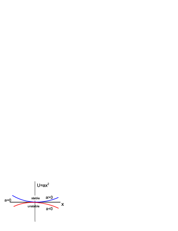
Figure 1: Schematic of the potential energy $U(x)=ax^{2}$ as a function of coordinate $x$ for various $a$: $a>0$, the state with $x=0$ is stable; $a=0$, point of stability loss of the state with $x=0$; $a<0$, stability at $x=0$ is lost.

We shall consider a uniaxial ferroelectric with the ferroelectric axis perpendicular to the film plane, see Fig. 2.

Figure 2: Schematic of the ferroelectric thin film with either dead layers with thickness $d/2$ separating it from the electrodes, or the real electrodes with Thomas-Fermi screening length $\lambda$.

This is the case, for example, of BaTiO₃ (BTO) films compressively strained on SrRuO₃/SrTiO₃ (SRO/STO) substrate. The strained cubic crystal behaves as a uniaxial ferroelectric with second- or weak first-order phase transition. We restrict ourselves here to the case of a second order ferroelectric transition in the bulk, i.e. the Landau-Ginzburg-Devonshire (LGD) free energy density is assumed to have the form:

$$F_{LGD}(P) = \frac{A}{2}P_{z}^{2}+\frac{B}{4}P_{z}^{4}+\ldots+\frac{1}{2}D_{ij}\left(\nabla_{\perp i}P_{z}\right)\left(\nabla_{\perp j}P_{z}\right)$$ (1)

$$+\frac{1}{2}\eta\left(\partial_{z}P_{z}\right)^{2}+\frac{1}{2}\kappa P_{zb}^{2}$$

where $P_{z}$ is the ferroelectric (switchable) component of polarization along the polar axis $z$, $P_{zb}$ is the nonferroelectric part of the polarization along the $z$-axis with $\kappa$ directly related to the so-called background dielectric constant (see the Methodological Note below), $A=A^{\prime}\left(T-T_{c}\right)$ and $A^{\prime},B,$ $D_{ij},$ $\eta,$ $\kappa=\mathrm{const}$, $\nabla_{\perp}=(\partial_{x},\partial_{y})$ the gradient operator in the plane $(x-y)$ of the film. To simplify the formulas, we shall assume that the gradient coefficient is $D_{ij}=D\delta_{ij}$, where $\delta_{ij}$ is the Kronecker symbol. Here, the Landau coefficients are renormalized by the strain produced by the lattice misfit with the substrate $u_{m}$ pertsev98 , see the Appendix D (for BTO on STO $u_{m}=-2.2\%).$

Importantly, we do not include the striction terms that couple strain to $P^{2}$ terms in (1) because they renormalize the $BP_{z}^{4}$ term and this does not affect the loss of stability of symmetric phase in a system like BTO on STO (see below). The point is that, as we said above, finding the loss of stability boils down to solving a linear problem, while this term is nonlinear and does not affect the problem. The statements to the contrary by Pertsev and Kohlstedt in Ref.perkohl07 , that the elastic coupling defines the point of the stability loss and the critical thickness of the FE films, are qualitatively incorrect, as pointed out in Ref. BLcomPer07 . The above form of $F_{LGD\ }$ yields the equation of state for the ferroelectric via standard relation:

$$E_{fz}=\frac{\delta F_{LGD}}{\delta P_{z}}=AP_{z}+BP_{z}^{3}-D\nabla_{\perp}^{2}P_{z}-\eta\partial_{z}^{2}P_{z},$$ (2)

$$E_{fz}=\kappa P_{zb},$$ (3)

which means that the local electric field is in one-to-one correspondence with the local ferro- and nonferroelectric components of the polarization.

II.2 Loss of stability with respect to homogeneous polarization

Since we do not know what type of solutions corresponds to the horizontal line in Fig. 1, we should check all the possibilities. We start by trying the simplest one, a homogeneous change of polarization. This situation is described by the linearized equation of state for a homogeneous polarization $P_{zh}$ (and the nonferroelectric part $\kappa P_{zb}):$

$$E_{fz}=AP_{zh}=\kappa P_{zb}$$ (4)

where $E_{fz}$ is the homogeneous field in the ferroelectric. The dead layer is a linear dielectric, which is described by an equation analogous to (4), hence it is not necessary to consider explicitly the polarization of the dead layer, and we shall describe it by its dielectric constant $\epsilon_{e}$. The boundary condition at the interface of the ferroelectric (continuity of the normal component of the displacement vector) then reads

$$E_{fz}+4\pi\left(P_{zh}+P_{zb}\right)=\epsilon_{e}E_{dz},$$ (5)

where $E_{dz}$ is the field in the dead layer. We can rewrite the above equation as

$$\epsilon_{b}E_{fz}+4\pi P_{zh}=\epsilon_{e}E_{dz},$$ (6)

where $\epsilon_{b}$ is the ”background dielectric constant”, $\epsilon_{b}=1+4\pi/\kappa$. There is also a condition of a zero applied bias (short circuiting, $U=0$):

$$E_{fz}l+E_{dz}d=0.$$ (7)

We find from the above the depolarizing field in the FE film:

$$E_{fz} = -\frac{4\pi d}{\epsilon_{e}l+\epsilon_{b}d}P_{zh}\approx-\frac{4\pi dP_{zh}}{\epsilon_{e}l},$$ (8)

$$E_{dz} = \frac{4\pi l}{\epsilon_{e}l+\epsilon_{b}d}P_{zh}\approx\frac{4\pi P_{zh}}{\epsilon_{e}},$$ (9)

and we see that the field in the dead layer is much stronger than the field in the FE film, $\left|E_{dz}\right|\gg\left|E_{fz}\right|$ because is does not contain the small parameter $d/l\ll 1$, and it is realistic to assume $\epsilon_{b}\sim\epsilon_{e}$. Importantly, the field is concentrated in the dead layers, yet since the layers are very thin, its contribution to the total free energy appears to be negligible (see below). The system of homogeneous equations (4),(8) for $E_{fz}$ and $P_{0}$ has nontrivial solutions only when

$$A=-\frac{4\pi d}{\epsilon_{e}l+\epsilon_{b}d}\approx-\frac{4\pi d}{\epsilon_{e}l}.$$ (10)

This would define the temperature of the stability loss of the paraelectric phase with regards to a homogeneous polarization. It would happen at a lower temperature than the loss of stability of the paraelectric phase in a very thick slab ($l\rightarrow\infty$) or in absence of a dead layer and ideal metallic electrodes ($A=0,$ $T=T_{c}$). Recall that absence of nontrivial solutions at values of $A$ which do not satisfy Eq.(10) means either stability of the solution $P=0$ (the paraelectric phase) or instability of this solution (see Fig.1). and, therefore, stability of another homogeneous solution with $P\neq 0,$ which has to be found from the full, nonlinearized, equation of state. Let us emphasize that this is not necessarily the absolutely stable state but might be a metastable state because we did not consider competing inhomogeneous states which might have a lower energy. Also the temperature defined by Eq.(10) is $not$, in general, the temperature at which the paraelectric phase ceases to exist: one has to consider a loss of stability with respect to an inhomogeneous polarization as well, in order to determine which one sets in first.

Now, consider the case of a finite bias voltage $U$.  In this case, the equilibrium polarization in the paraelectric phase is non-zero, and so are the electric fields in the ferroelectric and the dead layer. One finds

$$lE_{fz}+dE_{dz}=U$$

and, instead of Eq. (8), we obtain the field in the FE film:

$$E_{fz} = E_{0}-\frac{4\pi d}{\epsilon_{e}l+\epsilon_{b}d}P_{zh},$$ (11)

$$E_{0} = \frac{U}{l+\epsilon_{b}d/\epsilon_{e}}\approx\frac{U}{l},$$ (12)

where $E_{0}$ is the external field. The expression for $E_{fz}$ (11) is usually said to mean that the field in the FE film is equal to a sum of the external $E_{0}$ and the depolarizing fields. Substituting Eq. (11) into Eq. (2), we obtain

$$\left(A+\frac{4\pi d}{\epsilon_{e}l+\epsilon_{b}d}\right)P_{0}+BP_{0}^{3}=E_{0},$$ (13)

where $P_{0}$ stands for the equilibrium homogeneous polarization.

Let us check if this equilibrium state can lose its stability with respect to a homogeneous fluctuation of polarization. In textbooks on ferroelectricity, it is shown that when $d=0$ (an ideal metallic electrodes) there is no loss of stability, and the second order transition gets smeared out by the external field. Lets check that the homogeneous transition would also be smeared out in the case of the dead layers. Checking for the stability loss with respect to a homogeneous polarization, we linearize the equation of state (2) near $P=P_{0}$, $E_{fz0}$, where $E_{fz0}$ is the electric field in the ferroelectric in the state with $P=P_{0}$, and obtain

$$\left(A+3BP_{0}^{2}\right)P^{\prime}=E_{fz}^{\prime},$$ (14)

where $P^{\prime}=P-P_{0}$ and $E_{fz}^{\prime}=E_{fz}-E_{fz0}.$ We obtain the same equations for the fluctuation of the polarization $P^{\prime}$ and the field $E_{fz}^{\prime}$ as for the short-circuited case with the only difference that $A$ should be replaced by $\overline{A}=A+3BP_{0}^{2}.$ We have already found [cf. Eq. (10)] that the loss of stability with respect to a homogeneous polarization should take place if

$$\overline{A}=A+3BP_{0}^{2}=-\frac{4\pi d}{\epsilon_{e}l+\epsilon_{b}d}.$$ (15)

This is impossible, however, since from Eq. (13):

$$\overline{A}+\frac{4\pi d}{\epsilon_{e}l+\epsilon_{b}d}=A+\frac{4\pi d}{\epsilon_{e}l+\epsilon_{b}d}+3BP_{0}^{2}=\left(\frac{dP_{0}}{dE_{0}}\right)^{-1},$$ (16)

is always positive. Indeed, $dP_{0}/dE_{0}$ can be considered as the differential susceptibility of a ferroelectric in an external electric field and with the ideal metallic electrodes, but with the coefficient before the $P^{2}$ term equal to $A+4\pi d/\left(\epsilon_{e}l+\epsilon_{b}d\right)$. We have already mentioned that in the case of the ideal metallic electrodes there is no loss of stability and the phase transition is smeared, i.e. $dP_{0}/dE_{0}$ is always positive under a finite bias voltage. We have proven that in a ferroelectric with the dead layers (or real metallic electrodes) the phase transition with respect to the homogeneous polarization is smeared out by an external electric field. As was mentioned above, this does not mean that there is no phase transition. Indeed, there is a possibility that in an external field the film may be losing stability with respect to inhomogeneous polarization. If this takes place, a second order (unsmeared) phase transition occurs  This is why we shall study a loss of stability with respect to the inhomogeneous polarization in a general case of applied external bias voltage.

II.3 Loss of stability with respect to inhomogeneous polarization

Following the same general procedure, we should be looking for a first occurrence of a nontrivial solution to a linearized equation of state that allows for inhomogeneous polarization:

$$E_{z}=\overline{A}P_{z}-D\nabla_{\perp}^{2}P_{z}-\eta\partial_{z}^{2}P_{z}.$$ (17)

Since an inhomogeneous polarization $\widetilde{P}_{z}$ produces an electric field both across the film ($z-$axis) and in perpendicular directions, we should add an equation of state for the two other polarization components. We have:

$$\boldsymbol{P}_{\perp}=\frac{\epsilon_{\perp}-1}{4\pi}\boldsymbol{E}_{\perp},$$ (18)

where $\boldsymbol{E}_{\perp}$ is the in-plane electric field, $\epsilon_{\perp}$ the in-plane dielectric constant. The solution of (17) should also obey the equations of electrostatics:

$$\boldsymbol{\nabla}\times\boldsymbol{E}=0,$$ (19)

$$\boldsymbol{\nabla\cdot}\left(\epsilon_{b}\boldsymbol{E}+4\pi\boldsymbol{P}\right)=0.$$ (20)

Now, we should get inventive. As far as a reasonable solution of equations (17), (19), (20) is concerned, they have a vast set (continuous infinity) of types of solutions and we have to single out only one type of solutions from them that gets realized. We shall apply a physical common sense to restrict the types of the solutions considered. First, the prospective solutions should be periodic in the film plane, since we deal with a large area (practically infinite) film. Any periodic function can be presented as a sum of the sinusoidal functions. Consider the structure that is periodic in the $x$-direction. Then,

$$\widetilde{P}_{z}(x,z)=\sum_{n}\widetilde{P}_{n}\left(z\right)\cos k_{n}x,$$ (21)

where $k_{n}=nk_{1},$ $\widetilde{P}_{n}\left(z\right)$ are the unknown functions and $k_{1}$ is the unknown wavenumber. We have to perform the stability check for arbitrary $k_{1}$. The solution given by Eq. (21) is very complicated, and in reality one does not need to keep all harmonics. It is sufficient to consider the critical harmonic with a one-dimensional periodicity

$$\widetilde{P}_{z}=af\left(z\right)\cos kx,$$ (22)

where $a$ and $k$ are the unknown numbers, $f\left(z\right)$ the unknown function. It adds nothing new if we consider, e.g., $\cos k_{1}x\cos k_{2}y$, because the products of trigonometric functions are the linear combinations of trigonometric functions of other (sum and difference) arguments. Looking among the forms given by Eq. (22), we have already tremendously simplified the problem: for every $k$ we will have a system of ordinary differential equations, instead of a system of partial differential equations. Further, we can identify $f\left(z\right)$ too. First of all, this function should be as smooth as possible. Indeed, the bound charge associated with the inhomogeneous ferroelectric polarization $\rho_{b}=-\boldsymbol{\nabla\cdot P}=a\left(df/dz\right)\cos kx$ should be as small as possible to reduce the electric field energy. It is unreasonable to have $f\left(z\right)=\mathrm{const}$, the bound charge at the ferroelectric-dead layer interface will be proportional to this constant. More reasonable would be to make it nearly constant deep inside the ferroelectric yet smaller at the interface. Taking into account that it should be a solution of a differential equation with the constant coefficients, we are left with an ansatz:

$$\widetilde{P}_{z}=a\cos kx\cos qz,$$ (23)

where $q$ is another unknown parameter, which we expect to be much smaller than $k.$ A critical reader could study other options. It may seem formally possible to try $\cosh qz,$ for example, but this is a bad choice that fails to satisfy the boundary conditions (see below), which are possible to satisfy with Eq. (23).

Using Eq. (17), one obtains for the ansatz (23):

$$\widetilde{E}_{fz}\left(x,z\right)=\left(\overline{A}+Dk^{2}+\eta q^{2}\right)a\cos kx\cos qz.$$ (24)

The electrostatics equation (19)  yields

$$\partial_{z}\widetilde{E}_{fx}=\partial_{x}\widetilde{E}_{fz},$$ (25)

and one finds that

$$\widetilde{E}_{fx}\left(x,z\right)=-\frac{k}{q}\left(\overline{A}+Dk^{2}+\eta q^{2}\right)a\sin kx\sin qz.$$ (26)

Thus, we have found the electric field in the ferroelectric assuming that we have a “polarization wave”. This assumption is consistent if this field satisfies the second electrostatic equation (20), or

$$\epsilon_{b}\partial_{z}\widetilde{E}_{fz}+\epsilon_{\perp}\partial_{x}\widetilde{E}_{fx}+4\pi\partial_{z}\widetilde{P}_{z}=0.$$ (27)

We can easily get rid of $\widetilde{E}_{fx}$ in the above equation by differentiating it with respect to $z$ and using Eq.(25) to obtain

$$\left(\epsilon_{b}\partial_{z}^{2}+\epsilon_{\perp}\partial_{x}^{2}\right)\widetilde{E}_{fz}+4\pi\partial_{z}^{2}\widetilde{P}_{z}=0.$$ (28)

Substituting here the ansatz (24), we find the value of $\overline{A},$ at which the non-trivial solutions are possible as a function of the parameters $k$ and $q$:

$$\overline{A}=-\frac{4\pi q^{2}}{\epsilon_{b}q^{2}+\epsilon_{\perp}k^{2}}-Dk^{2}-\eta q^{2}.$$ (29)

It is still premature to look for a maximum of this function (a point, where the instability sets in first), because we have also (i) to find the fields from the electrostatic equations in the dead layer and (ii) to satisfy the boundary conditions. Given that the field in the dead layer has to have its $z$ component depending on $x$ as $\cos kx$, we put $\widetilde{E}_{dz}=\zeta\left(z\right)\cos kx$ and, therefore, $\widetilde{E}_{dx}=\psi\left(z\right)\sin kx$, where $\psi^{\prime}\left(z\right)=-k\zeta\left(z\right)$. From $\boldsymbol{\nabla\cdot E}=0,$ one has $\zeta^{\prime}+k\psi=0$ or $\psi^{\prime\prime}-k^{2}\psi=0$. Since the transversal component of the electric field is zero at an ideal metallic surface, we find that $\psi\left(z\right)=\Psi\sinh k\left(z-l/2-d/2\right)$ and

$$\widetilde{E}_{dx} = \Psi\sinh k\left(z-l/2-d/2\right)\sin kx,$$ (30)

$$\widetilde{E}_{dz} = -\Psi\cosh k\left(z-l/2-d/2\right)\cos kx,$$ (31)

for $z>l/2.$ The two electrostatic boundary conditions, (i) the continuity of the in-plane electric field component and (ii) the continuity of the displacement, Eq. (5), at the ferroelectric-dead layer interface ($z=l/2$) read

$$a\frac{k}{q}\left(\overline{A}+Dk^{2}+\eta q^{2}\right)\sin\frac{ql}{2}=\Psi\sinh\frac{kd}{2},$$ (32)

$$a\left(\overline{A}+4\pi/\epsilon_{b}+Dk^{2}+\eta q^{2}\right)\cos\frac{ql}{2}=-\frac{\epsilon_{e}}{\epsilon_{b}}\Psi\cosh\frac{kd}{2}.$$ (33)

Excluding $\overline{A}$ from equations (32),(33), with the help of Eq.(29), one finds that this system has a non-trivial solutions for $a$ and $\Psi$ if

$$\frac{q}{\epsilon_{\perp}}\tan\frac{ql}{2}=\frac{k}{\epsilon_{e}}\tanh\frac{kd}{2}.$$ (34)

Since we are interested in the case of thin dead layers, we suppose that $kd\ll 1$. Then, Eq. (34) simplifies to

$$q\tan\frac{ql}{2}=\frac{\epsilon_{\perp}k^{2}d}{2\epsilon_{e}}.$$ (35)

This allows one to exclude $k$ from (35) and (29) and reduce, for the case of thin dead layer, i.e. for $l\gg d\epsilon_{b}/\epsilon_{e},$ $d\eta\epsilon_{\perp}/\left(D\epsilon_{e}\right),$ to:.

$$-\overline{A} = \frac{4\pi d}{\epsilon_{e}l}t(y),\qquad t(y)=y\left(\cot y+r\tan y\right),$$ (36)

$$r = \frac{\epsilon_{e}^{2}D}{\pi\epsilon_{\perp}d^{2}},\qquad y=ql/2.$$ (37)

Now, we can find at what critical thickness of the dead layer the first nontrivial solution appears with $q\neq 0.$ Consider first the case $y=ql/2\ll 1,$ where the function $t(y)\$can be expanded as

$$t\approx 1+\left(r-\frac{1}{3}\right)y^{2}+\left(\frac{r}{3}-\frac{1}{45}\right)y^{4}.$$ (38)

There appears a minimum at $y\neq 0$ for $r<1/3,$ so that the minimal value of $\left|\overline{A}\right|$ is found at $q\neq 0$ for the total thickness of the two dead layers exceeding the critical thickness $d_{m}$:

$$d>d_{m}=\epsilon_{e}\sqrt{\frac{3D}{\pi\epsilon_{\perp}}}$$ (39)

This solution is:

$$q_{c} = \frac{1}{l}\left(15\frac{d-d_{m}}{d_{m}}\right)^{1/2},$$ (40)

$$k_{c} = \left(\frac{5\pi}{\epsilon_{e}}\frac{d-d_{m}}{Dl}\right)^{1/2}.$$ (41)

We see that for $d<d_{m}$ the function $\overline{A}\left(q\right)$ is monotonous and has its maximum value at $q=0$, i.e. for very thin dead layers the phase transition occurs into the homogeneously polarized state. In the case $d\gtrsim d_{m},$ the phase transition occurs into an inhomogeneously polarized state with $k=k_{c}$ given by Eq.(41), i.e. the “wave vector” of the sinusoidal polarization “wave” increases very rapidly from $k=0$ at $d=d_{m}$ to a large value and $ql/2$ rapidly becomes on the order of unity. The corresponding transition temperature is found from

$$|\overline{A}|=\frac{4\pi d}{\epsilon_{e}l}\left(1-\frac{5\left(d-d_{m}\right)^{2}}{4d_{m}^{2}}\right),$$ (42)

i.e. it occurs just slightly above the transition into the homogeneous state, where $|\overline{A}_{h}|=4\pi d/\epsilon_{e}l.$ For BaTiO₃/SrRuO₃ the estimate gives a small value $d_{m}=0.3\mathring{A},$ hence for BTO/SRO such a regime is only of an academic interest, $d\simeq 5d_{m}$ there (see Sec.VI). However, it seems to be very interesting to look for systems where $d_{m}$ may be large, since those systems could perhaps sustain the homogeneous polarization and, therefore, are most interesting for memory applications.

In the opposite limiting case, $d\gg d_{m}$, which is a typical real situation, $ql$ increases and approaches $\pi,$ so that the value of $\tan\frac{ql}{2}$ becomes very large. We suppose that in this case $\epsilon_{\perp}k^{2}\gg\epsilon_{b}q^{2}$ and shall check later that this assumption is justified. Then, one can omit $\epsilon_{b}q^{2}$ in the denominator of the first term on r.h.s. of Eq. (29). Also, the last term can be omitted, because, as we shall see below, the maximum of $\overline{A}$ corresponds to $k\gg q$ and the coefficients $D$ and $\eta$ are normally of the same order of magnitude. Indeed, the maximum of the simplified expression corresponds to

$$k=k_{c}=\left(\frac{4\pi q_{c}^{2}}{\epsilon_{\perp}D}\right)^{1/4}=\left(\frac{4\pi^{3}}{\epsilon_{\perp}Dl^{2}}\right)^{1/4},$$ (43)

since, as we argued above,

$$q_{c}\simeq\pi/l.$$ (44)

In this regime $\epsilon_{\perp}^{1/2}$ $k_{c}/q_{c}=\left(4\epsilon_{\perp}/\pi\right)^{1/4}l^{1/2}/D^{1/4}$. Given that usually $D$ is on the order of magnitude of $d_{at}^{2},$ where $d_{at}$ is the typical interatomic distance (cf. Appendix E) and $\left(4\epsilon_{\perp}/\pi\right)^{1/4}$ is on order of unity, in all real cases one has approximately: $\epsilon_{\perp}^{1/2}k_{c}/q_{c}\simeq\left(l/d_{at}\right)^{1/2},$ i.e. our assumption that $\epsilon_{\perp}k^{2}\gg\epsilon_{b}q^{2}$ for $d\gg d_{m}$ is justified for films thicker than several monolayers.

We see that with increasing thickness of the dead layer $d$ the period of the sinusoidal domain structure rapidly decreases and then saturates at a value independent of $d$. Since at $d-d_{m}=d_{m}$ both Eq. (41) and Eq. (43) give similar values for $k_{c}$ (difference is about $20\%$), the two simple formulas are sufficient to describe the function $k_{c}\left(d\right)$ with a reasonable accuracy at all values of $d$. From Eqs. (43), (44), and (29), one sees that at $d-d_{m}>d_{m}$ the loss of stability of the paraelectric phase with respect to formation of the domain structure takes place at

$$\overline{A}=-2Dk_{c}^{2}.$$ (45)

The relation (29) allows to simplify the expressions for the inhomogeneous fields in the ferroelectric film (24),(26), which we rewrite, using $\epsilon_{\perp}k^{2}\gg\epsilon_{b}q^{2}$, as:

$$\widetilde{E}_{fz}\left(x,z\right) = -a\frac{4\pi^{3}}{\epsilon_{\perp}\left(kl\right)^{2}}\cos kx\cos qz,$$ (46)

$$\widetilde{E}_{fx}\left(x,z\right) = a\frac{4\pi^{2}}{\epsilon_{\perp}kl}\sin kx\sin qz.$$ (47)

Obviously, both fields are much smaller than the magnitude of the polarization wave: since $kl\sim\sqrt{l/d_{at}}\gg 1$, then $\left|\widetilde{E}_{fz}\right|\ll\left|\widetilde{E}_{fx}\right|\ll a.$

In comparison, the field in the dead layers in the studied case $kd\ll 1$ is, near FE interface:

$$\widetilde{E}_{dz}\left(x,z=\frac{l}{2}\right) = a\frac{8\pi^{2}}{\epsilon_{\perp}k^{2}ld}\cos kx$$ (48)

$$= a\frac{4\pi^{1/2}D^{1/2}}{\epsilon_{\perp}^{1/2}d}\cos kx,$$

$$\widetilde{E}_{dx}\left(x,z=\frac{l}{2}\right) = a\frac{4\pi^{2}}{\epsilon_{\perp}kl}\sin kx,$$ (49)

hence, $\widetilde{E}_{dz}$ is much larger than any other field component in the system. As we can see from (48), there is no small parameter like $d_{at}/l$ or $d/l$ in the $z-$component of the field in the dead layer $\widetilde{E}_{dz}$ (the only parameter there is $d_{at}/d,$ $d_{at}\sim D^{1/2}$ [see discussion after Eq.(44)], which is less than unity, yet much larger than the above mentioned other small parameters in the problem.) This is reminiscent of the behavior that we saw above for the case of the homogeneous polarization. These results allow us to construct the maps of the polarization $\widetilde{P}_{z}$ (23) and $\widetilde{P}_{x}=(\epsilon_{\perp}-1)\widetilde{E}_{fx}/4\pi$ characteristic of the sinusoidal polarization distribution, shown in Fig. 3. The map shows the narrow sinusoidal domains with well ordered polarization distribution. The stray electric field component along the film near its surface, $\tilde{E}_{x}$, results in the presence of perpendicular to the easy $z-$axis component of the polarization, $P_{x}$, in the narrow sinusoidal domains. The pattern is similar to the one for the structure with abrupt domains (the well-known Kittel structure with thin domain wallskittel .)

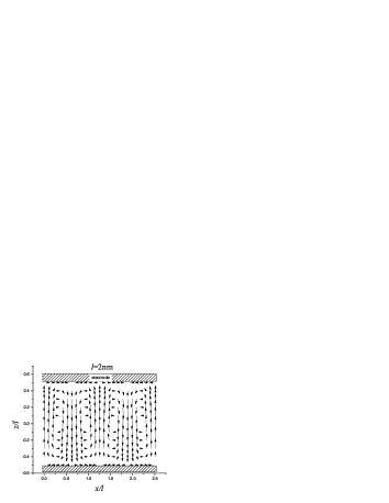
Figure 3: The polarization distribution in the BTO/STO film with thickness $l=2$nm in sinusoidal domain regime. It clearly shows that the electric field component along the film near its surface results in the presence of perpendicular to the easy $z-$axis component of the polarization in the narrow sinusoidal domains. The pattern is similar to the one for the structure with abrupt narrow domains (the Kittel structure).

II.4 Metallic electrode

We would like to compare now the ferroelectric film with the dead layers to the one of real metallic electrodes with Thomas-Fermi screening, in order to see the analogy between the two cases. Obviously, the inhomogeneous polarization in the form (23) will produce the electric field and the electrostatic potential $\varpropto\cos kx,$ so that the electrostatic potential will be $\phi(z,x)=\Phi(z)\cos kx.$ The Poisson equation then takes the form

$$\left(\partial_{z}^{2}-k^{2}\right)\Phi=\Phi/\lambda^{2},$$ (50)

that has the solution $\Phi(z)=-\Phi(-z):$

$$\Phi = \phi_{1}e^{-\kappa(z-l/2)},\qquad z>l/2,$$ (51)

$$\kappa = \sqrt{k^{2}+\lambda^{-2}}.$$ (52)

With this solution, the boundary conditions, found analogously to (32),(33), give:

$$-a\frac{k}{q}\left(\overline{A}+Dk^{2}+\eta q^{2}\right)\sin\frac{ql}{2} = k\phi_{1},$$ (53)

$$a\left(\overline{A}+4\pi/\epsilon_{b}+Dk^{2}+\eta q^{2}\right)\cos\frac{ql}{2} = \frac{\epsilon_{e}}{\epsilon_{b}}\kappa\phi_{1}.$$ (54)

Excluding $\overline{A}$ from these equations with the help of Eq.(29), one arrives at BLapl06 :

$$\frac{q}{\epsilon_{\perp}}\tan\frac{ql}{2}=\frac{k^{2}}{\epsilon_{e}\sqrt{k^{2}+\lambda^{-2}}}.$$ (55)

Considering the case of interest to us, $k\lambda\ll 1,$ and comparing this with (35), we see that for $\epsilon_{\perp}k^{2}\gg q^{2}$ the case of realistic metallic electrodes and the simple dead layer model are mathematically equivalent when $\lambda=d/2.$ Since $d/2$ is the thickness of the dead layer, the result suggests the numerical equivalence of the dead layer and the Thomas-Fermi screening length when $\epsilon_{\perp}k^{2}\gg q^{2}$.

III Properties of a Sinusoidal Domain Structure

Now we turn to the discussion of the ferroelectric phase. It is quite natural to expect that close to the transition the spatial distribution of the polarization may be well represented by a single or a few sinusoids with the wave vector equal to $k_{c}$ in addition to a spatially homogeneous part $p$. There will certainly be a single sinusoidal wave, at least close to the transition, if there is an anisotropy in the ($x-y$) plane. In this review, we discuss this latter case only.

III.1 Range of existence

Consider first a zero external field, $E_{0}=0$, when the homogeneous part of the polarization is zero both in the paraelectric and the ferroelectric phases, i.e. close to the transition there is a single sinusoid and $p=0$. Some distance away from the transition, the single sinusoidal approximation (23) breaks down. Indeed, because of the cubic term in Eq. (2), the polarization of the form $\widetilde{P}=a\cos kx\cos qz$ suggests a presence of an electric field, which depends on the coordinates not only as $\cos kx\cos qz,$ but also as $\cos 3kx\cos qz,$ $\cos kx\cos 3qz,$ $\cos 3kx\cos 3qz.$ Such a field induces polarization containing even higher spatial harmonics, and so forth ad infinitum. Let us estimate when these higher contributions to the field and the higher harmonics in the polarization may be neglected. Suppose that the main part of the polarization is the simplest polarization wave (23). When the polarization is known, one can calculate the electric field produced by this polarization without referring to the equation of state. In our case, it is convenient to use the relation between the polarization and the field at the transition point given by Eq. (28), which yields:

$$\widetilde{E}_{fz} = -\frac{4\pi q_{c}^{2}}{\epsilon_{\perp}k_{c}^{2}}a\cos k_{c}x\cos q_{c}z$$ (56)

$$= -Dk_{c}^{2}a\cos k_{c}x\cos q_{c}z,$$

since $\epsilon_{\perp}k^{2}\gg q^{2}$. It is impossible to satisfy exactly the equation of state (2) with such a field and polarization, and we have to consider the corrections to the field $\check{E}_{z}\left(x,z\right)$: $E_{z}=\widetilde{E}_{fz}+\check{E}_{z}.$ Let us try $\widetilde{P}_{z}$ in the form (23) in (2) to see what is lacking. We obtain:

$$-Dk_{c}^{2}a\cos k_{c}x\cos q_{c}z+\check{E}_{z}\left(x,z\right)$$ (57)

$$= \left(A+Dk_{c}^{2}+\frac{9Ba^{2}}{16}\right)a\cos k_{c}x\cos q_{c}z$$

$$+\frac{Ba^{3}}{16}(3\cos 3k_{c}x\cos q_{c}z$$

$$+\cos k_{c}x\cos 3q_{c}z+\cos k_{c}x\cos 3q_{c}z).$$

One can satisfy this equation by putting

$$A+2Dk_{c}^{2}+\frac{9}{16}Ba^{2}=0,$$ (58)

or

$$a^{2}=-\frac{16}{9}\frac{A+2Dk_{c}^{2}}{B}=-\frac{16}{9}\frac{\widetilde{A}}{B},$$ (59)

and introducing the additional “ghost” fields in order to compensate the rest of the terms on the right hand side. They are not the real electric fields because they do not satisfy the electrostatic equations. In fact, it is inconsistent to take into account the higher harmonics of the field without correcting the polarization self-consistently. But all this trouble is not necessary if those “ghost fields” are small compared to the real ones. The condition for this reads

$$Dk_{c}^{2}>\frac{3}{16}Ba^{2}=-\frac{1}{3}\widetilde{A},$$

or

$$-\widetilde{A}<3Dk_{c}^{2}.$$ (60)

The numerical factor is certainly not reliable and may be omitted.

If the polarization is presented not as a single sinusoid but as a sum of a constant and a sinusoidal parts the condition of neglecting of the higher order harmonics has to be considered anew. In this case, we have close to the phase transition:

$$P_{z}(x,z)=p+a\cos k_{c}x\cos q_{c}z.$$ (61)

For $a,$ we now have from the equation of state,

$$a^{2}=-\frac{16}{9}\frac{A+2Dk_{c}^{2}+3Bp^{2}}{B},$$ (62)

and among the “ghost” fields there is, for example, the component $\frac{3}{4}Bpa^{2}\cos 2k_{c}x\cos 2q_{c}x$ that can be neglected when

$$\frac{4\pi q_{c}^{2}}{\epsilon_{\perp}k_{c}^{2}}>\frac{3}{4}Bpa=Bp\sqrt{-\frac{\widetilde{A}+3Bp^{2}}{B}}.$$ (63)

The maximum of the r.h.s. is at $p=\sqrt{-\widetilde{A}/6B\text{ }},$ so this condition transforms into:

$$-\widetilde{A}<2\sqrt{3}Dk_{c}^{2},$$ (64)

which is practically the same as (60). Let us emphasize that at any temperature the same formula may be applied to describe the states with $p_{c}\lesssim p,$ since the amplitude $a$ cannot be large in this case.

III.2 Free energy

It was convenient and instructive to use the equations of state to describe instability of the paraelectric phase. However, it is more convenient to use a (non-equilibrium) free energy in order to analyze the properties of the sinusoidal domain structures, whose minimization provides us with an equilibrium state. The LGD free energy (1) does not include the energy of the electric field sources, and we shall calculate it now. But first, a simple exercise: let us perform a similar calculation for a linear dielectric with the ideal metallic electrodes at a non-zero voltage $U.$ For simplicity, we assume that the dielectric is extremely anisotropic and has one component of the polarization only, and that only the states with a homogeneous polarization are studied. We have

$$\tilde{F}=\int dV\frac{A}{2}P^{2}+W_{el},$$ (65)

where the integral is taken over the volume of the dielectric and $W_{el}$ is the electric energy. The integrand can be called the LGD free energy for the linear dielectric. The electric energy can be represented as

$$W_{el}=\int dV\frac{E^{2}}{8\pi},$$ (66)

where the integral is now over “the whole universe”, which means in our case over the volume of the dielectric and the voltage source. The latter is imagined as a capacitor with an infinite capacitance. The electric field in the dielectric is always $U/l$ and does not depend on the polarization. When we change the polarization (recall that we consider the non-equilibrium free energy), the charge on the electrodes is changed and, therefore, the charge and the energy of the source are changing too. Suppose first that the polarization is zero and for this state of the dielectric the charge of the source is $Q_{s},$ so its energy is equal to $Q_{s}^{2}/2C$, where $C$ is the capacitance of the source. Consider now a state with the polarization $P.$ The charge on the electrode with the potential $U$ (the second electrode has zero potential by assumption) has then changed by some value $Q$. The electric energy of the source has changed by $\left[\left(Q_{s}-Q\right)^{2}-Q_{s}^{2}\right]/2C=-QU$, where we have taken into account that $U=Q_{s}/C$ and that $Q^{2}/2C\rightarrow 0$ when $C\rightarrow\infty$. In general, the work of the voltage source (change of its energy) can be written as

$$-\sum_{a=1,2}^{\mathrm{electrodes}}e_{a}\varphi_{a} = -(e_{1}\varphi_{1}+e_{2}\varphi_{2})=-e_{1}\varphi_{1}$$ (67)

$$= -QU,$$

where $e_{a}$ are the charges on the electrodes, and we assumed that the second electrodes in earthed. When the polarization is directed outward from the electrode, then the charge on the plate is $Q=PS,$ where $S$ is the electrode (plate) area. Since the electric energy lowers in this case, the equilibrium polarization will be directed from the electrode $U.$ We have proven a well known fact that the polarization tends to be oriented along the field. Now, the full change of the energy per unit area due to a non-zero polarization is $\tilde{F}/S=lAP^{2}/2-PU,$ where $l$ is the thickness of the dielectric plate. Minimizing this non-equilibrium free energy with respect to $P,$ we find $P=\frac{1}{A}\frac{U}{l}.$ This is, of course, a well-known result for a linear dielectric: the equilibrium polarization is directed along the electric field and is proportional to the the field (cf. the standard $P=\chi E)$. Using this, one can find that the sum of the “LGD” energy of a linear dielectric (65) and the energy of electric field inside it at the equilibrium is:

$$\int\left(\frac{A}{2}P_{z}^{2}+\frac{E^{2}}{8\pi}\right)dV=\int\frac{\epsilon E^{2}}{8\pi}dV,$$ (68)

where $\epsilon=1+4\pi\chi,$ which is another well known formula.

Now we can evaluate the free energy of a ferroelectric capacitor at a given bias voltage. Since we are interested in the case of an inhomogeneous ferroelectric polarization, we have to take into account the polarization perpendicular to the polar axis, cf. Eq. (26). For the LGD energy of this polarization together with the energy of the perpendicular electric field in the ferroelectric, we can use Eq. (68). The same is valid for the nonferroelectric part of polarization of the ferroelectric along axis $z$, as well as for the polarization and the electric field of the dead layer. As a result, we obtain a contribution to the full free energy:

$$\int_{FE}\frac{\epsilon_{\perp}E_{\perp}^{2}}{8\pi}dV+\int_{FE}\frac{\epsilon_{b}E_{z}^{2}}{8\pi}dV+\int_{DL}dV\frac{\epsilon_{e}E^{2}}{8\pi},$$ (69)

where the first integral is over the volume of the ferroelectric (FE) and the second over the volume of the dead layer (DL). It is convenient, though not quite consistent, to refer to these contributions as to  the electric field energy

The total energy consists, therefore, of three parts: the LGD contribution, the electric field energy and the energy of the voltage source. It can be presented as (here and below, we will always imply that the free energy is calculated per unit area)

$$\tilde{F} =\int_{FE}dV\Bigl{[}\frac{A}{2}P_{z}^{2}+\frac{B}{4}P_{z}^{4}+\ldots+\frac{1}{2}D_{ij}\left(\nabla_{\bot i}P_{z}\right)\left(\nabla_{\bot j}P_{z}\right)$$

$$+\frac{1}{2}\eta\left(\partial_{z}P_{z}\right)^{2}$$

$$+\frac{\epsilon_{\perp}E_{\perp}^{2}}{8\pi}+\frac{\epsilon_{b}E_{z}^{2}}{8\pi}\Bigr{]}+\int_{DL}dV\frac{\epsilon_{e}E^{2}}{8\pi}-\sum_{a}^{\mathrm{electrodes}}e_{a}\varphi_{a},$$ (70)

where the first integral is over the volume of the ferroelectric (FE) and the second over the volume of the dead layer (DL). At the moment, we want to study an anisotropic film where the polarization changes only along one of the transversal axes (e.g. $x$) and the standard case of $q\ll k$ (see our discussion above). Then, we can simplify the free energy as:

$$\tilde{F} = \int_{FE}dV\Bigl{[}\frac{A}{2}P_{z}^{2}+\frac{B}{4}P_{z}^{4}+\frac{1}{2}D\left(\partial_{x}P_{z}\right)^{2}+\frac{\epsilon_{b}E_{z}^{2}}{8\pi}+\frac{\epsilon_{\perp}E_{x}^{2}}{8\pi}\Bigr{]}$$ (71)

$$+\int_{DL}dV\frac{\epsilon_{e}E^{2}}{8\pi}-QU.$$

Let us mention that the electric field energies for the homogeneous and the sinusoidal parts are additive, as follows from the fact that $\int dx\cos kx=0$ .

Consider the electric field energy for the sinusoidal part. We find from Eqs. (24) and (26), that

$$\widetilde{E}_{fz}\ll\widetilde{E}_{fx}=\frac{4\pi^{2}a}{\epsilon_{\perp}k_{c}l}\sin k_{c}x\sin q_{c}z,$$ (72)

hence, since $\epsilon_{b}$ is hardly larger than $\epsilon_{\perp}$, the energy of the electric field in the ferroelectric is

$$\int\frac{\epsilon_{\perp}}{8\pi}\widetilde{E}_{xf}^{2}dV=l\frac{\pi q_{c}^{2}}{2\epsilon_{\perp}k_{c}^{2}}a^{2}.$$ (73)

We obtain the field in the dead layer from Eq. (32). Recalling that we are interested in the case $kd\ll 1,$ $q\ll k$ and $q\simeq\pi/l,$ we find that in the dead layer:

$$\widetilde{E}_{dx}\ll\widetilde{E}_{dz}=\frac{8\pi^{2}}{\epsilon_{\perp}k_{c}^{2}ld}a\cos k_{c}x=\frac{4\pi^{1/2}D^{1/2}}{\epsilon_{\perp}^{1/2}d}a\cos k_{c}x.$$ (74)

The energy of the electric field in the dead layer is

$$\epsilon_{e}\frac{\widetilde{E}_{dz}^{2}}{8\pi}d\left\langle\cos^{2}k_{c}x\right\rangle=\frac{\epsilon_{e}D}{4\epsilon_{\perp}d}a^{2}=\sqrt{\frac{\pi}{3}}\frac{d_{m}}{d}\frac{D^{1/2}}{4\epsilon_{\perp}^{1/2}}a^{2}.$$ (75)

Taking into account Eqs. (43), (44), one sees that the ratio of the energies of the electric field in the ferroelectric and in the dead layer is $\pi\sqrt{3}d/d_{m},$ i.e. for our case $d\gg d_{m}$ the contribution of the deal layer can be neglected.

Now, it remains to calculate the contribution of the homogeneous part of the electric field energy . To this end, we use Eq. (11) for the electric field in the ferroelectric, find the electric field in the dead layer from Eq. (12), and obtain:

$$W_{el}=\frac{\epsilon_{b}l}{8\pi}E_{fz}^{2}+\frac{\epsilon_{e}d}{8\pi}E_{dz}^{2}=\frac{2\pi p^{2}dl}{l\epsilon_{e}+\epsilon_{b}d}+\frac{\epsilon_{b}\epsilon_{e}U^{2}}{8\pi\left(\epsilon_{e}l+\epsilon_{b}d\right)}$$ (76)

The last term here is the unimportant constant. Finally, the energy of the external voltage source is $-QU$ and for a unit area one finds from Eq. (11):

$$Q=\frac{l}{l+\epsilon_{b}d/\epsilon_{e}}p,$$ (77)

and

$$W_{els}=-\frac{l}{l+\epsilon_{b}d/\epsilon_{e}}pU=-lpE_{0}.$$ (78)

The total electric energy per unit volume equals

$$\frac{\pi q_{c}^{2}}{2\epsilon_{\perp}k_{c}^{2}}a^{2}+\frac{2\pi p^{2}dl}{l\epsilon_{e}+\epsilon_{b}d}-pE_{0}.$$ (79)

Finally, one obtains the LGD contribution to the free energy by using Eq. (61) and calculating the integrals for $q=\pi/l.$ As a result, the free energy per unit area $\tilde{F}(p,a)$ takes the form:

$$l^{-1}\tilde{F}(p,a)=\frac{\tilde{A}+\xi}{2}p^{2}+\frac{\tilde{A}}{8}a^{2}+\frac{B}{4}p^{4}+\frac{3B}{8}a^{2}p^{2}+\frac{9B}{256}a^{4}-pE_{0},$$ (80)

where

$$\widetilde{A} = A+2Dk_{c}^{2},$$ (81)

$$\xi = 4\pi d/\left(\epsilon_{e}l+\epsilon_{b}d\right)-2Dk_{c}^{2}\approx 4\pi d/\left(\epsilon_{e}l\right)-2Dk_{c}^{2},$$ (82)

are the main parameters of the system, $E_{0}=\epsilon_{e}U/\left(\epsilon_{e}l+\epsilon_{b}d\right)\approx U/l$ the external field for the usual case of a thin dead layer $\epsilon_{b}d\ll\epsilon_{e}l.$ The Landau coefficients $A,B,...$ in (1) are renormalized by lattice misfit pertsev98 (see Appendix D), but we do not account for inhomogeneous strain coupled with inhomogeneous polarization in Eq. (71). Its account is irrelevant when one defines the point of stability of the paraelectric phase with respect to the domain formation. Indeed, the coupling between the inhomogeneous polarization and strains is nonlinear, while the problem is linear. This coupling begins to play a role when the finite amplitude $a$ of the “polarization waves” has to be found. Nevertheless, we shall not take it into account to avoid unnecessary complications, which do not change our main conclusions BLcomPer07 .

IV Electric properties of sinusoidal domain structures

IV.1 Polarization - External field curves. Different critical thicknesses for stability loss and for memory

By now, we have made an important step of calculating the free energy of the film with the dead layers in a single harmonic approximation. Already at this level, we can study the regions of (meta)stability of the homogeneous state with respect to domains and determine the corresponding conditions. As we have noted a several times above, the residual depolarizing field in the ferroelectric resulting from an incomplete screening by the electrodes tends to split FE into domains, and that defines the properties of very thin films. Importantly, not only formation but also a response of the domain structure to an external bias voltage appears to be affected by this field by a much greater extent than one might have expectedBLapl06 , as we will discuss below. For instance, the $p-E_{f}$ dependencies have an unusual shape with a negative slope, predicted earlier by the continuum theory for a similar case at low temperaturesBLPRB01 .

Apparently, the thin ferroelectric films are very well suited for an application of the analytical theory of domain structures in ideal crystals. The theory helps to understand some experimental data, as we shall demonstrate in the next Section. However, at the moment this theory is unable to make practical predictions that seem most important, like the estimates of the parameters of the ferroelectric films that may correspond to an acceptable memory performance. This is not surprising, however, since there is no consistent theory of the FE switching.

In this regard, it is worth mentioning that the usual practice of using the Kolmogorov-Avrami approach to describe the switching in FE is very unfortunate. Such an approach was designed for considering nucleation and growth in the absence of any long range interaction between the nuclei, which is far from being the case in the ferroelectrics, and without account for the depolarizing field suppressing creation of isolated nuclei. In other words, strong macroscopic Coulomb interaction defining the behavior of thin films is completely neglected in that approach, and there is no easy way to take it into account. On the other hand, considering domain structures as a superpositions of several sinusoidal distributions of polarization takes consistently into account the Coulomb interaction from the very beginning. Such a superposition is a readily identifiable periodic domain structure for an equilibrium or a metastable state. Considering the switching, one most likely should consider a local perturbation in the periodic structure (nuclei), but it is very inconvenient in terms of the delocalized sinusoidal basis functions. Nevertheless, discussion of thin films with nearly sinusoidal domains gives a possibility to approach the problem of switching from a different perspective. We shall see that even the first step in this direction, i.e. considering purely sinusoidal domain structure with the use of Eq.(80) leads to the non-trivial conclusions. We believe that further description of domain structures in this field is promising and highly desirable.

Here, we present an analysis of the ferroelectric film with the sinusoidal domain structure in the single harmonic approximation and will carefully indicate where this approximation works. By minimizing the corresponding free  energy (80) with respect to $a,$ one finds the equilibrium value of the amplitude:

$$a_{0} = \left[-\frac{16}{9B}\left(\tilde{A}+3Bp^{2}\right)\right]^{1/2}=\frac{4p_{c}}{3^{1/2}}\sqrt{1-s^{2}}\text{ for }\left|s\right|<1,$$ (83)

$$a_{0} = 0\text{ for }\left|s\right|\geq 1,$$ (84)

where $s=p/p_{c},$ with $p_{c}=\sqrt{-\tilde{A}/3B}$ the characteristic polarization. Substituting this solution into Eq.(80) we then arrive at the dimensionless free energy: $f=3B\xi l^{-1}\tilde{F}$ depending on the homogeneous polarization only through the parameter $s$:

$$f_{\pm}(s)=\left\{\begin{array}[]{cc}\frac{1}{2}y\left(1-y\right)s^{2}+\frac{1}{12}y^{2}s^{4}-\sqrt{y}se,&\left|s\right|\geq 1,\\ -\frac{y^{2}}{3}+\frac{y}{2}\left(1+\frac{y}{3}\right)s^{2}-\frac{1}{4}y^{2}s^{4}-\sqrt{y}se,&\left|s\right|<1,\end{array}\right.$$ (85)

where $e=E_{0}/\zeta$ is the relative external field, $\zeta=\xi^{3/2}/\sqrt{3B}$ is the characteristic electric field, and

$$y=-\widetilde{A}/\xi,$$ (86)

is the characteristic temperature (i.e. the relative distance of transition temperature from the paraelectric phase that depends on the film thickness $l$). One can easily see that the free energy is continuous with first derivative with respect to $s,$ while $d^{2}f_{-}/ds^{2}\neq d^{2}f_{+}/ds^{2}$ at $s=\pm 1$.

The equation of state $s=s\left(e\right)$ obtained  from the condition $df/ds=0$ reads:

$$\sqrt{y}\left(1-y\right)s+\frac{1}{3}y^{3/2}s^{3}=e,\qquad\left|s\right|\geq 1$$ (87)

$$\sqrt{y}\left(1+\frac{y}{3}\right)s-y^{3/2}s^{3}=e,\qquad\left|s\right|<1,$$ (88)

and the given state is (meta)stable only when $d^{2}f/ds^{2}>0.$ It is very instructive to compare the behavior of the FE capacitor with real electrodes (or, equivalently, with the dead layers) with that of the system without the dead layers, which does show the standard S-shaped polarization loop described in the dimensionless units by

$$-\sqrt{y}\left(1+y\right)s+\frac{y^{3/2}}{3}s^{3}=e.$$ (89)

We illustrate the behavior of the equation of state depending on the parameter $y$ of the system in Fig. 4. We have selected  different values of $y=1/4,$ $3/2,$ and $3$, corresponding to different temperatures (thus, $y=0$ corresponds to the paraelectric-sinusoidal domain structure transition for $U=0$ occurring at $\tilde{A}=0$, at temperature $T_{d}<T_{c}$), with the results shown in Fig. 4.

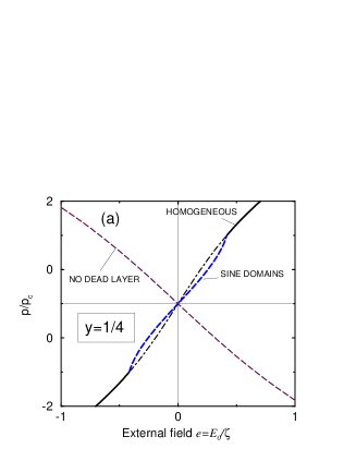
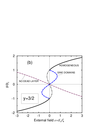
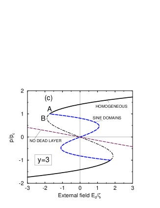
Figure 4: The equation of state $p=p(E_{0})$ for ferroelectric film with dead layer in external field $E_{0}$ for various values of the relative temperature $y$, Eq. (86): (a) $y=1/4$, (b) $y=3/2$, and (c) $y=3$. There is a phase transition between homogeneous state and the one with sinusoidal domains: (a) second order, which becomes first order in cases (b) and (c). All those cases are very different from the case of the FE film without the dead layer. $\zeta=\xi^{3/2}/\sqrt{3B}$ is the characteristic electric field.

We see that at a relatively small $y=1/4$ (for instance, for the system not far below $T_{d}$) the equation of state (87), (88) has only a trivial solution $p=0$ at $E_{0}=0$, i.e. this is the state with no memory. In the field $e>e_{c}=\sqrt{y}-2y^{3/2}/3=5/12$ the system is homogeneously polarized, it splits in the lower bias field via the second order phase transition into domains with zero net polarization in the film at $E_{0}=0.$ At $y=3/2$ (Fig. 4b) this transition is first order (the change of the order of the phase transition occurs at $y=3/8$). This is the first instance when the state with a spontaneous net polarization $p\neq 0$ at $E_{0}=0$ becomes formally possible as a solution to the equations of state. However, this state is unstable ($d^{2}f_{-}/ds^{2}<0$ at $s=\pm 1),$ as is evident from a negative slope of $p-E_{0}$   curve for the upper branch of $f_{-}$ in Fig. 4b.

There is a metastability of a homogeneously polarized state (we shall abbreviate it as the MHS) in the region $3/2<y<3$ [$d^{2}f_{+}/ds^{2}>0$ with the free energy higher than that of the domain state, $f_{+}(\pm 1)>f_{-}(0)$ at $E_{0}=0$]. Formally, both the ferroelectric memory and the polarization switching are possible at these temperatures but no conclusion of practical importance can be made before calculating the escape time from the metastable state. At larger $y\geq 3$ (further down from the phase transition) the state with the homogeneous polarization in the present single-harmonic approximation, Eq. (61), has the same or lower free energy than the state with $p=0,$ $f_{+}(s_{m})\leq f_{-}(0),$ where $\pm s_{m}$ are the positions of the minima of the free energy $f_{+}$ at $E_{0}=0$ (Fig. 5). However, this result is approximate. The reason is that Eq. (23) is valid near the phase transition point only. The region of validity of this approximation has been estimated in chensky82 and above (Sec. IIIA) as roughly $-\tilde{A}<Dk_{c}^{2}$, which means $y\lesssim 1,$ at least for the experimental system BTO on SRO/STO considered below in Sec. V.

In a more accurate approximation accounting for higher harmonics to describe the inhomogeneous polarization, the free energy minimum at $s=0$ dips lower than that of the homogeneous state. It is these higher harmonics that convert the sinusoidal domain structure into a conventional one with narrow domain walls. For the parts of the curves corresponding to $\left|s\right|\gtrsim 1,$ these higher harmonics are not important (they are when amplitude of the first harmonic becomes substantial) but they will change the curves for $\left|s\right|<1$ substantially. The amplitudes of the higher harmonics are to be considered as new variational parameters for the free energy, and their account will be lowering the estimated free energy. Hence, the minimum at $p=0$ in Fig. 5 is actually deeper, and the homogeneously polarized phase becomes stable not at $y=3$ but at a larger value (i.e. at a lower temperature or a larger thickness). Furthermore, it is possible that the homogeneous state would always remain less stable than the polydomain state in that region. Indeed, in the opposite limiting case, i.e. far below the FE transition, it has been shown that for any thickness of the dead layer the multidomain state has a lower free energy than the homogeneously polarized stateBL2000 .

Importantly, the energy barrier between the oppositely polarized states is strongly reduced by the existence of the domain structure at $E_{0}\approx 0,$ Fig. 5. It is very suggestive that one needs to take this into account while considering the problem of polarization switching or the problem of practical memory, but it is a problem that should be dealt separately. We note again that Fig. 4c highlights that homogeneous (single domain) switching is impossible: the homogeneously polarized phase loses its stability with respect to the sinusoidal domain structure at the smaller reverse bias (point A) than the reverse bias flipping the homogeneous polarization (point B). The two (necessarily negative) fields can be calculated from Eqs. (87), (88). One finds the value of $e_{A}$ either Eq.(87) or Eq. (88) for $s=1$:

$$e_{A}=-\frac{2}{3}y^{3/2}+y^{1/2}$$ (90)

The field $e_{B}$ can be obtained from Eq. (87) by extrapolating it to a region $s<1$ and calculating $s$ and $e$ corresponding to the point $de/ds=0.$ One finds,

$$e_{B}=-\frac{2}{3}\left(y-1\right)^{3/2}$$ (91)

We see that the difference between the fields vanishes for $y\gg 1$, but it is appreciable for small values of $y:$ thus, for $y=2$ the difference is about 30%. The applicability of Eqs. (90),(91) is not limited by the region of the one-sinusoidal approximation.

One may ask a question about what happens in a more realistic case where higher powers of $P$ in the Landau expansion, $P^{6}$ or $P^{8},$ may be important, like in BTO on STOBLapl06 . In this case the transition seems to be second order according to first-principles calculationsghosez03 , same as in an earlier parameterization pertsev98 , while the recent parameterizations LiCross05 ; tagBTO07 indicate very weak first order phase transition. A full analysis is fairly involved in the case of more general LGD functional and is beyond the scope of the present work. Nevertheless, the condition for domain instability in a simplest approximation takes the form

$$d^{2}F/dp^{2}=-2Dk_{c}^{2},$$ (92)

where $F$ is the LGD functional for the bulk (or a sample with ideal metallic electrodes) and the second derivative is calculated for $p=p_{e},$ the homogeneous polarization in a given external field $E_{0}$ (this condition will be modified by the strain, but it is reasonable to leave this effect out as a first step). Our analysis indicates that the metastability of the homogeneous state now starts at a smaller $y,$ i.e. closer to the point of the stability loss compared with $y>3/2$ value for the second order case (88). However, since a first order transition occurs before the stability loss, it is not clear if the temperature interval between the transition into ferroelectric phase and appearance of the MHS increases or decreases.

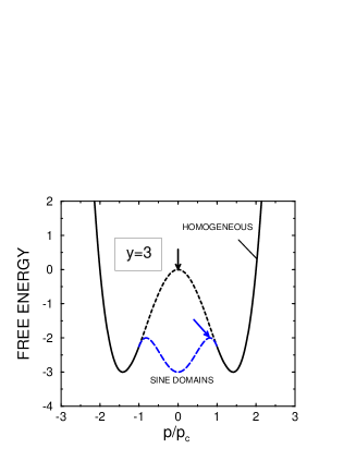
Figure 5: The free energy of the FE film with the dead layer for the relative temperature $y=3$, when the transition between the homogeneously polarized state and sinusoidal domains is first order. It is evident that switching proceeds through the state with domains with much lower energy barrier for nucleation (top of the barriers indicated by arrows). An account for higher harmonics in Eq. (61) will deepen the energy of the domain state compared with the one shown here and will lower the barrier even further.

IV.2 Negative slope of $P(E_{f})$ curves

One unusual property accompanying the domain structure is the negative slope of the $P=P(E_{f})$ curves for ferroelectric films with domain structure. Has been predicted some time ago for ideal films at low temperatures in Ref. BLprlNegEf01 ; BLPRB01 and is viewed as a hallmark of a domain structure governed mainly by electrostaticsBLapl06 . Apparently, this was first experimentally confirmed by the data from Noh et al. KimL05 , who measured the hysteresis loops $P=P(E_{0})$ of ultrathin BTO films on the SRO/STO substrate. It has been very instructiveBLapl06 to replot them as a function of a field in the ferroelectric $E_{f}$, $P=P(E_{f}).$ A remarkable specific feature of replotted loops is that they all have a negative slope, most pronounced at smaller film thicknesses. Certainly, the theory does not give hysteresis loops since its application is limited to an equilibrium state, but the behavior of the equilibrium curve is clearly seen from the dataBLapl06 .

We shall show below that the negative slope of the $P=P(E_{f})$ is characteristic of sinusoidal domain structure near the phase transition. It is worth noting, however, that the negative slope $P/E_{f}<0$ is not an exclusive property of the domain structure. It already happens in the paraelectric phase in the temperature interval $-2Dk_{c}^{2}<A<0,$ where the paraphase is still stable with regards to small inhomogeneous perturbations. To see this for the sinusoidal domain structure, we express the external field through the field in the ferroelectric $E_{f}$ with the use of (11) the additional dimensionless parameter $\psi=1+\xi\left(\epsilon_{e}l+\epsilon_{b}d\right)/4\pi d=\pi d_{m}/\sqrt{3}d$. We obtain:

$$E_{f}=E_{0}-\frac{4\pi dp}{\epsilon_{e}l+\epsilon_{b}d}=E_{0}-\frac{\xi p}{1-\psi}.$$ (93)

To find the response of the sinusoidal domains to the field in the ferroelectric, $dp/dE_{f}$, it is most illustrative to use the equation of state analogous to (88) written in natural units, like

$$\left(-\frac{\widetilde{A}}{3}+\xi\right)p-3Bp^{3}=E_{0},\qquad\left|p\right|<p_{c}.$$ (94)

Now, it is convenient to divide this equation by $Bp_{c}^{3}=-\widetilde{A}p_{c}$ and express $E_{0}$ through $E_{f}$ from Eq. (93). We can then rewrite (88) as

$$\left(\frac{1}{3}-\frac{\psi}{y(1-\psi)}\right)\frac{p}{p_{c}}-\left(\frac{p}{p_{c}}\right)^{3}=\frac{E_{f}}{3Bp_{c}^{3}}.$$ (95)

This yields for the slope at $E_{f}=0:$

$$\frac{dp}{dE_{f}} = -\frac{1}{\widetilde{A}}\frac{3y(1-\psi)}{y\left(1-\psi\right)-3\psi}=\frac{1-\psi}{\xi}\frac{3}{y(1-\psi)-3\psi}$$ (96)

$$= \frac{3\epsilon_{e}l}{4\pi d}\frac{1}{y(1-\psi)-3\psi},$$

where we have used $y=-\widetilde{A}/\xi,$ and $\xi/(1-\psi)=4\pi d/(\epsilon_{e}l+\epsilon_{b}d).$ Finally, this gives for the “dielectric constant” of the ferroelectric film :

$$\epsilon_{f}=1+4\pi dP/dE_{f}=\frac{3\epsilon_{e}l}{d}\frac{1}{y(1-\psi)-3\psi}.$$ (97)

At the point of stability loss with respect to sinusoidal structure, the dielectric constant is already negative, as we mentioned above:

$$\epsilon_{f}=-\frac{3\epsilon_{e}l}{d\psi}=-\frac{4\pi}{2Dk_{c}^{2}}=-l\sqrt{\frac{\epsilon_{\perp}}{\pi D},}$$ (98)

This result is, of course, identical to the standard value of the “dielectric constant” of the FE film itself

$$\epsilon_{f}^{\mathrm{para}}=1+\frac{4\pi P}{E_{f}}\approx\frac{4\pi}{A}=-\frac{4\pi}{2Dk_{c}^{2}}<0,$$ (99)

at the border of stability loss into sinusoidal domain structure. Note that the negative sign of $\epsilon_{f}$ does not mean an instability, because this coefficient does not characterize the response of the system as a whole to an external field, which is $E_{0},$ not $E_{f}.$ The capacitance of the device is defined as a response to $E_{0}$ that is always positiveBLPRB01 .

One can see that the slope becomes positive at $y>3\psi/(1-\psi)$, yet this result is beyond domain of applicability of the single-harmonic approximation. In fact, we know that the slope is negative for the film with domains at low temperatures, as has been predicted some time agoBLPRB01 : it is a hallmark of domain structure governed mainly by electrostatics. Indeed, a net polarization of the domain structure is $\bar{P}=0$ in zero external field $E_{0}$. At small $E_{0}$ there will be positive net polarization in external field because of growth of domains oriented along the external field, and the resulting negative field in the FE. Thus, the “dielectric function” of the film is negative, $\epsilon_{f}=1+4\pi d\bar{P}/dE_{f}|_{E_{f}=0}<0$ BLPRB01 . Comparing theory with the data, the expression for the “dielectric constant”, given by Eq. (31) of Ref. BLPRB01 , can be simplified to

$$\epsilon_{f}\approx-\epsilon_{e}l/d.$$ (100)

Substituting the numbers for the BTO on SRO/STO film with thickness $l=5$nm, we find the theoretical value $\epsilon_{f}=-525$ for equilibrium conditions while the experimental one found from Fig. 61b (raw data for $2$kHz, Ref. KimAPL05 ) is $\epsilon_{f}=-680$, i.e. both estimated and measured values are pretty close. The slope is negative in all samples with thicknesses up to 30nm studied in Ref. KimL05 , see Fig. 7.

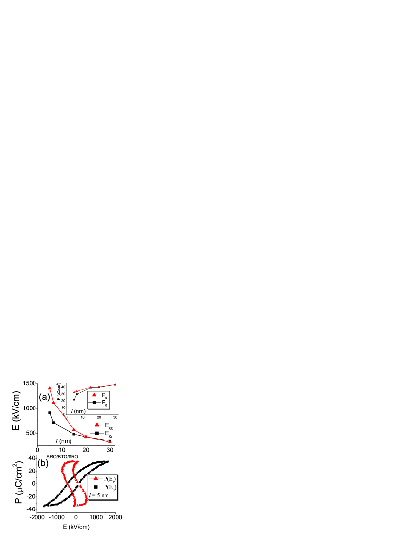
Figure 6: (a) The external field $E_{0b}$ (where $E_{f}=0$) and $E_{0r}$ where the relaxation of polarization starts in 5 nm thick filmKimL05 . Inset: the spontaneous polarization $P_{s}$ and the extrapolated $P_{0}$KimL05 . (b) The measured $P(E_{0})$ and the “actual” $P(E_{f})$ hysteresis loops.

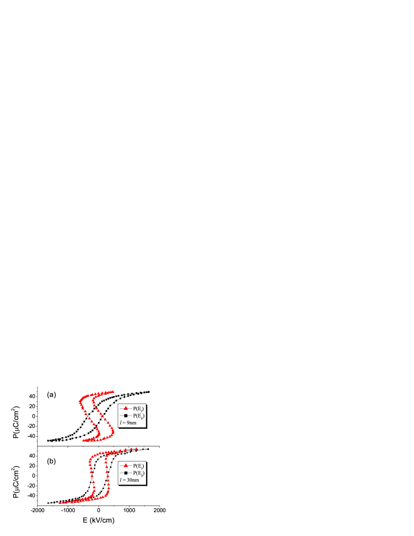
Figure 7: The measured $P(E_{0})$ and the “actual” $P(E_{f})$ hysteresis loops: (a) film thickness $l=9$ nm, (b) $l=$30 nm.

V Experimental example: BaTiO₃ films with SrRuO₃ electrodes on SrTiO₃ substrate

Our above assumption of a second order phase transition may be a reasonable approximation for BaTiO₃ films on SrRuO₃/SrTiO₃ (BTO/STO) substrate that have been investigated down to thickness $l=5$nmKimL05 ; KimAPL05 ; nohNodl06 . We use it to illustrate our theoretical results while discussing, in particular, the effects of the higher order terms in the LGD free energy. Because of $-2.2\%$ lattice mismatch, the BTO film effectively becomes a uniaxial FE and can be treated within the Landau-Ginzburg-Devonshire (LGD) free energy very accurately (results are precisely the same as in ab-initio calculations where the latter are availableBLapl06 .)

Our aim is to describe what we think to be a consistent method of interpreting the experimental data, i.e. the ferroelectric hysteresis loops for the BaTiO₃ films on SrRuO₃/SrTiO₃ with different thicknesses, from $5$ to $30$nm. The electrode parameters were found to be KimL05 : $d/2=\lambda=0.8$Å, $\epsilon_{e}=8.45$. The parameters of the material, i.e. the LGD coefficients for the homogeneous states are taken from LiCross05 with a renormalization due to the lattice misfit strain and the clamping according to pertsev98 , see the Appendix A. This set is different from the one used in Ref.pertsev98 and there are qualitative differences in some experimentally verifiable conclusions for the two sets. In particular, the coefficients of LiCross05 imply a weak first order paraelectric-ferroelectric phase transition, while those of pertsev98 imply a second order one, which is also suggested by the results of the first-principles modelingghosez03 . Since the definitive experimental studies were not carried out, it is not clear which set is better, and we have chosen to use the set of Ref.LiCross05 , when discussing homogeneously polarized state, but the assuming second order phase transition while treating the domain structures.

What remains undefined are the additional boundary conditions (ABC) parameters, but we show below that they can be neglected in the case of BTO on SRO/STO. This can be seen from the analysis of the experimental data for single domain states. The role of the ABC for homogeneously polarized states has been studied in many papers in the present geometry when the polar axis is perpendicular to the film plane, starting with Kretschmer and Binder Kretschmer . Specific features of a ferroelectric surface/interface have been taken fully into account only recentlyBL05 . For a symmetric system (two identical surfaces) and single domain state their effect is reduced to a renormalization of the coefficient $A,$ similar to that of Ref. Kretschmer $A\rightarrow A_{1}=A+\left(2\alpha+\beta\right)/l$, where $\alpha$ and $\beta$ are the parameters pertaining to a surface/interface. One can find the polarization directly from the experiment which would correspond to a zero external field, $E_{0}=0,$ if there were no domains. In Ref. KimL05 it has been found by extrapolation of the high external field part the $p\left(E_{0}\right)$ curves to $E_{0}=0.$ Generalizing Eq. (13) to account for the ABC and the higher order terms in the LGD free energy, we obtain:

$$\left(A_{1}+\frac{4\pi d}{l\epsilon_{e}}\right)p+Bp^{3}+Cp^{5}+Fp^{7}=E_{0},$$ (101)

i.e. for $E_{0}=0$

$$A_{1}+\frac{4\pi d}{l\epsilon_{e}}+Bp_{0}^{2}+Cp_{0}^{4}+Fp_{0}^{6}=0,$$ (102)

and one can find $A_{1}\left(l\right)$ from the experimental data for $p_{0}\left(l\right)$. The equation for spontaneous polarization $P_{s}$ (polarization in the film with zero internal field, $E_{f}=0$):

$$A_{1}+Bp_{s}^{2}+Cp_{s}^{4}+Fp_{s}^{6}=0,$$ (103)

and find it as a function of $l$. Since we know from the data the polarization at zero external field, $p_{0}=p(E_{0}=0)$KimL05 , we can easily obtain $p_{s}$ from (102),(103). The functions $p_{e0}\left(l\right)$ and $p_{s}\left(l\right)$ are shown in Fig.6(inset). We see that the dependence $p_{s}\left(l\right)$ is weak, i.e. the ABC can be ignored, since the variation of the spontaneous polarization $P_{s}$ with thickness due to the $(2\alpha+\beta)/l$ term is small, and we shall assume $A_{1}=A.$

Let us now discuss what the theory tells about the state of films of different thickness at $E_{0}=0$. Let us consider first the case of $B>0.$ This case has been discussed in Sec. IV. We shall start with this case and then try to generalize it. From Eq. (101) for $E_{0}=0,$ one sees that the solution $p=0$ (the paraelectric phase) becomes the only possibility at $l<4\pi d/\left(-A\epsilon_{e}\right).$ Using the above value for the coefficient $A,$ we find that it happens at $l=l_{h}=3.5$nm.

However, we also need to study the stability of the paraelectric and homogeneously polarized state with respect to the domain formation. First, we calculate the value of critical dead layer $d_{m}$ for our system. The value of the transversal dielectric constant, $\epsilon_{\perp},$ can be calculated with the use of the LGD coefficients, and we find that $\epsilon_{\perp}=218$ at room temperature (Appendix D). Then, using Eq. (39), we find that $d_{m}=0.34$Å, i.e. in our case $d=5d_{m}.$ Using values of $\lambda,\epsilon_{e}$ from Ref. KimL05 , calculating $\epsilon_{\perp}$ using the coefficients of Ref. LiCross05 (Appendix D), and the value of $\sqrt{D/4\pi}=0.2$Å from Ref.shirane2 (Appendix E), we obtain the following critical thickness for domains at room temperature ($\epsilon_{\perp}=218)$:

$$l_{d}^{\text{RT}}=\left(\frac{\pi D}{\epsilon_{\perp}}\right)^{1/2}/|A|\simeq 1.6\text{ nm.}$$ (104)

Since $d>d_{m}$, then $l_{d}^{\text{RT}}<l_{h}^{\text{RT}}$, and the phase transition is into a multidomain state. The spatial distribution of a spontaneous polarization is near sinusoidal at $l\gtrsim$ $l_{d}^{\text{RT}}$. Higher harmonics develop with increasing thickness, and the polarization distribution tends to a conventional structure with narrow domain walls. The half-period of the sinusoidal domain structure can be estimated as $a_{c}=1.7$ nm at the transition and as $a^{\text{RT}}=2.2$nm for $l=5$nm from $a\approx\pi/k_{c}$ and (45).

It is instructive to consider the phase transition with regards to the thickness at zero temperature, where we get $\epsilon_{\perp}=408,$ $l_{d}^{(0\text{K)}}=0.8\mathrm{nm}$, $l_{h}^{(0\text{K)}}=2.5$nm. The last result (a homogeneous critical thickness of $2.5$nm) is remarkable, since it practically coincides with the ab-initio calculation for the critical thickness of $2.4$nm in Ref.ghosez03 . The ground state of the film is, however, not homogeneous but multidomain, and the domain ferroelectricity appears in films thicker than $l_{d}^{(0\text{K)}}=0.8$nm, which is the true “critical size” for ferroelectricity in FE films in the present study at zero temperature.

To use the results of Sec. IV, it is convenient to express the variable $y$ as a function of the film thickness. Since $2Dk_{c}^{2}\propto l^{-1},$ one can put $2Dk_{c}^{2}\left(l\right)=l_{c}2Dk_{c}^{2}\left(l_{c}\right)/l=-Al_{c}/l.$ Then $\widetilde{A}\left(l\right)=A-Al_{c}/l=A\frac{l-l_{c}}{l}$. The parameter $\xi\left(l\right)=4\pi d/\left(\varepsilon_{g}l+\epsilon_{b}d\right)-2Dk_{c}^{2}\left(l\right)$ can be obtained as follows. The phase transition into the homogeneous state would occur at $l=l_{h}$, at $A+4\pi d/\left(\epsilon_{e}l_{h}+\epsilon_{b}d\right)=0$ (Sec. IIB). Therefore, $A=-4\pi d/\epsilon_{e}l_{h}$, hence $4\pi d/\left(\epsilon_{e}l+\epsilon_{b}d\right)\simeq$ $4\pi d/\epsilon_{e}l=-Al_{h}/l$ and $\xi=-Al_{h}/l+Al_{c}/l=-A\left(l_{h}-l_{c}\right)/l$. Finally, we get $y=\left(l-l_{c}\right)/\left(l_{h}-l_{c}\right)$. We see that the beginning of the memory for the case of a second order transition from the paraelectric phase, which is at $y=3/2,$ corresponds to $l=4.5$nm. Recall that for this case the homogeneous phase becomes stable at $y>3$ (or for $l>7.3$nm) within our approximation, but this conclusion is unreliable because, as we discussed above, the homogeneously polarized state will almost certainly remain metastable.

Returning now to the experimental data for BTO on SRO/STO, we should mention that the thinnest film ($5$nm) is thicker than the academic “limit for memory” even if $B>0$ and even more so for $B<0.$ This does not mean, however, that the sample has a real stable memory because apart from the memory loss because of absolute instability of the homogeneously polarized state there is also a memory loss because of domain nucleation. There is still no reliable theory of this process, but we can gain some insight into the process by analyzing the experimental data. No memory has been found with a lifetime longer than 1 second in BTO on SRO/STO capacitors with thicknesses less than 30nmKimL05 . Kim et al have found that during the observation time $t_{relax}=10^{3}$s the domains begin to form only if the applied external field along the polarization is less than $E_{0r}=910$kV/cm for 5nm sample (raw data). We can immediately estimate from the results above that at $E_{0}=E_{0r}$ the domains begin to form only when there is a field in the film $E_{f}=-\left(490\pm 70\right)~{}$kV/cm opposite to the polarization. This is natural: it was known for a long time that in order to nucleate domains one has to apply an “activation field” $\left(E_{a}\right)$Merz56 . Studying relatively thick BaTiO₃ samples with $l=\left(2.5-35\right)\times 10^{-3}$cm, Merz Merz56 found that this field depends both on the waiting time $\tau$ and on the sample thickness $l$ and have obtained an empirical formula for it:

$$E_{a}=\left(\alpha\ln\tau\right)/l.$$ (105)

In his thick samples, Merz identified the activation fields to be up to $20$ kV/cm, which looks quite high if one were to apply the Merz’s scaling law (105) to Noh’s samples KimL05 . Indeed, the thicknesses of the films in Ref. KimL05 are four orders of magnitude smaller, while the fields are less than the two orders of magnitude larger. It is evident that the Merz’s formula cannot be applied literally to the films of all thicknesses. (To be fair, Merz studied not the strained BaTiO${}_{3},$ but this hardly accounts for such a difference). However, within the interval of thicknesses studied in Ref. KimL05 the Merz’s formula describes, at least qualitatively, the dependence of the activation field on the film thickness (see Fig.6). It is worth mentioning that at small thicknesses the domain structure is nearly sinusoidal, and one can expect weaker pinning compared to thicker films. It is hardly surprising that the empirical Merz’s formula obtained for conventional domain structure does not apply to a sinusoidal one.

Using Eq. (101), one can find that the electric field in short-circuited sample is about $1200$ kV/cm, exceeding the magnitude of the estimated activation field. This means that in a short-circuited sample single domain state relaxes faster (perhaps much faster) than in $10^{3}$s. If the value of the activation field is defined by the thickness only and not by properties of electrodes or an electrode-film interface, one can speculate about the properties of electrodes that can facilitate a smaller field in a short-circuited sample and a longer, at least $10^{3}$s, retention of a SD state. We have found that for $l=5$nm such an electrode should have $\lambda/\epsilon_{e}=d/2\epsilon_{e}<0.043$Å. Indeed, with such a hypothetical electrode the depolarizing field in an unbiased 5nm sample would be less than 500 kV/cm discussed above. Since in the BTO samples KimL05 the value $\lambda/\epsilon_{e}$ is about $0.1$Å, it does not seem totally impossible to find such an electrode. This will correspond to $d=0.73$Å$\approx 2d_{m}$, the phase transition would be still into a multidomain state. The homogeneously polarized state that is metastable at $l_{h}=1.4$nm would be retained for at least $10^{3}$s in the 5nm BTO film with such an electrode according to the discussion above. One can estimate the critical thicknesses for the domain states to see that here too $l_{d}<l_{h}$ (since $d>d_{m}),$ although the estimates should use more accurate formula for $k_{c},$ compared to (43), because $d$ is getting close to $d_{m}.$ While looking for possibilities for ferroelectric memories, it seems more promising to optimize both the properties of the electrode and the FE material. Recall that $d_{m}\propto D^{1/2}$ and the constant $D$ proved to be particularly low for the (100) orientation of BaTiO₃ shirane2 . From a theory viewpoint, we see that one can play with electrodes, materials, orientations of the film growth, and the misfit strains to find a combination that may be suitable for the nanosize ferroelectric memory elements.

VI Conclusions

We have described the application of the Landau theory to a problem of (meta)stability of a homogeneous state in thin ferroelectric films. The theory allows to better understand the data and gain more insight into the practically important problem of memory (meta)stability in thin films. One advantage is that the theory can start with relatively simple ground state. We have proven, in particular, that switching of a polarization necessarily goes via the intermediate domain state, the empirical fact well known from experiment. The emerging domain structures in thin films are quite unusual, the “sinusoidal” ones. We show the distribution of the polarization, which is reminiscent of the one for domains with abrupt distribution of polarization (the Kittel structurekittel .) To slow down the polarization relaxation into a domain state, one can select different electrodes or ferroelectrics, and the theory guides one as to what parameters are favorable. For instance, ferroelectrics with large energy of domain walls (large gradient, or inhomogeneous terms in the free energy) should have better memory retention.

There are many open questions for both theory and experiment. For instance, there is no acceptable theory of the polarization switching as of yet and, therefore, theory cannot predict what parameters are needed to achieve a needed memory retention. How the sinusoidal domains evolve with temperature and/or thickness of the film into the standard domains with sharp domain walls, remains to be investigated. Obviously, the continuous theory will play very important role in this future work.

APL has been partially supported by Spanish MEC (MAT2006-07196) and CICYT NAN-2004-09183-C10-07.

Appendix A Historical note

The mathematical equivalence of electrostatics and magnetostatics led, at the beginning of development of  the theory of ferroelectric domain structure, to applying the relevant results of the theory of magnetic domain structures to the case of ferroelectrics. The ferromagnetic domains were postulated by Weiss in 1907. However, until 1935 their origin had not been actually understood. Several authors tried to understand their origin within statistical mechanics of an infinite medium. This was even the case with such an outstanding scientist as F.Bloch,Bloch curiously, in the same paper where he considered the famous “Bloch domain wall”. In 1935 Landau and Lifshitz LL35 pointed out futility of these efforts and indicated the demagnetizing effect of surfaces as the origin of ferromagnetic domains, i.e. the demagnetizing field existing in finite magnetic bodies. Landau and Lifshitz proposed a fairly complete theory of ferromagnetic domain structure and obtained some formulas which since then were often attributed to other authors. For instance, the proportionality of the width of the domains to the square root of a film thickness $l$ is frequently attributed to Kittel (see also LL8 ). Kittel highly appreciated the Landau and Lifshitz work and has further developed their theory in 1940’s summarizing the Landau and Lifshitz’s and his own results in his often cited review kittel . For later development of the ferromagnetic domain theory see, e.g., a textbook Hubert .

In the theoretical part of their pioneering paper on the domain structure of Rochelle salt and KH₂PO${}_{4},$ Mitsui and Furuichi mitsui pointed out the relevance of the earlier results for ferromagnets with strong uniaxial anisotropy to their case. Also in 1950’s the group of Känzig Kanzig clearly realized that the depolarizing field in ferroelectrics should be much more important than in ferromagnets. They argued that in a slab of an uniaxial ferroelectric, e.g. KH₂PO₄, with the polar axis perpendicular to the slab plane no phase transition into mono-domain state is possible and the only possibility of phase transition into ferroelectric phase is with formation of a domain structure. This phase transition should occur at a lower temperature and the lowering of temperature is inversely proportional to the slab thickness. They tried to estimate this lowering of the phase transition temperature to find what is now called ”the critical thickness for the ferroelectricity” in the case of KH₂PO₄. They also clearly understood that their estimates are irrelevant to the case of a three-axial ferroelectric such as BaTiO₃ where the closure domains (nowadays called “vortices”) should form. The possibility of screening of the depolarizing field not only by free charges from the electrodes but also by the charge carriers of the material itself was also clearly realized at the very beginning of a systematic study of ferroelectricity. One can see the relevant discussion, in e.g. papers by the group of Känzig Kanzig .

Ivanchik Ivanchik considered the possibility of a mono-domain state in a slab of nonelectroded uniaxial ferroelectric taking into account the screening of the depolarizing field by the carriers of the material, which was treated as a semiconductor with a large band gap. Later he and others Ivanchik et al. took also into account the screening by metallic and semiconductor electrodes. Also in 1960s, the effect of finite screening length of metallic electrodes on dielectric measurements has been discussed by several authors Mead61 ; Ku64 ; Simmons65 . Batra and Silverman BatraSil criticized some details of an approach adopted by Ivanchik’s group and considered an effect of incomplete screening by the electrodes on the phase transition into the ferroelectric state assuming that the phase transition proceeds into a mono-domain state. This topic was later developed in a series of papers by Batra et al.Batra et al. . Similar to the Ivanchik’s group, the main assumption of two series of paper, stability of the mono-domain state was never checked although earlier Bjorkstam and Oettel Bjorkstam pointed out that incomplete screening due to a near electrode dead layer may lead to the same domain structure as in non-electroded samples. It is clear now that the assumption about a monodomain state is almost never satisfied for realistic parameters of the systems, at least close to the phase transition. Chensky Chensky substantially improved the Känzig’s group determination of lowering of a phase transition temperature due to impossibility of transition into a monodomain state in a nonelectroded slab of a ferroelectric with the polar axis perpendicular to the slab. Selyuk considered screening of the depolarizing field by both space and surface charges and found that below the phase transition a monodomain state may become energetically more favorable than the multi-domain one Selyuk .

The next important step was the Chensky and Tarasenko paper mentioned in the Introduction. Recently, the Chensky-Tarasenko approach to study different cases of the domain structure formation at phase transitions has been used by Bratkovsky and Levanyuk BLinh02 and by Stefanovich et al.Stefanovich for the case of phase transition in ferroelectric periodic structures. Some other papers are cited in the main text. The depolarization field screening due to charge carriers of the material and those of the electrodes has been recently reconsidered by Watanabe Watanabe . He obtained results substantially different from those of the Ivanchik’s group at the expense of making several important mistakes, he also avoided any comparison of his results with those of the previous authors.

This historical note does not pretend to represent an exhaustive review of development of theory of the domain structures in ferroelectrics. We have not mentioned many important works aiming at citing only the most important ones falling into the scope of the present paper. In particular, we did not mention many papers devoted to domain structures far from the phase transition (one could call this case the ”Kittel limit” versus the ”Chensky-Tarasenko limit”) as well as papers related to ferroelastic domains. Although conceptually the latter topic is close to the theory of 180-degree domains formation considered in this paper, it is still well beyond its scope.

Appendix B Additional boundary conditions

The equation of state (2) relates electric field at a given point not only to the polarization at the same point but also to its spatial derivatives. In the electrodynamics of continuous media this is referred to as an account for spatial dispersion of dielectric constant LL8 , Agranovich . Differential equations of the electrodynamics with account for the spatial dispersion are of higher order than in usual (”local”) electrodynamics, i.e. to specify among solutions of these equation those that correspond to physical situation one needs more boundary conditions than in the local electrodynamics. These are the “additional boundary conditions” (ABC). Their origin for different physical systems is discussed in detail in Agranovich .

Another way to ABC consists in applying the Landau theory of phase transitions not to an infinite medium but to finite systems. For the first time such an approach has been proposed in the paper by Ginzburg and Landau GL50 , where the Landau theory has been used, in particular, to analyze properties of thin superconducting films. The authors argued that at the boundary superconductor-vacuum or superconductor-dielectric the derivative of the order parameter along the normal to the surface should be zero in the absence of a magnetic field. With such boundary conditions there is no dependence of the phase transition temperature on the film thickness. As far as we know, the first example of the phase transition temperature dependent on the film thickness was given by Ginzburg and Pitaevsky GinzburgPit , who considered superfluid phase transition in thin films of liquid helium sandwiched between two solids. They argued that the order parameter should be zero at liquid helium-solid interface. The influence of this boundary condition can be easily understood considering the loss of stability of the normal phase in the same way as in the present paper. Replacing in Eq. (1) $P_{z}$ by $\eta$ one obtains the free energy of the Landau theory of phase transitionsLLStatphys . Since in the case of superfluid transition there is no physical field conjugated to the order parameter instead of Eq. (17) one has

$$A\eta-g\partial_{z}^{2}\eta=0,$$ (106)

with the boundary conditions $\eta\left(z=\pm l/2\right)=0$, where $l$ is the film thickness. Since at $A>0$ the solutions of this equation are real exponentials, no non-trivial solution satisfies the boundary conditions and the normal phase is stable. At $A<0,$ it has a solution $\cos\left(\sqrt{-A/g}z\right)$ which satisfies the boundary conditions, if $\sqrt{-A/g}l=\pi$. This value of $A$ corresponds to the loss of stability of the normal phase, i.e. the phase transition takes place at $A\left(T=T_{cf}\right)=-\pi^{2}g^{-1}l^{-2}.$ Within the Landau theory $A=A^{\prime}\left(T-T_{cb}\right),$ where $T_{cb}$ is the bulk transition temperature. Therefore, $T_{cf}-T_{cb}\propto-l^{-2}.$

In 1960s, there was an intensive discussion of  the ”proximity effects”, i.e. the properties of a system consisting of a normal metal deposited on top of a superconducting metal. For the superconductor film the main effect was the lowering of the phase transition temperature. At the end, it has been realized that for sufficiently thick layers of the two materials and in the absence of magnetic field this effect can be described within the Ginzburg-Landau theory, i.e. the Landau theory for superconductors completed by the boundary conditions:

$$\lambda\frac{d\eta}{dz}\pm\eta=0,$$ (107)

for $z=\pm l/2,$ where $l$ is the thickness of the superconductor film sandwiched between layers of a normal metal and $\lambda$ is the parameter of the interface, the so-called extrapolation length. Boundary conditions of this form were proposed by de Gennes deGennes while considering another system, the Josephson junction, while their general character was understood by Zaitsev Zaitsev . These de Gennes-Zaitsev boundary conditions Deutscher proved to be applicable well beyond the theory of superconductivity and were derived later on for many different systems.

For $\lambda>0$, the only case considered by de Gennes and Zaitsev, the phase transition in the film occurs again at a lower temperature than in the bulk. Indeed, the  solution of  Eq. (106) is again $\cos\left(\sqrt{-A/g}z\right)$ but to satisfy the boundary conditions the value of $A$ should satisfy the equation

$$\tan\left(\kappa_{1}l/2\right)=\frac{1}{\lambda\kappa_{1}},$$

where $\kappa_{1}=\sqrt{-A/g}.$ For $l\gg\lambda,$ the solution of this equation is $A\simeq-\pi^{2}g^{-1}\left(l+\lambda\right)^{-2}$ and, therefore, the form of distribution of the order parameter at the phase transition point is $\cos\left[\pi z/\left(l+\lambda\right)\right],$ and this functional form explains the term ”extrapolation length”.

Later, these conditions appeared in study of ferromagnets derived from purely phenomenological point of view by Kaganov and Omelyanchuk Kaganov . These authors have taken into account dependence of the surface energy of the crystal on the order parameter via terms $\alpha\eta^{2}\left(\pm l/2\right)/2$ in the free energy per unit surface considering ferromagnetic phase transition in a slab with the anisotropy axis in the slab plane. In this geometry, no magnetic field arises due to inhomogeneous magnetization. As a result, they have arrived at the condition

$$g\frac{d\eta}{dz}\pm\alpha\eta=0,$$ (108)

which is the same condition as Eq. (107). The most important novelty of Ref.Kaganov is that a possibility of the two signs of $\lambda=g/\alpha$ (”positive and negative surface energy”) has been discussed. In the case of negative $\lambda,$ a non-trivial solution is possible at $A>0$. It is $\cosh\left(\sqrt{A/g}z\right),$ which satisfies the boundary conditions if

$$\tanh\left(\kappa_{2}l/2\right)=\frac{1}{\lambda\kappa_{2}},$$

where $\kappa_{2}=\sqrt{A/g}$. For $l\gg\left|\lambda\right|,$ this equation has the solution $\kappa_{2}=\left|\lambda\right|^{-1},$ i.e. at $A=g\lambda^{2}.$ We need to mention that now the phase transition occurs at $A>0$ and the temperature of the transition is independent of $l$, i.e. the same transition would occur at the surface of an infinite half-space. The form of distribution of the order parameter at the transition is characterized by exponential fall-off of the order parameter while going from the surface into the bulk, i.e. the phase transition is now not a bulk but a surface transition. The width of the region affected by the transition increases approaching the temperature of the transition in the bulk, so that all the results for the film are to be affected by the transition. For an infinite half-space, this occurs at $A=0$ only. Of course, the Kaganov-Omelyanchuk treatment is valid also for ferroelectrics with the polar axis lying in the slab plane as well as for any order parameter which is not coupled with long-range fields.

Kretschmer and Binder Kretschmer , while using the same boundary conditions, have taken into account that for ferromagnets and ferroelectrics with the magnetization (polarization) perpendicular to the surface the surface effect will be affected by magnetic (electric) field arising due to the inhomogeneities in the magnetization (polarization). For ferroelectrics, their case is that of a slab with short-circuited ideal metallic electrodes, i.e. of a transition into single-domain state. They found essential differences with the case of absence of the depolarizing field, i.e. they found essential differences between the cases of polarization parallel and perpendicular to the surface. Tagantsev and Guerra Tagantsev have demonstrated recently that in this problem one needs to take into account the noncritical part of the polarization. We shall follow them in this regard.

Along with a modified Eq.(106), which has now the form

$$AP-g\partial_{z}^{2}P=E,$$ (109)

one has to consider an electrostatics equation

$$\partial_{z}\left(\epsilon_{b}E+4\pi P\right)=0,$$

or

$$E+\frac{4\pi}{\epsilon_{b}}P=C=\frac{4\pi}{\epsilon_{b}l}\int_{-l/2}^{l/2}Pdz,$$ (110)

where the constant $C$ is found from the condition of the short circuit: $\int_{-l/2}^{l/2}Edz=0$. Substituting Eq.(110) into (109) one obtains

$$\left(A+4\pi/\epsilon_{b}\right)P-g\partial_{z}^{2}P=C,$$

and has to look for a non-trivial solution of this equation satisfying the boundary conditions (107). The form of the solution does not depend now on the sign of $A$, it is

$$P=\frac{C}{A+4\pi/\epsilon_{b}}+C_{1}\cosh\kappa z,$$

where $\kappa=\sqrt{\left(A+4\pi/\epsilon_{b}\right)/g}$ and $C_{1}$ is another constant related to $C$ via Eq. (110). As a result, one finds

$$P=\frac{C}{A+4\pi/\epsilon_{b}}\left(1+\frac{A\kappa l}{2\sinh\left(\kappa l/2\right)}\cosh\kappa z\right).$$

The boundary conditions (107) are satisfied if

$$A = -\frac{2}{\kappa l\left(\lambda\kappa+\coth\left(\kappa l/2\right)\right)}\simeq-\frac{2}{\kappa l\left(\lambda\kappa+1\right)}$$ (111)

$$= -\frac{2\alpha}{\kappa l\left(g_{1}\kappa+\alpha\right)}.$$

Since $\kappa^{-1}$is the same order of magnitude as the interatomic distances, the approximation in this equation is very good. The polarization distribution at the transition is

$$P\propto 1-\frac{\alpha}{\left(g\kappa+\alpha\right)\sinh\left(\kappa l/2\right)}\cosh\kappa z.$$ (112)

One sees that now the phase transition occurs in the whole volume, both for a ”hard”, $\alpha>0,$ and for a ”soft”, $\alpha<0$, with the polarization that is practically constant over the volume being somewhat smaller for ”hard” surfaces and somewhat larger for the soft ones. The shift of the phase transition temperature in the both cases is proportional to $l^{-1}$.

Since $\kappa^{-1}$is very small, the formulas for the polarization distribution near ferroelectric surfaces are beyond the continuous medium theory used by Kretschmer and Binder and should be considered as qualitative. In this sense account for the noncritical polarization is not very essential here. Another shortcoming of their theory mentioned above is overlooking the “polar” character of a surface which is not important for ferromagnets but is essential for ferroelectrics. This importance has been emphasized by Levanyuk and Minyukov LevMin . While discussing surface structural phase transitions, these authors have pointed out that when $\eta$ can be identified with polarization perpendicular to the surface, the de Gennes-Zaitsev boundary conditions should be complemented by an additional term which makes them inhomogeneous. Bratkovsky and Levanyuk BL05 have explicitly taken into account the complete boundary conditions considering phase transition in a slab of uniaxial ferroelectric with ideal metallic electrodes. Because of the inhomogeneity of the boundary conditions, the polarization is never zero over all the volume, even in the paraelectric phase, though the region where it is not zero is the same as the near-surface region in the Kretschmer and Binder theory, i.e. its thickness is comparable to interatomic distances. Still, to study stability of the paraelectric phase one has to linearize the problem not with respect to $P=0,$ but with respect to $P_{e}\left(z\right),$ an inhomogeneous distribution existing in the paraelectric phase. As a result, instead of Eq.(109) for $P$ one has an equation for $\delta P=P-P_{e}\left(z\right)$ with the coefficient of the first term $A+BP_{e}^{2}\left(z\right)$ instead of $A$ in Eq.(109). This means an additional ”hardening” of the surface layer or an effective positive renormalization of the coefficient $\alpha$ calculated in Ref. BL05 . This means, e.g., that a surface which is ”soft”, $\alpha<0,$ for polarization parallel to the surface, may be ”hard” with respect to polarization perpendicular to the same surface. The polarity of surfaces leads also to smearing of the phase transition if the two surfaces are different BL05 .

Here, we have given only a very brief overview of the phenomenological theory of the surface effect on ferroelectric phase transitions leaving aside both microscopic theories and discussion of other effects of the surfaces, e.g. their role in the polarization switching (see Tagantsev1 ). In 1990s, when thin ferroelectric films became a popular topic there appeared numerous papers reconsidering the phenomenological theory and trying to find its parameters from the experimental data or microscopic theories. We shall not review these papers because, to our understanding, they did not advanced much the development of the phenomenological theory in comparison with the papers cited above. This certainly true of the formulation of the boundary conditions and finding the phase transition temperature that we were concerned about in this Appendix.

We do not take into account the ABC in the present review. From the point of view of electrodynamics of continuous media, this is allowed since the ”spatial dispersion of the dielectric constant” is taken into account in the direction parallel to the surface ($x$) and, in effect, not in the direction perpendicular to the surface ($z$): the coefficient $g$ does not enter our final formulas. Physically, this is justified by the rigidity of polarization with respect to its variation along $z-$axis, which we have discussed while reviewing the results of Kretschmer and Binder. In addition, the experimental data for the system (BTO on STO/SRO) we have used to illustrate the theory indicates that the ABC can be neglected BLapl06 .

Appendix C Methodological note

There is a lot of confusion in the literature with regards to the formula for the energy of a ferroelectric with account for both the voltage source and the electric field due to the polarization of the material. That is why we preferred to use the equations of state as long as possible and, when being forced to consider the free energy, we demonstrate its correctness by comparing the results obtained from the equations of state and from minimization of the free energy. By the way, the trouble with the Watanabe’s papers Watanabe mentioned in the Historical note is due to his use of the free energy while the Ivanchik’s group used the equations of state to treat the same problem.

To begin with, we note that some authors write the LGD functional as a function of $\boldsymbol{P}$ while others did it as function of the dielectric displacement $\boldsymbol{D}.$ The first group includes Ginzburg Ginzburg , Devonshire Devonshire , Jona and Shirane Jona , as well as many others, e.g. Batra et al. and the present authors. The second group includes importantly Lines and Glass Lines and, e.g. Ivanchik et al.Ivanchik , Ivanchik et al. . There is also the third group led by Tagantsev Tagantsev86 , Tagantsev who pointed out that in some situations it is important to take into account that the order parameter does not refer to the total polarization but only to a part of it and there is also another ”background” or ”noncritical” contribution. In some problems it should be taken into account when the effects of depolarizing field are considered. In this review, unlike in our previous works, we have taken it into account but it proved out that it disappears from the final results for the problems that we considered here, which is not necessarily the case for some other problems.

We think that the origin of existence of these variations in the functional representations is the Landau and Lifshitz book ”Electrodynamics of Continuous Media” published in the USSR in 1957 and translated into English in 1960 Landauelectr . This excellent book had a mishap of using $\boldsymbol{D}$ instead of $\boldsymbol{P}$ exactly in the section devoted to ferroelectrics. It has been eliminated in the second edition of the book LL8 , at least partially, but, because, perhaps, of a great authority of Landau, the confusion originated.

The reason why Landau and Lifshitz put what we call now the LGD thermodynamic potential as a function of $\boldsymbol{D}$ is that the equilibrium thermodynamic properties of a system in a presence of an external voltage source are described by thermodynamic potential depending on $\boldsymbol{D}.$ This reasoning is flawed, however, because the thermodynamic potential (or free energy) of the Landau theory of phase transitionsLLStatphys is a non-equilibrium thermodynamic potential (free energy). It depends on the order parameter apart from the conventional thermodynamic variables and only after minimization with respect to the order parameter and substitution of its equilibrium value into the original formula one obtains the equilibrium thermodynamic potential. The order parameter describes the structural changes in the material leading to the breaking of symmetry, which is the central idea of this theory. In the case, of e.g. cubic-tetragonal phase transition in BaTiO₃ this structural change consists mainly in shift of the Ti ion with respect to the Ba sublattice. Of course, the O ions also displace but to change the symmetry from cubic to tetragonal the shift of Ti ions is sufficient. Equally, a shift of only O ions without a shift of Ti ions would lead to the same symmetry breaking. This illustrates the statement that in the Landau theory the physical meaning of the order parameter does not matter but only its symmetry properties. For ferroelectrics, this is emphasized in the book by Strukov and Levanyuk Strukov and is correct while the effects of the depolarizing field are not considered. Quite often, it makes no difference whether to use $\boldsymbol{P}$ or $\boldsymbol{D}$ within the region of applicability of the ”orthodox” Landau theory, i.e. for small values of the order parameter and not far from the phase transition. It is known, in particular, that in ferroelectrics normally $\boldsymbol{P}\gg\boldsymbol{E}$, i.e.$4\pi\boldsymbol{P}\simeq\boldsymbol{D}.$ However, even close to the phase transition one has to take into account that the physical order parameter represents structural changes with respect to which the system loses its stability at the transition, while considering effects of the depolarizing field. In the case of proper ferroelectrics, these structural changes can be related to a polarization but not necessarily to the full polarization of the crystal. At the same time, it is the latter which enters the electrostatics equations. This can make it necessary to take into account the ”background dielectric constant”, which is an independent phenomenological constant not entering the ”orthodox” Landau expansion, to be determined from the experimental data or from the microscopic theory.

We see that much care is needed while applying the LGD theory to discuss different phenomena in ferroelectrics. The examples where the proper care was not taken are too numerous to be discussed here. One can say only that the book by Strukov and Levanyuk Strukov can be improved in this regard. As an illustrative example, recall the boundary condition for the order parameter imposed by Ivanchik Ivanchik who considered a homogeneously polarized ferroelectric slab with a depolarizing field screened by the charge carriers of the material. The electrostatics dictates that the value of $D_{n}$, should be zero at the surface. Since Ivanchik considered $D_{n}$ as the order parameter entering the LGD functional he was forced to conclude that the order parameter is zero at the surface. But what does it mean? That the Ti or O ions in the surface layer are forced to stay in the same positions as in the cubic phase? Nonsense. These ions can be shifted, of course, but in such a way that at the surface $D_{n}=0.$ This is clearly seen if one considers $P_{n}$ as the order parameter. One concludes that at the surface $E_{n}=-4\pi P_{n}$ but these quantities are not necessary zero and what are their values is a separate question. If one takes into account the background dielectric constant ($\epsilon_{b}$) one obtains $E_{n}=-4\pi P_{n}/\epsilon_{b},$ which does not change the qualitative result but may be important for numerical estimations. Batra and Silverman BatraSil (see Historical note) were right in their criticism of Ivanchik’s boundary condition in spite of considering a case where this condition is not necessary and where using either $P_{n}$ or $D_{n}$ as the order parameter makes no difference, and it is also not necessary to take into account $\epsilon_{b}.$

There are several equivalent forms of writing down the free energy of ferroelectric taking into account electric field created by the polarization itself and by external voltage source in the cases where there is no other source of the field rather than the ferroelectric polarization (like in a non-electroded ferroelectric slab) or there is no electric field outside of the ferroelectric and the voltage source (like in a ferroelectric slab with the ideal metallic electrodes). We shall not discuss these forms here because we are interested in a more general case. Let us mention only that a careless generalization to this case of one of the above-mentioned formulas leads quite often to errors, which could be avoided if the authors were to compare at least some of their results with those obtained from the system of equations of state and equations of electrostatics. Obviously, the equations of state usually generate much less controversy than the forms of the free energy.

In the present review, we use nearly the same formula for the free energy as Chensky and Tarasenko chensky82 , with the only difference in writing a noncritical polarization term. They did not discuss the origin of their formula but we shall explain why we think it is quite natural. Conceptually, it follows the same line as, e.g. the calculation of energy of collective excitations accompanied by long-range (electric or magnetic) fields Agranovich . First, one considers these excitations without any long-range fields as if these fields were compensated by external charges or currents, the so-called ”mechanical excitons”. Then, one adds the energy of the long-range field created by the exciton without an account for the changes, which such fields could produce in the exciton itself, i.e. as if the fields were created in vacuum by the bound charges or the Ampere currents of the ”mechanical exciton”. In our case, the “mechanical” part for the ferroelectric energy is given by Eq.(1), which does not contain any electric field and $P$ in this formula has to be considered as a purely structural parameter. There is of course also a ”mechanical” noncritical part of the dead layer. The both have the form of the first term of the LGD formula (with another coefficient, of course), because we do not take into account neither nonlinearities (the second term) nor the spatial dispersion (the third and the fourth terms) in the noncritical dielectric properties and in those of the dead layer. It is shown in the text, see Eq.(68), that the sum of the two energies, the ”mechanical” and the ”purely electric” ones, gives what is used to be called the “energy of electric field in a dielectric”. If we had considered explicitly a real metallic electrode, which we avoided for simplicity sake, we would be obliged to take into account not only the energy associated with the displacements of its atoms and deformations of the filled electronic shells (the ”background dielectric constant”), but also an energy associated with redistribution of electrons in the conduction band, while calculating the ”mechanical”energy of the electrode. This part is quite often overlooked but a detailed discussion of this question would take too much space to do it here.

Appendix D Landau parameters for strained BaTiO₃

The Landau parameters entering the equation of state of perovskite BaTiO₃ film on SrRuO${}_{3}/$SrTiO₃ entering Eq.(2) are found from the parameters for the bulk BTO LiCross05 under conditions of homogeneous in-plane misfit strain $u_{m}=(a-a_{0})/a_{0}=(b-b_{0})/b_{0}=-0.022$:

$$A=2a_{3}^{\ast},\quad B=4a_{33}^{\ast},\quad C=6a_{111},\quad F=8a_{1111},$$ (113)

where

$$a_{3}^{\ast}=a_{1}-u_{m}\frac{2Q_{12}}{s_{11}+s_{12}},\quad a_{33}^{\ast}=a_{11}+\frac{Q_{12}^{2}}{s_{11}+s_{12}}.$$ (114)

The dielectric function in direction along the film $\epsilon_{\perp}=1+\left(2\epsilon_{0}a_{1}^{\ast}\right)^{-1}$, where $a_{1}^{\ast}=a_{1}-u_{m}\left(Q_{11}+Q_{12}\right)/\left(s_{11}+s_{12}\right)$ pertsev98 . When the strain drives transition second order from the weak first order, one can approximate the dielectric function in a direction along the easy axis $z$ and $P_{z}\equiv P_{3}$ (perpendicular to the film plane) as $\epsilon_{c}=1+\left(4\epsilon_{0}\left|a_{3}^{\ast}\right|\right)^{-1}$. The bulk BTO parameters appearing above are (in SI units): $a_{1}=4.124\times 10^{5}(T-115)\quad$C^-2m²N, where $T$ is the temperature in ^∘C, $a_{11}=-2.097\times 10^{8}\quad$C^-4m⁶N, $a_{111}=1.294\times 10^{9}\quad$C^-6m¹⁰N, $a_{1111}=3.863\times 10^{10}$C^-8m¹⁴N, $Q_{11}=0.10,$ $Q_{12}=-0.034,$ $Q_{44}=0.029$ (C^-1m²) yamada72 . The components of the compliance tensor for BTO are $s_{11}=8.3\times 10^{-12},$ $s_{12}=-2.7\times 10^{-12},$ and $s_{44}=9.24\times 10^{-12}$ (in units of m²N^-1).

Here in the text we are using the standard CGS units instead of the SI units, and the quantity we need to make estimates is the (dimensionless in CGS) first Landau coefficient $A=\epsilon_{0}A_{\text{SI}}=-0.0054$, $\epsilon_{\perp}=218$ at room temperature. The coefficient $A_{\text{SI}}$ is found from (113),(114) and other relations given above.

Appendix E Gradient term for BaTiO₃

The gradient coefficient $D$ for BaTiO₃ was estimated from the neutron scattering data shirane2 in the following way. The experimental data gives the dependence of the soft mode frequency on the wave vector for the directions perpendicular to (100). In terms of the present paper, the soft mode frequency in the paraelectric phase can be obtained from the polarization dynamic equation:

$$m\frac{d^{2}P_{\boldsymbol{k}}}{dt^{2}}+\left(A+Dk^{2}\right)P_{\boldsymbol{k}}=0,$$ (115)

where $m$ is a coefficient which will be determined, and $\boldsymbol{k}$ is the wave vector in the plane perpendicular to (100). Then,

$$\omega^{2}\left(k\right)=\frac{A+Dk^{2}}{m}.$$ (116)

We have found the coefficient $m$ from the value for $\omega\left(0\right),$ and then estimated from the rest of the curve $\sqrt{\epsilon_{0}D_{\text{SI}}}=0.17$Å ($D_{\text{SI}}$ is the gradient term in SI units, the same estimate as we gave in Ref.BLapl06 ). In the CGS units, used in the present paper, the value is $\sqrt{D/4\pi}=0.17$Å.

References

- (1) L.D. Landau and E.M. Lifshitz, Phys. Z. Sowjet. 8, 153 (1935).
- (2) C. Kittel, Rev. Mod. Phys. 21, 541 (1949)
- (3) T. Mitsui and J. Furuichi, Phys. Rev. 90, 193 (1953).
- (4) L.D. Landau and E.M. Lifshitz, Electrodynamics of Continuous Media (Butterworth Heinemann, Oxford, U.K., 1980), Sec 44.
- (5) A.M. Bratkovsky and A.P. Levanyuk, Phys. Rev. Lett. 84, 3177 (2000).
- (6) A.M. Bratkovsky and A.P. Levanyuk, Phys. Rev. Lett. 87, 179703 (2001).
- (7) A.M. Bratkovsky and A.P. Levanyuk, Phys. Rev. B 63, 132103 (2001).
- (8) A.M. Bratkovsky and A.P. Levanyuk, Phys. Rev. B 66, 184109 (2002).
- (9) C. Jaccard, W. Kanzig, and M. Peter, Helv. Phys. Acta 26, 521 (1953).
- (10) E.V. Chensky and V.V. Tarasenko, Sov. Phys. JETP 56, 618 (1982) [Zh. Eksp. Teor. Fiz. 83, 1089 (1982)].
- (11) S. K. Streiffer, J. A. Eastman, D. D. Fong, C. Thompson, A. Munkholm, M.V. Ramana Murty, and O. Auciello, Phys. Rev. Lett. 89, 067601 (2002).
- (12) A.M. Bratkovsky and A.P. Levanyuk, cond-mat/0601484.
- (13) A.M. Bratkovsky and A.P. Levanyuk, Appl. Phys. Lett. 89, 253108 (2006).
- (14) D.J. Kim, J.Y. Jo, Y.S.Kim, Y.J. Chang, J.S. Lee, J.-G. Yoon, T.K. Song, and T.W. Noh, Phys. Rev. Lett. 95, 237602 (2005).
- (15) Y.S. Kim, D.H. Kim, J.D. Kim, Y.J. Chang, T.W. Noh, J.H. Kong, K. Char, Y.D. Park, S.D. Bu, J.-G. Yoon, and J.-S. Chung, Appl. Phys. Lett. 86, 102907 (2005).
- (16) Y.S. Kim, J.Y. Jo, D.J. Kim, Y.J. Chang, J.H. Lee, T.W. Noh, T.K. Song, J.-G. Yoon, J.-S. Chung, S. I. Baik, Y.-W. Kim, and C.U. Jung, Appl. Phys. Lett. 88, 072909 (2006).
- (17) A.M. Bratkovsky and A.P. Levanyuk, arXiv: 0708.3273v1 (2007).
- (18) R. Kretschmer and K. Binder, Phys. Rev. B 20, 1065 (1979).
- (19) A.M. Bratkovsky and A.P. Levanyuk, Phys. Rev. Lett. 94, 107601 (2005).
- (20) N.A. Pertsev, A.G. Zembilgotov, and A.K. Tagantsev, Phys. Rev. Lett. 80, 1988 (1998).
- (21) N.A. Pertsev and H. Kohlstedt, Phys. Rev. Lett. 98, 257603 (2007).
- (22) A.M. Bratkovsky and A.P. Levanyuk, arXiv: 0709.4256v1 (2007).
- (23) J. Junquera and P. Ghosez, Nature 422, 506 (2003).
- (24) Y.L. Li, L.E. Cross, and L.E. Chen, J. Appl. Phys. 98, 064101 (2005).
- (25) Y.L. Wang, A.K. Tagantsev, D. Damjanovic, N. Setter, V.K. Yamarkin, A.I. Sokolov, and I.A. Lukyanchuk, J. Appl. Phys. 101, 104115 (2007).
- (26) J. Harada, J.D. Axe, and G. Shirane, Phys. Rev. B 4, 155 (1971).
- (27) W. Merz, J. Appl. Phys. 27, 938 (1956).
- (28) T. Yamada, J. Appl. Phys. 43, 328 (1972).
- (29) F. Bloch, Z. Phys. 74, 295 (1932).
- (30) A. Hubert and R. Schäfer, Magnetic Domains (Springer, Berlin, 1998).
- (31) C. Jaccard, W. Känzig, and M. Peter, Helv. Phys. Acta 26, 521 (1953); M. Anliker, H.R. Bruger, and W. Känzig, ibid, 27, 99 (1954).
- (32) I.I. Ivanchik, Fiz. Tverd. Tela, 3, 3731 (1961) [Sov. Phys.-Solid State, 3, 2705 (1962)]
- (33) G.M. Guro, I.I. Ivanchik, and N.F. Kovtonyuk, Fiz. Tverd. Tela, 11, 1956 (1969) [Sov. Phys.-Solid State, 11, 1574 (1970)]; B.M. Vul, G.M. Guro, and I.I. Ivanchik, Fiz. Tekh.Poluprov. 4, 162 (1970) [Sov.Phys. Semicond. 4, 128 (1970)].
- (34) C.A.Mead, Phys. Rev. Lett. 6, 545 (1961).
- (35) H.Y. Ku and F.G. Ullman, J. Appl. Phys. 35, 265 (1964).
- (36) J.G. Simmons, Appl.Phys.Lett. 6, 54 (1965).
- (37) I.P. Batra and B.D. Silverman, Sol. State Commun. 11, 291 (1972).
- (38) I.P. Batra, P. Wurfel, and B.D. Silverman, Phys. Rev. Lett. 30, 384 (1973); I.P. Batra, P. Wurfel, and B.D. Silverman, Phys. Rev.B 8, 3257 (1973); P. Wurfel and I.P. Batra, Phys.Rev. B 8, 5126 (1973).
- (39) J.L. Bjorkstam and R.E. Oettel, Phys. Rev. 159, 427 (1967).
- (40) E.V. Chenskii, Fiz. Tverd. Tela, 14, 2241 (1972) [Sov.Phys.-Solid State 14, 1940 (1973)].
- (41) B.V. Selyuk, Kristallografiya 16, 356 (1971).
- (42) V.A. Stephanovich, I.A. Luk’yanchuk, and M.G. Karkut, Phys. Rev. Lett.94, 047601 (2005).
- (43) Y. Watanabe, J. Appl. Phys. 83, 2179 (1998); Phys. Rev. B 57, 789 (1998).
- (44) V.M.Agranovich and V.L.Ginzburg, Crystal Optics with Spatial Dispersion, and Excitons (Springer, Berlin, 1984).
- (45) V.L.Ginzburg and L.D.Landau, Zh.Eksp. Teor.Fiz. 20, 1064 (1950) [In: Collected Papers of L.D.Landau, edited by D. ter Haar, (Gordon and Breach, London,1965), p.546.]
- (46) V.L.Ginzburg and L.P.Pitaevsky, Zh. Eksp. Teor.Fiz. 34, 1240 (1958) [Sov.Phys. JETP 7, 858 (1958)].
- (47) L.D.Landau and E.M.Lifshitz, Statistical Physics (Butterworth-Heinemann, Oxford, 1980).
- (48) P.G. de Gennes, Phys. Letters 5, 22 (1963).
- (49) R.O. Zaitsev, Zh. Eksp. Teor.Fiz. 48, 1759 (1965) [Sov. Phys. JETP 21, 1178 (1965)].
- (50) G.Deutscher and P.G. de Gennes, In: Superconductivity, edited by R.D.Parks, (Dekker, New York, 1969),p.1005; P.G. de Gennes, Superconductivity of Metals and Alloys (Benjamin, New York, 1966).
- (51) M.I. Kaganov and A.N. Omelyanchuk, Zh. Eksp. Teor.Fiz. 61, 1679 (1971) [Sov. Phys. JETP 34, 895 (1972)].
- (52) A.K. Tagantsev and G. Gerra, J. Appl. Phys. 100, 051607 (2006).
- (53) A.P.Levanyuk and S.A. Minyukov, Fiz. Tverd. Tela, 25, 2617 (1983) [Sov.Phys.-Solid State 25, (1983)].
- (54) G. Gerra, A.K. Tagantsev, and N. Setter, Phys. Rev. Lett. 94, 10762 (2005).
- (55) V.L. Ginzburg, Zh. Eksp. Teor.Fiz. 15, 739 (1945) [Journ. Phys. USSR 10, 107 (1946)]; Zh. Eksp. Teor.Fiz. 19, 36 (1949); Usp. Fiz.Nauk. 38, 490 (1949) (in Russian).
- (56) A. Devonshire, Phil. Mag. 40, 1040 (1949); 42, 1065 (1949); Adv. Phys. 3, 85 (1954).
- (57) F. Jona and G. Shirane, Ferroelectric Crystals (Pergamon, Oxford, 1962).
- (58) M.E. Lines and A.M. Glass, Principles and Applications of Ferroelectrics and Related Materials (Clarendon, Oxford, 1977)
- (59) A.K. Tagantsev, Ferroelectrics 69, 321 (1986).
- (60) L.D. Landau and E.M. Lifshitz, Electrodynamics of Continuous Media (Pergamon, Oxford 1960).
- (61) B.A. Strukov and A.P. Levanyuk, Ferroelectric Phenomena in Crystals (Springer, Berlin, 1998).