Sparse Fourier Transform via Butterfly Algorithm

Abstract

We introduce a fast algorithm for computing sparse Fourier transforms supported on smooth curves or surfaces. This problem appear naturally in several important problems in wave scattering and reflection seismology. The main observation is that the interaction between a frequency region and a spatial region is approximately low rank if the product of their radii are bounded by the maximum frequency. Based on this property, equivalent sources located at Cartesian grids are used to speed up the computation of the interaction between these two regions. The overall structure of our algorithm follows the recently-introduced butterfly algorithm. The computation is further accelerated by exploiting the tensor-product property of the Fourier kernel in two and three dimensions. The proposed algorithm is accurate and has an $O(N\log N)$ complexity. Finally, we present numerical results in both two and three dimensions.

Keywords. Fourier transform; Butterfly algorithm; Multiscale methods; Far field pattern.

AMS subject classifications. 65R99, 65T50.

1 Introduction

We consider the rapid computation of the following sparse Fourier transform problem. Let $N$ be a large integer and $X$ and $K$ be two smooth (or piecewise smooth) curves in the unit box $[0,1]^{2}$. Suppose $\{x_{i},i\in I\}$ and $\{k_{j},j\in J\}$ are, respectively, the samples of $NX$ and $NK$, where $NX:=\{N\cdot p,p\in X\}$ and $NK$ is defined similarly. Given the sources $\{f_{j},j\in J\}$ at $\{k_{j},j\in J\}$, the problem is to compute the potentials $\{u_{i},i\in I\}$ defined by

$$u_{i}=\sum_{j\in J}e^{2\pi\imath x_{i}\cdot k_{j}/N}f_{j},$$ (1)

where $\imath=\sqrt{-1}$. In most cases, $\{x_{i},i\in I\}$ and $\{k_{j},j\in J\}$ sample $NX$ and $NK$ with a constant number of samples per unit length. As a result, $\{x_{i},i\in I\}$ and $\{k_{j},j\in J\}$ are of size $O(N)$. A similar problem can be defined in three dimensional space where $X$ and $K$ are smooth surfaces in $[0,1]^{3}$. However, our discussion here focuses on the two dimensional case, as the algorithm can be copied verbatim to the three dimensional case.

Direct evaluation of (1) clearly requires $O(N^{2})$ steps, which can be quite expensive for large values of $N$. In this paper, we propose an $O(N\log N)$ approach based on the butterfly algorithm [12, 13]. Our algorithm starts by generating two quadtrees $T_{X}$ and $T_{K}$ for $\{x_{i}\}$ and $\{k_{j}\}$, respectively, where each of their leaf boxes is of unit size. The main observation is the following low rank property. Let $A$ and $B$ be are two boxes from $T_{X}$ and $T_{K}$, respectively. If the widths $w^{A}$ and $w^{B}$ of these two boxes satisfy the condition $w^{A}\cdot w^{B}\leq N$, then the interaction $e^{2\pi\imath x\cdot k/N}$ between $x\in A$ and $k\in B$ is approximately of low rank. This property implies that one can reproduce the potential in $A$ with a set of equivalent charges whose degree of freedom is bounded by a constant independent of $N$.

The algorithm first constructs the equivalent charges for the leaf boxes of $T_{K}$. Next, we traverse up $T_{K}$ to construct the equivalent charges of the non-leaf boxes from the ones of their children. For each non-leaf box $B$, we construct a set of equivalent charges for each box $A$ in $T_{X}$ that satisfies $w^{A}=N/w^{B}$. At the end of this step, we hold the equivalent charges of the root box of $T_{K}$ for each leaf box of $T_{X}$. Finally, we visit all of the leaf boxes of $T_{X}$ and utilize the equivalent charges of the root box of $T_{K}$ to compute the potentials $\{u_{i},i\in I\}$.

The sparse Fourier transforms in (1) appears naturally in several contexts. One example is from the calculation of the time-harmonic scattering field [8]. Suppose that $D$ is a smooth surface and $N$ is the wave number. The scattering field $u$ satisfies the Helmholtz equation $-N^{2}u-\Delta u=0$ in $\mathbb{R}^{d}\setminus D$. Its far field pattern $u^{\infty}(\hat{x})$ for $\hat{x}$ on the unit sphere, which is highly important for many scattering problems, is defined by

$$u_{\infty}(\hat{x})=\int_{\partial D}e^{-\imath N\hat{x}\cdot y}f(y)ds(y),$$ (2)

where $f$ is some function supported on the boundary $\partial D$. After we rescale $\hat{x}$ and $y$ by a factor of $N$, (2) takes the form of (1). Another example of (1) appears in the depth stepping algorithm in reflection seismology [10].

The rest of this paper is organized as follows. In Section 2, we prove the main analytic result and describe our algorithm in detail. After that, we provide numerical results for both the two and three dimensional cases in Section 3. Finally, we conclude in Section 4 with some discussions on future work.

2 Algorithm Description

The main theoretical component of our algorithm is the following theorem. Following the discussion in Section 1, we use $T_{X}$ and $T_{K}$ to denote the quadtrees generated from $X$ and $K$, respectively.

Theorem 2.1.

Let $A$ be a box in $T_{X}$ and $B$ be a box in $T_{K}$. Suppose the width $w^{A}$ and $w^{B}$ of $A$ and $B$ satisfy $w^{A}w^{B}=N$. Then, for any $\varepsilon>0$, there exists a constant $T(\varepsilon)$ and functions $\{\alpha_{t}(x),1\leq t\leq T(\varepsilon)\}$ and $\{\beta_{t}(k),1\leq t\leq T(\varepsilon)\}$ such that

$$\left|e^{2\pi\imath x\cdot k/N}-\sum_{t=1}^{T(\varepsilon)}\alpha_{t}(x)\beta_{t}(k)\right|\leq\varepsilon$$

for any $x\in A$ and $k\in B$.

The proof of Theorem 2.1 is based on the following elementary lemma.

Lemma 2.2.

For any $Z>0$ and $\varepsilon>0$, let $S=\lceil\max(4e\pi Z,\log_{2}(1/\varepsilon))\rceil$. Then

$$\left|e^{2\pi\imath x}-\sum_{t=0}^{S-1}\frac{(2\pi\imath x)^{t}}{t!}\right|\leq\varepsilon$$

for any $x$ with $|x|\leq Z$.

Proof of Theorem 2.1.

Let us use $c^{A}=(c^{A}_{1},c^{A}_{2})$ and $c^{B}=(c^{B}_{1},c^{B}_{2})$ to denote the lower left corners of boxes $A$ and $B$, respectively. Writing $x=c^{A}+x^{\prime}$ and $k=c^{B}+k^{\prime}$, we have

$$e^{2\pi\imath x\cdot k/N}=e^{2\pi\imath(c^{A}+x^{\prime})\cdot(c^{B}+k^{\prime})/N}=e^{2\pi\imath(c^{A}+x^{\prime})\cdot c^{B}/N}\cdot e^{2\pi ix^{\prime}\cdot k^{\prime}/N}\cdot e^{2\pi\imath c^{A}\cdot k^{\prime}/N}.$$

Notice that the first and the third terms depends only on $x^{\prime}$ and $k^{\prime}$, respectively. Therefore, we only need to construct a factorization for the second term. Since $|x^{\prime}|\leq\sqrt{2}w^{A}$ and $|k^{\prime}|\leq\sqrt{2}w^{B}$, $|x^{\prime}\cdot k^{\prime}|/N\leq 2$. Invoking the lemma for $Z=2$, we obtain the following approximation with $S(\varepsilon)$ terms:

$$\left|e^{2\pi\imath x^{\prime}\cdot k^{\prime}/N}-\sum_{t=0}^{S(\varepsilon)-1}\frac{(2\pi\imath x^{\prime}\cdot k^{\prime}/N)^{t}}{t!}\right|\leq\varepsilon.$$

After expanding each term of the sum using $x^{\prime}\cdot k^{\prime}=(x^{\prime}_{1}k^{\prime}_{1}+x^{\prime}_{2}k^{\prime}_{2})$, we have an approximate expansion

$$\left|e^{2\pi\imath x\cdot k/N}-\sum_{t=1}^{T(\varepsilon)}\alpha_{t}(x)\beta_{t}(k)\right|\leq\varepsilon$$

where $T(\varepsilon)$ only depends on the accuracy $\varepsilon$. ∎

2.1 Equivalent sources

Given two boxes $A$ and $B$ with $w^{A}w^{B}=N$, we denote $u^{AB}(x)$ the potential field in $A$ generated by the charges inside $B$:

$$u^{AB}(x)=\sum_{j:k_{j}\in B}e^{2\pi\imath x_{i}\cdot k_{j}/N}f_{j}.$$

The theorem implies that the field $u^{AB}$ can be approximately reproduced by a group of carefully selected equivalent charges inside $B$. For the efficiency reason to be discussed shortly, we pick these charges to be located on a Cartesian grid in $B$,

$$\left\{k^{B}_{lm}:=\left(c^{B}_{1}+l\frac{w^{B}}{p-1},c^{B}_{2}+m\frac{w^{B}}{p-1}\right),\quad l,m=0,1,\cdots p-1\right\},$$

where $p$ is a constant whose value depends on the prescribed accuracy $\varepsilon$. The corresponding equivalent charges are denoted by $\{f^{AB}_{lm}\}$. To construct $\{f^{AB}_{lm}\}$, we first select a group of points

$$\left\{x^{A}_{lm}:=\left(c^{A}_{1}+l\frac{w^{A}}{p-1},c^{A}_{2}+m\frac{w^{A}}{p-1}\right),\quad l,m=0,1,\cdots p-1\right\}.$$

located on a Cartesian grid in $A$. $\{f^{AB}_{lm}\}$ are computed by ensuring that they reproduce the they generate the field $\{u^{AB}_{lm}:=u^{AB}(x^{A}_{lm})\}$ at the points $\{x^{A}_{lm}\}$; i.e.,

$$\sum_{l^{\prime}m^{\prime}}e^{2\pi\imath x^{A}_{lm}\cdot k^{B}_{l^{\prime}m^{\prime}}/N}f^{AB}_{l^{\prime}m^{\prime}}=u^{AB}_{lm}.$$

Writing this into a matrix form $Mf=u$ and using the definitions of $\{x^{A}_{lm}\}$ and $\{k^{B}_{l^{\prime}m^{\prime}}\}$, we can decompose the $p^{2}\times p^{2}$ matrix $M$ into a Kronecker product $M=M_{1}\otimes M_{2}$, where

$$M_{1}=\left(e^{2\pi\imath\left(c_{1}^{A}+l\frac{w^{A}}{p-1}\right)\left(c_{1}^{B}+l^{\prime}\frac{w^{B}}{p-1}\right)/N}\right)_{ll^{\prime}}\quad M_{2}=\left(e^{2\pi\imath\left(c_{2}^{A}+m\frac{w^{A}}{p-1}\right)\left(c_{2}^{B}+m^{\prime}\frac{w^{B}}{p-1}\right)/N}\right)_{mm^{\prime}}.$$

Since $(M_{1}\otimes M_{2})^{-1}=M_{1}^{-1}\otimes M_{2}^{-1}$, in order to compute $f=M^{-1}u$ we only need to invert the $p\times p$ matrices $M_{1}$ and $M_{2}$. Expanding the formula for $M_{1}$, we get

$$(M_{1})_{ll^{\prime}}=e^{2\pi\imath\left(c^{A}_{1}+l\frac{w^{A}}{p-1}\right)c^{B}_{1}/N}\cdot e^{2\pi\imath\frac{ll^{\prime}}{(p-1)^{2}}\frac{w^{A}w^{B}}{N}}\cdot e^{2\pi\imath c^{A}_{1}\left(l^{\prime}\frac{w^{B}}{p-1}\right)/N}$$ (3)

Noticing that the first and the third terms depend only on $l$ and $l^{\prime}$, respectively, and $w_{A}w_{B}/N=1$, we can rewrite $M_{1}$ into a factorization $M_{1}=M_{11}\cdot G\cdot M_{12}$, where $M_{11}$ and $M_{12}$ are two diagonal matrices and the center matrix $G$ given by $(G)_{ll^{\prime}}=e^{2\pi\imath\frac{ll^{\prime}}{(p-1)^{2}}}$ is independent of $N$ and the boxes $A$ and $B$. The situation for $M_{2}$ is exactly the same. The result of this discussion is that we reduce the complexity of $f=M^{-1}u$ from $O(p^{4})$ to $O(p^{3})$ using the Kronecker product structure of $M$. In fact, one can further reduce it to $O(p^{2}\log p)$ since the matrix $G$ is a fractional Fourier transform (see [2]).

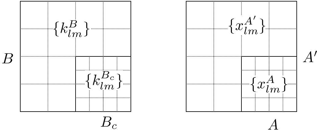
Figure 1: The construction of $\{f^{AB}_{lm}\}$ using $\{f^{A^{\prime}B_{c}}_{lm}\}$. $B_{c}$ is one of $B$’s child boxes and $A^{\prime}$ is $A$’s parent box. We first evaluate the potentials $\{u^{AB}_{lm}\}$ located at $\{x^{A}_{lm}\}$ using $f^{A^{\prime}B_{c}}_{l^{\prime}m^{\prime}}$ and then find $\{f^{AB}_{lm}\}$ so that they produce the same potentials.

The procedure we just described fails to be efficient when we compute $\{f^{AB}_{lm}\}$ for a large box $B$, as typically $B$ contains a large number of points $\{k_{j}\}$ and this makes the evaluation of $\{u^{AB}_{lm}\}$ quite expensive. The second ingredient of the butterfly algorithm addresses this problem. In our setting, suppose that $B$ is a non-leaf box of $T_{K}$, $A$ is a box in $T_{X}$, and $w^{A}w^{B}=N$. We denote the children of $B$ by $B_{c},c=1,\cdots,4$ and the parent of $A$ by $A^{\prime}$. Suppose that one constructs the equivalent charges in a bottom-up traversal of $T_{K}$. Hence, when one reaches $B$, the equivalent charges of $B_{c}$ have already been computed. The idea is then to use the equivalent charges $\{f^{A^{\prime}B_{c}}_{lm}\}$ of $B_{c}$ to compute the check potentials $\{u^{AB}_{lm}\}$ since $A\subset A^{\prime}$; i.e.,

$$u^{AB}_{lm}\approx\sum_{c=1}^{4}\left(\sum_{l^{\prime}m^{\prime}}e^{2\pi\imath x^{A}_{lm}\cdot k^{B_{c}}_{l^{\prime}m^{\prime}}/N}f^{A^{\prime}B_{c}}_{l^{\prime}m^{\prime}}\right)$$

for any $l,m$. The inner sum $\sum_{l^{\prime}m^{\prime}}e^{2\pi\imath x^{A}_{lm}\cdot k^{B_{c}}_{l^{\prime}m^{\prime}}/N}f^{A^{\prime}B_{c}}_{l^{\prime}m^{\prime}}$ for each fixed $i$ can be rewritten into a matrix form $Ef$. Using again the Kronecker product, we can decompose $E$ as $E_{1}\otimes E_{2}$ where

$$E_{1}=\left(e^{2\pi\imath\left(c_{1}^{A}+l\frac{w^{A}}{p-1}\right)\left(c_{1}^{B_{c}}+l^{\prime}\frac{w^{B_{c}}}{p-1}\right)/N}\right)_{ll^{\prime}}\quad E_{2}=\left(e^{2\pi\imath\left(c_{2}^{A}+m\frac{w^{A}}{p-1}\right)\left(c_{2}^{B_{c}}+m^{\prime}\frac{w^{B_{c}}}{p-1}\right)/N}\right)_{mm^{\prime}}.$$

Expanding the formula for $E_{1}$, we get

$$(E_{1})_{ll^{\prime}}=e^{2\pi\imath\left(c^{A}_{1}+l\frac{w^{A}}{p-1}\right)c^{B_{c}}_{1}/N}\cdot e^{2\pi\imath\frac{ll^{\prime}}{(p-1)^{2}}\frac{w^{A}w^{B_{c}}}{N}}\cdot e^{2\pi\imath c^{A}_{1}\left(l^{\prime}\frac{w^{B_{c}}}{p-1}\right)/N}$$ (4)

Noticing that the first and the third terms depend only on $l$ and $l^{\prime}$ respectively and $w^{A}w^{B_{i}}/N=1/2$, we can write $E_{1}$ into a factorization $E_{1}=E_{11}\cdot H\cdot E_{12}$ where $E_{11}$ and $E_{12}$ are again diagonal matrices and the matrix $H$ given by $(H)_{ll^{\prime}}=e^{\pi\imath\frac{ll^{\prime}}{(p-1)^{2}}}$ is independent of $N$.

2.2 Algorithm

We now give the overall structure of our algorithm. It contains the following steps:

1. Construct the quadtrees $T_{X}$ and $T_{K}$ for the point sets $\{x_{i},i\in I\}$ and $\{k_{j},j\in J\}$, respectively. These trees are constructed adaptively and all the leaf boxes are of unit size.

2. Construct the equivalent charges for the leaf boxes in $T_{K}$. Suppose that $A_{0}$ is the root box of $T_{X}$. For each leaf box $B$ in $T_{K}$, we calculate $\{f^{A_{0}B}_{lm}\}$ by matching the potentials $\{u^{A_{0}B}_{lm}\}$.

3. Travel up in $T_{K}$ and construct the equivalent charges for the non-leaf boxes in $T_{K}$. For each non-leaf box $B$ in $T_{K}$ and each box $A$ in $T_{X}$ with width $w^{A}=N/w^{B}$, we construct $\{f^{AB}_{lm}\}$ from the equivalent charges of $\{f^{A^{\prime}B_{c}}_{lm}\}$ where $A^{\prime}$ is $A$’s parent and $\{B_{c},c=1,\cdots,4\}$ are the $B$’s children.

4. Compute $\{u_{j},j\in J\}$. Let $B_{0}$ be the root box of $T_{K}$. For each leaf box $A$ in $T_{X}$ and each $j$ such that $x_{j}\in A$, we approximate $u_{j}$ with

   $$\sum_{lm}e^{2\pi\imath x_{j}\cdot k^{B_{0}}_{lm}/N}f^{AB_{0}}_{lm}.$$

Let us first estimate the number of operations of the proposed algorithm. The first step clearly takes only $O(N\log N)$ operations since there are at most $O(N)$ points in both $\{x_{i},i\in I\}$ and $\{k_{j},j\in J\}$. By assumption, both $X$ and $K$ are smooth (or piecewise smooth) curves in $[0,1]^{2}$. Therefore, for a given size $w$, there are at most $O(N/w)$ non-empty boxes in both $T_{X}$ and $T_{K}$. In particular, we have at most $O(N)$ leaf boxes in $T_{X}$ and $T_{K}$. This implies that the second and fourth steps take at most $O(N)$ operations. To analyze the third step, we estimate level by level. For a fixed level $t$, there are at most $2^{t}$ non-empty boxes in $T_{K}$ on that level, each of size $N/2^{t}$. For each box $B$ on level $t$, we need to construct $\{f^{AB}_{lm}\}$ for all the boxes $A$ in $T_{X}$ with size $N/(N/2^{t})=2^{t}$. It is clear that there are at most $N/2^{t}$ non-empty boxes in $T_{X}$ of that size. Since the construction for each set of equivalent charges take only constant operations, the total complexity for level $t$ is $O(2^{t}\times N/2^{t})=O(N)$. As there are at most $O(\log N)$ levels, the third step takes at most $O(N\log N)$ operations. Summing over all the steps, we conclude that our algorithm is $O(N\log N)$.

Our algorithm is also efficient in terms of storage space. Since we give explicit construct formulas (3) and (4) for constructing the equivalent charges, we only need to store the equivalent charges during the computation. This is where our algorithm differs from the one in [13] where they need to require $O(N\log N)$ small matrices for the interpolative decomposition [7, 11]. As we mentioned early, at each level, we need to keep $O(N)$ equivalent charges, each of which takes $O(1)$ storage space. Noticing that, at any point of the algorithm, we only need to keep the equivalent charges for two adjacent levels, therefore the storage requirement of our algorithm is only $O(N)$.

The three dimensional case is similar. Since $X$ and $K$ are smooth surfaces in $[0,1]^{3}$, the number of points in $\{x_{i},i\in I\}$ and $\{k_{j},j\in J\}$ are $O(N^{2})$ instead. The Kronecker product decomposition is still valid and, therefore, we can construct the equivalent charges efficiently in $O(p^{4})$ (or even $O(p^{3}\log p)$) operations instead of $O(p^{6})$. The algorithm remains exactly the same and a similar complexity analysis gives an operation count of $O(N^{2}\log N)$, which is almost linear in terms of the number of points.

3 Numerical Results

In this section, we provide some numerical examples to illustrate the properties of our algorithm. All of the numerical results are obtained on a desktop computer with a 2.8GHz CPU. The accuracy of the algorithm depends on $p$, which is the size of the Cartesian grid used for the equivalent charges. In the following examples, we pick $p=5,7$, or $9$. The larger the value of $p$, the better the accuracy.

3.1 2D case

For each example, we sample the curves $NX$ and $NK$ with 5 points per unit length. $\{f_{j},j\in J\}$ are randomly generated numbers with mean $0$. Suppose we use $\{u^{a}_{i},i\in I\}$ to denote the results of our algorithm. To study the accuracy of our algorithm, we pick a set $S\subset I$ of size 200 and estimate the error by

$$\sqrt{\frac{\sum_{i\in S}|u_{i}-u_{i}^{a}|^{2}}{\sum_{i\in S}|u_{i}|^{2}}}$$

where $\{u_{i},i\in S\}$ are the exact potentials computed by direct evaluation.

Before reporting the numerical results, let us summarize the notations that are used in the tables. $N$ is the size of the domain, $p$ is the size of the Cartesian grid used for the equivalent charges, $P$ is the maximum of the numbers of points in $\{x_{i}\}$ and $\{k_{j}\}$, $T_{a}$ is the running time of our algorithm in seconds, $T_{d}$ is the estimated running time of the direct evaluation in seconds, $T_{d}/T_{a}$ is the speedup factor, and finally $\varepsilon_{a}$ is the approximation error.

$(N,p)$	$P$	$T_{a}$(sec)	$T_{d}$(sec)	$T_{d}/T_{a}$	$\varepsilon_{a}$
(1024,5)	1.64e+4	1.23e+0	3.52e+1	2.86e+1	1.66e-3
(2048,5)	3.28e+4	2.71e+0	1.46e+2	5.38e+1	1.76e-3
(4096,5)	6.55e+4	6.05e+0	5.77e+2	9.53e+1	1.94e-3
(8192,5)	1.31e+5	1.32e+1	2.35e+3	1.78e+2	1.97e-3
(16384,5)	2.62e+5	2.89e+1	9.40e+3	3.25e+2	2.00e-3
(32768,5)	5.24e+5	6.27e+1	3.76e+4	5.99e+2	2.11e-3
(1024,7)	1.64e+4	2.07e+0	3.60e+1	1.74e+1	9.31e-6
(2048,7)	3.28e+4	4.64e+0	1.44e+2	3.11e+1	9.20e-6
(4096,7)	6.55e+4	1.03e+1	5.83e+2	5.68e+1	1.03e-5
(8192,7)	1.31e+5	2.27e+1	2.35e+3	1.04e+2	1.04e-5
(16384,7)	2.62e+5	5.14e+1	9.40e+3	1.83e+2	1.07e-5
(32768,7)	5.24e+5	1.18e+2	3.76e+4	3.18e+2	1.18e-5
(1024,9)	1.64e+4	3.31e+0	3.60e+1	1.09e+1	4.77e-8
(2048,9)	3.28e+4	7.23e+0	1.44e+2	1.99e+1	5.85e-8
(4096,9)	6.55e+4	1.59e+1	5.80e+2	3.65e+1	5.05e-8
(8192,9)	1.31e+5	3.57e+1	2.35e+3	6.59e+1	5.75e-8
(16384,9)	2.62e+5	7.74e+1	9.40e+3	1.21e+2	6.16e-8
(32768,9)	5.24e+5	1.87e+2	3.76e+4	2.01e+2	5.94e-8

Table 1: 2D results. Top: Both $X$ and $K$ are ellipses in unit box $[0,1]^{2}$. Bottom: Running time, speedup factor and accuracy for different combinations of $N$ and $p$. $N$ is the size of the domain, $p$ is the size of the Cartesian grid used for the equivalent charges, $P$ is the maximum of the numbers of points in $\{x_{i}\}$ and $\{k_{j}\}$, $T_{a}$ is the running time of our algorithm in seconds, $T_{d}$ is the estimated running time of the direct evaluation in seconds, $T_{d}/T_{a}$ is the speedup factor, and finally $\varepsilon_{a}$ is the approximation error.

$(N,p)$	$P$	$T_{a}$(sec)	$T_{d}$(sec)	$T_{d}/T_{a}$	$\varepsilon_{a}$
(1024,5)	1.64e+4	1.93e+0	3.60e+1	1.87e+1	1.52e-3
(2048,5)	3.28e+4	4.25e+0	1.46e+2	3.43e+1	1.67e-3
(4096,5)	6.55e+4	9.49e+0	5.80e+2	6.11e+1	1.66e-3
(8192,5)	1.31e+5	2.06e+1	2.34e+3	1.14e+2	1.69e-3
(16384,5)	2.62e+5	4.59e+1	9.50e+3	2.07e+2	1.99e-3
(32768,5)	5.24e+5	9.85e+1	3.78e+4	3.84e+2	1.84e-3
(1024,7)	1.64e+4	3.20e+0	3.60e+1	1.13e+1	7.81e-6
(2048,7)	3.28e+4	7.12e+0	1.44e+2	2.02e+1	8.26e-6
(4096,7)	6.55e+4	1.60e+1	5.77e+2	3.60e+1	8.79e-6
(8192,7)	1.31e+5	3.54e+1	2.34e+3	6.61e+1	9.25e-6
(16384,7)	2.62e+5	8.14e+1	9.52e+3	1.17e+2	9.07e-6
(32768,7)	5.24e+5	1.91e+2	3.76e+4	1.97e+2	1.07e-5
(1024,9)	1.64e+4	5.02e+0	3.52e+1	7.02e+0	4.24e-8
(2048,9)	3.28e+4	1.12e+1	1.43e+2	1.28e+1	4.77e-8
(4096,9)	6.55e+4	2.47e+1	5.87e+2	2.37e+1	4.65e-8
(8192,9)	1.31e+5	5.60e+1	2.33e+3	4.17e+1	4.35e-8
(16384,9)	2.62e+5	1.24e+2	9.40e+3	7.60e+1	4.99e-8
(32768,9)	5.24e+5	2.84e+2	3.76e+4	1.32e+2	6.04e-8

Table 2: 2D results. Top: $X$ and $K$ are two smooth curves in unit box $[0,1]^{2}$. Bottom: Running time, speedup factor and accuracy for different combinations of $N$ and $p$.

Tables 1 and 2 report the results for two testing examples. From these tables, it is quite clear that the complexity of our algorithm grows indeed almost linearly in terms of the number of points, and its accuracy is stably controlled by the value of $p$. For larger values of $N$, we obtain a substantial speedup over the direct evaluation.

3.2 3D case

We apply our algorithm to the problem of computing the far field pattern (2). In this setup, $X$ is always a sphere, while $K$ is the boundary of the scatter. We sample the surface $NX$ and $NK$ again with about $5\times 5=25$ points per unit area. Tables 3 and 4 summarize the results of two typical examples in evaluating the far field pattern of scattering fields.

$(N,p)$	$P$	$T_{a}$(sec)	$T_{d}$(sec)	$T_{d}/T_{a}$	$\varepsilon_{a}$
(16,5)	2.14e+4	2.49e+0	1.50e+1	6.03e+0	1.24e-3
(32,5)	8.19e+4	9.78e+0	1.88e+2	1.93e+1	1.52e-3
(64,5)	3.22e+5	3.94e+1	2.77e+3	7.03e+1	1.44e-3
(128,5)	1.28e+6	1.62e+2	4.39e+4	2.71e+2	1.68e-3
(256,5)	5.13e+6	6.77e+2	7.00e+5	1.03e+3	1.79e-3
(16,7)	2.14e+4	6.77e+0	1.50e+1	2.22e+0	5.80e-5
(32,7)	8.19e+4	2.66e+1	1.80e+2	6.79e+0	7.24e-5
(64,7)	3.22e+5	1.07e+2	2.74e+3	2.55e+1	7.98e-5
(128,7)	1.28e+6	4.40e+2	4.39e+4	9.98e+1	7.89e-5
(16,9)	2.14e+4	1.43e+1	1.50e+1	1.05e+0	2.40e-7
(32,9)	8.19e+4	5.64e+1	1.88e+2	3.34e+0	3.25e-7
(64,9)	3.22e+5	2.28e+2	2.74e+3	1.20e+1	3.24e-7
(128,9)	1.28e+6	9.38e+2	4.44e+4	4.74e+1	3.33e-7

Table 3: 3D results. Top: the surface $K$ is the boundary of an F16 airplane model. Bottom: Running time, speedup factor and accuracy for different combinations of $N$ and $p$.

$(N,p)$	$P$	$T_{a}$(sec)	$T_{d}$(sec)	$T_{d}/T_{a}$	$\varepsilon_{a}$
(16,5)	2.14e+4	3.20e+0	1.07e+1	3.35e+0	1.45e-3
(32,5)	8.19e+4	1.25e+1	1.39e+2	1.12e+1	1.65e-3
(64,5)	3.22e+5	5.11e+1	2.13e+3	4.17e+1	1.79e-3
(128,5)	1.28e+6	2.02e+2	3.46e+4	1.71e+2	2.19e-3
(256,5)	5.13e+6	8.31e+2	5.54e+5	6.67e+2	1.94e-3
(16,7)	2.14e+4	8.72e+0	1.07e+1	1.23e+0	7.06e-5
(32,7)	8.19e+4	3.39e+1	1.39e+2	4.11e+0	7.57e-5
(64,7)	3.22e+5	1.35e+2	2.13e+3	1.57e+1	9.05e-5
(128,7)	1.28e+6	5.48e+2	3.44e+4	6.28e+1	1.04e-4
(16,9)	2.14e+4	1.85e+1	8.58e+0	4.64e-1	2.61e-7
(32,9)	8.19e+4	7.19e+1	1.39e+2	1.94e+0	3.00e-7
(64,9)	3.22e+5	2.87e+2	2.13e+3	7.41e+0	4.38e-7
(128,9)	1.28e+6	1.17e+3	3.52e+4	3.01e+1	3.46e-7

Table 4: 3D results. Top: the surface $K$ is the boundary of a submarine model. Bottom: Running time, speedup factor and accuracy for different combinations of $N$ and $p$.

4 Conclusions and Discussions

In this paper, we introduced an efficient algorithm for computing sparse Fourier transforms located on curves and surfaces. Our algorithm, which is an extension of the butterfly algorithm, is accurate and has provably $O(N\log N)$ complexity. The success of the algorithm is based on an low rank property concerning the interaction between spatial and frequency regions that follow a certain geometrical condition. We use equivalent sources supported on Cartesian grids as the low rank representation and exploit the tensor-product property of the Fourier transform to achieve maximum efficiency. Furthermore, our algorithm requires only linear storage space.

The problem considered in this paper is only one example of many computational issues regarding highly oscillatory behaviors. Some other examples include the computation of Fourier integer operators [14], scattering fields for high frequency waves [8], and Kirchhoff migrations [3]. In the past two decades, many algorithms have been developed to address these challenging computational tasks efficiently. Some examples include [4, 6, 1, 5, 9]. It would be interesting to see whether the ideas behind these approaches can be used to study the problem addressed in this paper, and vice versa.

Acknowledgments. The research presented in this paper was supported by an Alfred P. Sloan Fellowship and a startup grant from the University of Texas at Austin.

References

- [1] A. Averbuch, E. Braverman, R. Coifman, M. Israeli, and A. Sidi. Efficient computation of oscillatory integrals via adaptive multiscale local Fourier bases. Appl. Comput. Harmon. Anal., 9(1):19–53, 2000.
- [2] D. H. Bailey and P. N. Swarztrauber. The fractional Fourier transform and applications. SIAM Rev., 33(3):389–404, 1991.
- [3] G. Beylkin. The inversion problem and applications of the generalized Radon transform. Comm. Pure Appl. Math., 37(5):579–599, 1984.
- [4] O. P. Bruno and L. A. Kunyansky. A fast, high-order algorithm for the solution of surface scattering problems: basic implementation, tests, and applications. J. Comput. Phys., 169(1):80–110, 2001.
- [5] E. Candès, L. Demanet, and L. Ying. Fast computation of fourier integral operators. SIAM Journal on Scientific Computing, 29(6):2464–2493, 2007.
- [6] H. Cheng, W. Y. Crutchfield, Z. Gimbutas, L. F. Greengard, J. F. Ethridge, J. Huang, V. Rokhlin, N. Yarvin, and J. Zhao. A wideband fast multipole method for the Helmholtz equation in three dimensions. J. Comput. Phys., 216(1):300–325, 2006.
- [7] H. Cheng, Z. Gimbutas, P. G. Martinsson, and V. Rokhlin. On the compression of low rank matrices. SIAM J. Sci. Comput., 26(4):1389–1404 (electronic), 2005.
- [8] D. L. Colton and R. Kress. Integral equation methods in scattering theory. Pure and Applied Mathematics (New York). John Wiley & Sons Inc., New York, 1983.
- [9] B. Engquist and L. Ying. Fast directional multilevel algorithms for oscillatory kernels. SIAM Journal on Scientific Computing, 29(4):1710–1737, 2007.
- [10] S. Fomel and L. Ying. Fast computation of partial Fourier transforms. Technical report, University of Texas at Austin, 2007.
- [11] M. Gu and S. C. Eisenstat. Efficient algorithms for computing a strong rank-revealing QR factorization. SIAM J. Sci. Comput., 17(4):848–869, 1996.
- [12] E. Michielssen and A. Boag. A multilevel matrix decomposition algorithm for analyzing scattering from large structures. IEEE Transactions on Antennas and Propagation, 44(8):1086–1093, 1996.
- [13] M. O’Neil and V. Rokhlin. A new class of analysis-based fast transforms. Technical report, Yale University. YALE/DCS/TR1384, 2007.
- [14] E. M. Stein. Harmonic analysis: real-variable methods, orthogonality, and oscillatory integrals, volume 43 of Princeton Mathematical Series. Princeton University Press, Princeton, NJ, 1993. With the assistance of Timothy S. Murphy, Monographs in Harmonic Analysis, III.