A Multifractal Analysis of Asian Foreign Exchange Markets
Abstract
We analyze the multifractal spectra of daily foreign exchange rates for Japan, Hong-Kong, Korea, and Thailand with respect to the United States Dollar from 1991 to 2005. We find that the return time series show multifractal spectrum features for all four cases. To observe the effect of the Asian currency crisis, we also estimate the multifractal spectra of limited series before and after the crisis. We find that the Korean and Thai foreign exchange markets experienced a significant increase in multifractality compared to Hong-Kong and Japan. We also show that the multifractality is stronge related to the presence of high values of returns in the series.
pacs:
89.65.-s, 89.65.Gh, 89.20.-aI Introduction
Economic systems are widely acknowledged as extremely complex, and have recently become an interesting area of study for physicists as well as economists Mantegna&Bouchaud . Many previous studies have found that time series of financial markets exhibit some non-linear properties developed in statistical physics Mantegna(a) ; Oh . The prices in financial markets are created by non-trivial interactions among heterogeneity agents and complex events occurring in the external environment. In other words, both micro and macro variables with various time scales are involved in the pricing mechanism.
The properties observed in financial time series include long-memory in volatility Oh , a multifractal nature Muzy ; Sornette ; Plamen ; Parisi ; Mandelbrot , and fat tails Mantegna(a) among others; these are sometimes referred to as the stylized facts. The multifractal concept, which is now well developed in the fields of statistical physics and nonlinear dynamics, is a well-known feature of complex systems Plamen ; Parisi ; Mandelbrot ; Matia ; Kwapie . Multifractality has been discovered in systems as diverse as earthquakes Parisi , turbulence systems, biological time series Plamen , as well as financial markets Muzy ; Kwapie .
Previous studies have found evidence for a relationship between the complexity of a system and its degree of multifractality Plamen . For example, the degree of multifractality in data generated by a multiplicative cascading process is directly related to the long-range correlations of the magnitude time series Ashkenazy . Other factors that could affect the multifractality of time series include time correlations and the probability distribution of the data Matia ; Kwapie . However, it is still not clear what is the origin of multifractality in financial markets.
In this paper we study the multifractal properties of a financial time series: the daily return of four foreign exchange (FX) markets. We consider Japan (JPY/USD), Hong-Kong (HKD/USD), Korea (KRW/USD), and Thailand (THD/USD) from 1991 to 2005. We employ multifractal detrended fluctuation analysis (MF-DFA) Kantelhardt to measure the nonlinear features of the time series, in particular their multifractal spectra. To test their significance we randomly shuffle the series to remove any temporal correlations, and find that these spectra narrow significantly. In other words, we find that temporal correlation plays an important rule in the multifractality of the data, similar to Matia et al. Matia .
To detect changes in market complexity before and after the Asian currency crisis, we divide the series into two periods before and after the crash and calculate their multifractal spectra separately. We find that for Korean and Thailand the degree of multifractality increased significantly after the Asian currency crisis, while the FX markets of Hong Kong and Japan did not. We therefore suggest that both Korea and Thailand have been more influenced by the Asian currency crisis. We also examine the effect of return values above a certain threshold in the FX markets on the market complexity. We find that for all countries, market complexity is related to higher returns.
In the next Section, we describe the financial data and our methodology. In Section 3, we present our results of this study. Section 4 concludes the article.
II Data and Methodology
We investigate the multifractal properties of Asian FX markets (returns to U.S. Dollars) from 1991 to 2005 for four countries: Japan (JPY/USD), Hong-Kong (HKD/USD), Korea (KRW/USD), and Thailand (THB/USD). The data are obtained from http://www.federal/reserve.gov/RELEASES/. In all data sets used in this paper, we remove the year 1997 to eliminate any abnormalities due to the market crash itself. The return time series is calculated by the log-difference of daily prices: , where is the foreign exchange rate on day . We divide the whole series into two sub-periods: DATA A from 1991 to 1996 (before the crisis) and DATA B from 1998 to 2005 (after the crisis). This allows us to study the influence of the Asian currency crisis on market complexity. We employ the multifractal detrended fluctuation analysis (MF-DFA) method to determine the multifractal properties of the time series. The MF-DFA method was proposed by Kantelhardt et al. Kantelhardt , and can be explained by the following three steps.
Step (1): We subtract the average value of the time series from each point , then accumulate the series:
| (1) |
where is the point and is the mean of all . This step represents the original data as an accumulated profile, .
Step (2): The profile is divided into boxes of length . In each box , the trend is estimated by an -order polynomial using the least-squares method. The best-fit curve of a given box is expressed as . By subtracting from , possible trends are removed Peng . This process is applied to every box, and the fluctuations in that box are then calculated as
| (2) |
Step (3): We compute the mean -order moment of the series by averaging the appropriate function of over all boxes. In this way we obtain a scaling relation with box size :
| (3) |
The exponent depends on . In general, the multifractal (MF) scaling exponent is related to through
| (4) |
where is the fractal dimension of a geometric object. In our case, . The MF exponent represents the temporal structure of the time series as a function of the various moments . That is, reflects the scale-dependence of smaller fluctuations for negative values of , and larger fluctuations for positive values of . In the special case that is a linear function, the time series can be regarded as a monofractal and is the singularity strength or Hölder exponent. If increases nonlinear with , then the series is multifractal. In this case we can calculate the MF spectrum by a Legendre transform of , as defined by
| (5) |
where is the dimension of the time series. If the time series is monofractal, is a delta function, there is only one value of ; otherwise, there is a distribution of values.
III Results
We have analyzed the multifractal spectra of Asian FX markets using the above MF-DFA method. The pricing mechanisms may well be complex, due to the Asian currency crisis in late 1997 as well as due to various internal and external events. The Asian currency crisis had an impact on almost all Asian FX markets Gabjin . Here, we study the multifractal properties of four markets and try to identify how the crisis may have affected their multifractality.
In Fig. 1, we show the return time series of Hong-Kong (a), Japan (b), Korea (c), and Thailand (d). The Korean and Thai FX markets clearly have higher volatility after the Asian currency crisis in 1997, but the Japanese and Hong-Kong markets show no obvious change.
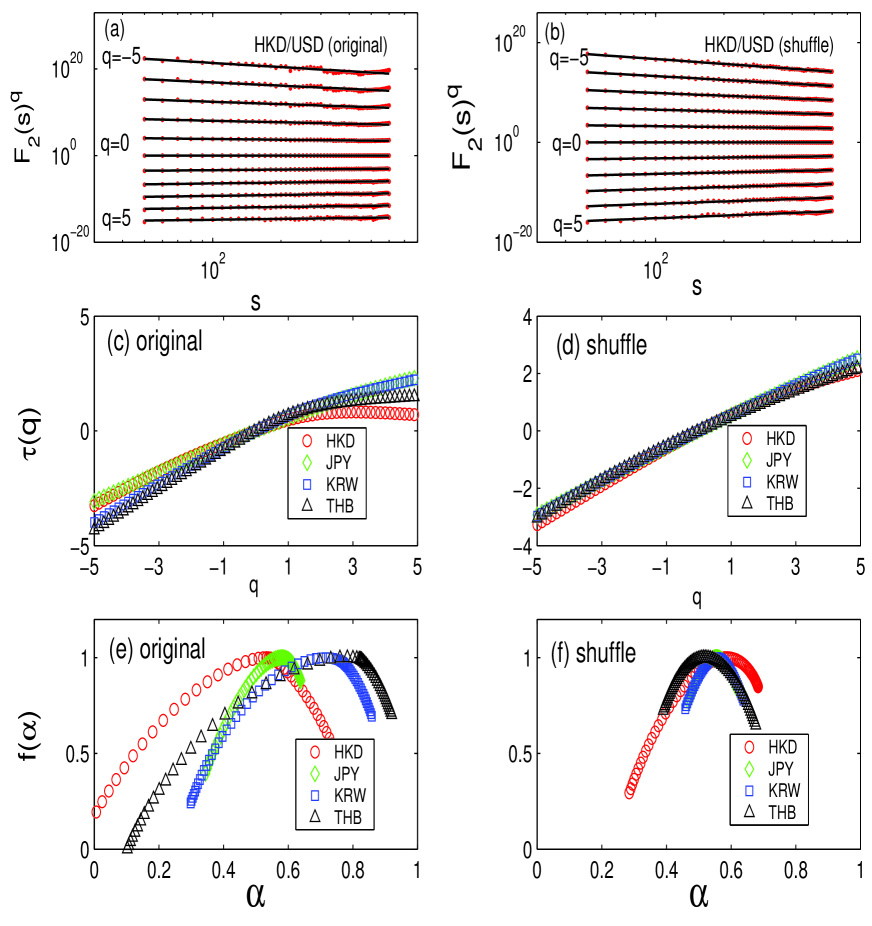
We now describe the multifractal properties of the four markets. The results of MF-DFA analysis are presented in Fig. 2. To test how significant is the multifractality, we also perform the analysis on shuffled time series created by randomly shuffling the data. Figs. 2(a) and (b) show the fluctuation spectra of the original and shuffled HKD/USD series respectively. These logarithmic plots indicate that in both cases is a power-law with an exponents depending on . Fig. 2(c) and (d) display the multifractal scaling function of the original and shuffled data. We calculated from the power-law relation between and , using scales in the range . This is since below there is discreteness effects (original and shuffled). We find that the two datasets behave similarly almost linear with q for negative moments, but show significant non-linearities for positive moments. This means that the larger fluctuations have changed dramatically in the shuffled series.
To explicitly observe the multifractality we can convert and to and by a Legendre transform. Fig. 2(e) shows the multifractal spectra of the original market series. We find that the singularity strengths of the markets lie within the following ranges: , , , and . Fig. 2(f) presents the same information for the shuffled time series: , , , and . Figs. 2(e) and (f) show that the multifractal spectra are narrower for the surrogate time series, from which all temporal correlations have been removed. Our results indicate that the temporal fluctuations in Asian FX markets show signature of multifractality.
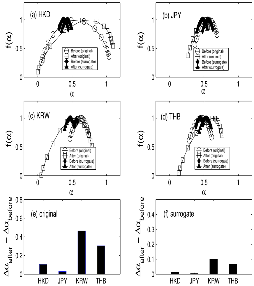
The Asian currency crisis had an influence on almost all the Asian FX markets, so it is reasonable to assume that their status may have changed significantly. An interesting question is how the Asian currency crisis has influenced the market complexity. We divided each time series into two sub-periods: (DATA A) and (DATA B) before and after the crisis respectively. Fig. 3 shows the multifractal spectra of the original and surrogate time series, which remove the nonlinearity from the original data Theiler , of both periods for all four FX markets. We find that the multifractal spectra of all the surrogate data set is reduced significantly than those of the original data. The Hong Kong and Japanese FX markets show a similar degree of multifractality before and after the crisis, while the Korean and Thai markets change significantly and the multifractal spectra become broader. In other words, the complexity of the Korean and Thai FX markets has been increased after the Asian currency crisis. Fig. 3(e) and (f) shows the change in the degree of multifractality of both the original and surrogate data for each market. We conjecture that since the Japanese FX market is the most mature, it was also the least influenced by the Asian currency crisis. The emerging markets of Korea and Thailand, on the other hand, were greatly influenced by the crash. As for the Hong Kong FX market, since Hong Kong chose to have a fixed exchange rate with the U.S. dollar (called the Peg system) both periods have similar broad spectra. The Asian currency crisis thus increased the complexity of the Korean and Thai FX markets, perhaps because its aftermath spurred the development of new government policies in those countries.
Table 1 shows the degree of multifractality of the original, shuffled data and before and after the crisis for all countries used in this paper. This quantity shows that for the original data the multifractal spectra have more broader than those of shuffled data and the degree of multifractality both the Korean and Thailand FX markets increases significantly after the crisis.
We have observed that temporal correlations are not linear but posses multifractality in the time series. It is interesting to note that the shuffled time series removed the time correlation still show some multifractality. It is widely accepted that the distribution of returns in a financial market follows a power law, with an exponent close to 3 Mantegna(a) . In other words, there are many higher values that cannot be predicted by the pricing mechanism of the efficiency market hypothesis (EMH) Fama , which is also widely used in the financial literature. We will now investigate the influence of high returns on the multifractality. To do this, we generate a multifractal noise data set using the wavelet-cascade model introduced by Arneodo et. al. Arneodo . We employ the log-normal random variable to generate the multifractal noise data. In this case, the degree of multifractality of the created data is determined by the parameters such as the mean, , and the standard deviation, , of and it is positively related to the value. Where is a coefficient of the normal distribution with and . We can create the artificial data that have the different degree of multifractality with respective to the mean, , and the standard deviation, . The multifractal spectrum is given by and the multifractal spectrum width as the degree of multifractality is .
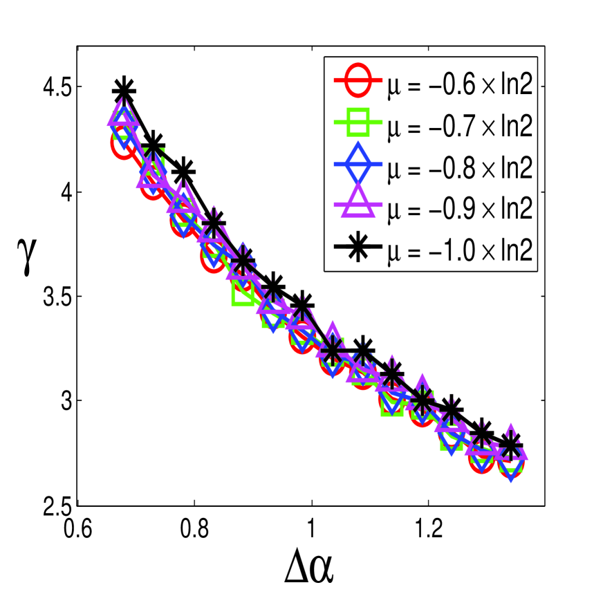
To verify the relationship between the degree of multifractality and the extreme values, we creates 100 data sets with data points and calculate the tail exponent, , of power law distribution, using method proposed by A. Clauset et. al. Clauset . Fig. 4 shows the relationship between the degree of multifractality and the power-law exponents using the multifractal noise data sets created with and various values in the ranges from 0.2 to 0.4. The circles (red), sqaures (green), diamons (blue), triangles (pink), and stars(black) correspond to the multifractal noise data created with , }, respectively. In Fig. 4, we observe that regardless of , the exponent, increases as the degree of multifractality increases. In other words, the degree of multifractality has strongly relation to the existing of the extreme values in the multifractal noise data.
To verify the result observed in the Fig. 4 to the foreign exchange markets, we create a new version of each time series by eliminating values above a certain threshold, in units of the standard deviation of the time series. The eliminated data points are replaced by linear interpolation. As the threshold increases, the time series will retain higher values.
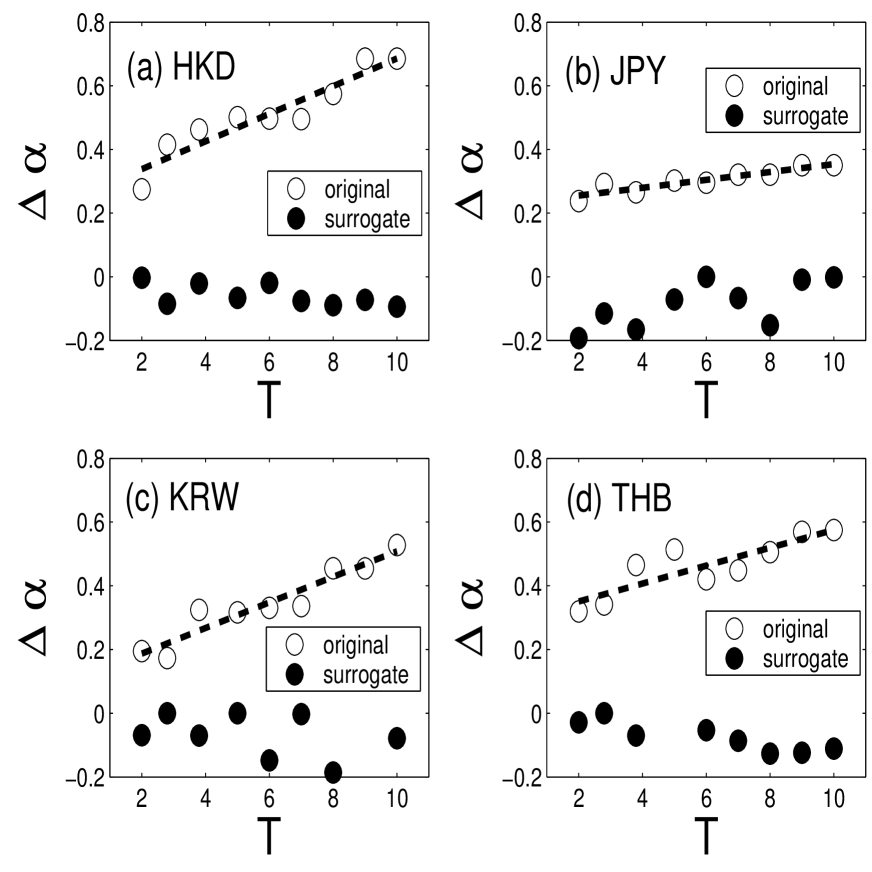
Fig. 5(a), (b), (c), and (d) display the dependence of the degree of multifractality , defined by the range of singularity strengths , on the threshold for original and surrogate data. The open and filled circles indicate the original and surrogate data, respectively. We find that in all four countries, FX market complexity is related to the presence of very high return values. However, for the surrogate data removed the nonlinearity from the original data is an independent from the threshold T. Market values are created by non-trivial interactions between heterogeneity agents and the influence of internal and external events. The results of Fig. 5 seem to indicate that more complex markets are more likely to produce high returns.
IV Conclusions
We investigated the properties of time series from four Asian foreign exchange markets, and found two factors affecting their multifractality as measured by the MF-DFA method. First, we found that temporal correlations in the data contribute to the multifractality of all four FX markets. Second, we find that market complexity and multifractality are positively related to the presence of high return values in the series. Further studies will examine both aspects of FX markets more extensively.
To observe how the Asian currency crisis influenced these FX markets, we estimated their multifractal properties both before and after the crisis. We found that in both Korea and Thailand, the degree of multifractality in the FX market significantly increased after the Asian currency crisis. Japan and Hong Kong, however, were almost unaffected. We argue that the market crash affected Korea and Thailand more strongly because they are typical emerging markets; these countries probably introduced new policies (and thus additional complexities) to help control the aftermath. Japan’s mature market was little changed by the crisis, however, and Hong Kong uses a fixed exchange rate.
Acknowledgements.
This work was supported partially by the Korea Research Foundation Grant funded by the Korean Government (KRF-2007-412-J02303) and partially by the KOSEF under the grant number R01-2008-000-21065-0.References
- (1) R. N. Mantegna and H. E. Stanley, An Introduction to Econophysics: Correlation and Complexity in Finance (Cambridge University Press, Cambridge, U.K., 1999); J-P. Bouchaud, M. Potters Theory of Financial Risk and Derivative Pricing: From Statistical Physics to Risk Management (Cambridge University Press, Cambridge, USA, 2004);
- (2) R. N. Mantegna et al., Nature, 376 46 (1995); R. N. Mantegna et al., Nature, 383 587 (1996); V. Plerou et al., Nature, 421 130 (2003); X. Gabaix et al., Nature, 423 267 (2003);
- (3) Y. Liu et al., Phys. Rev. E, 60 1390 (1999); K. Yamasaki et al., Proc. Natl. Acad. Sci., 102 9424 (2005); G. Oh et al., J. Korean Phys. Soc., 48 197 (2006); F. Wang et al., Phys. rev. E, 73 066128 (2006);
- (4) J. F. Muzy et al., Eur. Phys. J. B, 17 537 (2000); Z. Eisler et al., Physica A, 343 603 (2004); L. Calvet et al., J. of Econometrics, 105 27 (2001);
- (5) D. Sornette and G. Ouillon, Phys. Rev. E, 94 038501 (2005);
- (6) P. Ch. Ivanov, L. A. N. Amaral, A. L. Goldberger, S. Havlin, M. G. Rosenblum, Z. Struzik, and H. E. Stanley, Nature, 399 461 (1999);
- (7) G. Parisi and U. Frisch, in Turbulence and Predictability in Geophysical Fluid Dynamics and Climate Dynamics, Proceedings of the International School ”Enrico fermi,” (North-Holland, Amsterdam, 1985);
- (8) B. B. Mandelbrot, Fractals and Scaling In Finance (Springer, 1997);
- (9) Y. Ashkenazy, S. Havlin, P. Ch. Ivanov, C.-K. Peng, V. Schulte-Frohlinde, and H. E. Stanley, Physica A, 323 19 (2003);
- (10) C.K. Peng, S.V. Buldyrev, A.L. Goldberger, S.Havlin, M. Simons, and H. E. Stanley, Phys. Rev. E 47, 3730 (1994)
- (11) K. Matia, Y. Ashkenazy, and H. E. Stanley, Europhys. Lett., 61 422 (2003);
- (12) J. Kwapień, P. O świecimka and S. Droźdź, Physica A, 350 466 (2005);
- (13) J. W. Kantelhardt, S. Zschiegner, E. Koscielny-Bunde, S. Havlin, A. Bunde, and H. E. Stanley, Physica A, 316 87 (2002);
- (14) G. Oh, S. Kim, and C. Eom, Physica A, 382 209 (2007);
- (15) J. Theiler, S. Eubank, A. Lontin, B. Galdrikian and J. Doyne, Physica D 58, 77 (1992).
- (16) E. F. Fama, Journal of Finance, 25 383 (1970);
- (17) A. Arneodo, E. Bacry, and J.F. Muzy, J. Math. Phys. 39, 4142 (1998);
- (18) A. Clauset, C.R. Shalizi, and M.E.J. Newman, arXiv:0706.1062v2 (2009)

| Country | Original () | Shuffled () | Before () | After () |
|---|---|---|---|---|
| HongKong | 1.14 | 0.55 | 0.98 | 1.09 |
| Japan | 0.29 | 0.15 | 0.32 | 0.34 |
| Korea | 0.55 | 0.20 | 0.27 | 0.73 |
| Thailand | 0.83 | 0.28 | 0.32 | 0.63 |