The Distribution of Stellar Mass in the Pleiades

Abstract

As part of an effort to understand the origin of open clusters, we present a statistical analysis of the currently observed Pleiades. Starting with a photometric catalog of the cluster, we employ a maximum likelihood technique to determine the mass distribution of its members, including single stars and both components of binary systems. We find that the overall binary fraction for unresolved pairs is 68%. Extrapolating to include resolved systems, this fraction climbs to about 76%, significantly higher than the accepted field-star result. Both figures are sensitive to the cluster age, for which we have used the currently favored value of 125 Myr. The primary and secondary masses within binaries are correlated, in the sense that their ratios are closer to unity than under the hypothesis of random pairing. We map out the spatial variation of the cluster’s projected and three-dimensional mass and number densities. Finally, we revisit the issue of mass segregation in the Pleiades. We find unambiguous evidence of segregation, and introduce a new method for quantifying it.

1 Introduction

Open clusters, with their dense central concentrations of stars, are relatively easy to identify. Over a thousand systems are known, and the census is thought to be complete out to 2 kpc (Brown, 2001; Dias et al., 2002). Because the clusters are no longer buried within interstellar gas and dust, their internal structure and dynamics is also more accessible than for younger groups.

Despite these favorable circumstances, many basic questions remain unanswered. Most fundamentally, how do open clusters form? All observed systems have undergone some degree of dynamical relaxation. Thus, the present-day distribution of stellar mass differs from the one just after disruption of the parent cloud. Recovering this initial configuration will clearly be of value in addressing the formation issue. But such reconstruction presupposes, and indeed requires, that we gauge accurately the stellar content of present-day clusters. Even this simpler issue is a non-trivial one, as we show here.

We consider one of the most intensively studied open clusters, the Pleiades. Again, our ultimate goal is to trace its evolution from the earliest, embedded phase to the present epoch. Focusing here on the latter, we ask the following questions: What are the actual masses of the member stars? Do they follow the field-star initial mass function? How many of the members are single, and how many are in binary pairs? Are the primary and secondary masses of binaries correlated? What is the overall density distribution in the cluster? What is the evidence for mass segregation, and how can this phenomenon be quantified?

All of these questions have been addressed previously by others. Deacon & Hambly (2004) constructed a global mass function for the Pleiades. Their method was to assign masses based on the observed distribution of $R$-magnitudes. A more accurate assessment should account for the photometric influence of binaries. Several studies directed specifically at binaries have probed selected regions for spectroscopic pairs (Raboud & Mermilliod, 1998; Bouvier et al., 1997). However, the overall binary fraction has not been carefully assessed, despite some preliminary attempts (Steele & Jameson, 1995; Bouvier et al., 1997; Moraux et al., 2003).

A fuller investigation of these and the other issues raised requires statistical methods; these should prove generally useful in characterizing stellar populations. Section 2 describes our approach, which employs a regularized maximum likelihood technique (e.g. Cowen, 1998). A similar method has been applied to other astronomical problems, including the reconstruction of cloud shapes (Tassis, 2007) and the investigation of binarity within globular clusters (Romani & Weinberg, 1991). Our study is the first to apply this versatile tool to young stellar groups. In doing so, we also relax many of the restrictive assumptions adopted by previous researchers. Section 3 presents our derived mass function for the Pleiades, along with our results for binarity. The density distribution, as well our quantification of mass segregation, are the topics of Section 4. Finally, Section 5 summarizes our findings, critically reexamines the binarity issue, and indicates the next steps in this continuing study.

2 Method of Solution

2.1 Stellar Mass Probability Function

The basic problem is how to assign stellar masses to all the point-like sources believed to be cluster members. In many cases, the source is actually a spatially unresolved binary pair. More rarely, it is a triple or higher-order system; for simplicity, we ignore this possibility. The available observational data consists of photometry in several wavebands. Given the inevitable, random error associated with each photometric measurement, it is not possible to identify a unique primary and secondary mass for each source. Instead we adopt a statistical approach that finds the relative probability for each source to contain specific combinations of primary and secondary masses.

We introduce a stellar mass probability density, to be denoted $\Phi(m_{p},m_{s})$. This two-dimensional function is defined so that $\Phi(m_{p},m_{s})\,\Delta m_{p}\,\Delta m_{s}$ is the probability that a binary system exists with primary mass (hereafter expressed in solar units) in the interval $m_{p}$ to $m_{p}+\Delta m_{p}$ and secondary mass from $m_{s}$ to $m_{s}+\Delta m_{s}$. Single stars are viewed here as binaries with $m_{s}=0$. We normalize the function over the full mass range:

$$\int_{m_{\rm min}}^{m_{\rm max}}\!dm_{p}\int_{0}^{m_{p}}\!dm_{s}\,\Phi(m_{p},m_{s})\,=\,1\,\,.$$ (1)

Note that we integrate the secondary mass $m_{s}$ only to $m_{p}$, its maximum value. Furthermore, we set the lower limit of $m_{s}$ to 0, in order to account for single stars. It is assumed that $\Phi\,=\,0$ for $0\,<\,m_{s}\,<m_{\rm min}$. Here, the global minimum mass $m_{\rm min}$ is taken to be 0.08, the brown dwarf limit. We consider $m_{\rm max}$ to be the highest mass still on the main sequence. The age of the Pleiades has been established from lithium dating as $1.25\times 10^{8}$ yr (Stauffer et al., 1998). This figure represents the main-sequence lifetime for a star of $4~{}M_{\odot}$ (Siess et al., 2000), which we adopt as $m_{\rm max}$.

We examine separately the handful of stars that are ostensibly more massive than $m_{\rm max}$, and hence on post-main-sequence tracks. For these 11 sources, we assigned approximate masses from the observed spectral types, and obtained data on their known unresolved binary companions; this information was taken from the Bright Star Catalogue (Hoffleit et al., 1991). These systems were then added by hand to our mass functions. Finally, we ignore the brown dwarf population, thought to comprise from 10 to 16% of the total system mass (Pinfield et al., 1998; Schwartz & Becklin, 2005).

The most direct method for evaluating $\Phi(m_{p},m_{s})$ would be to guess its values over a discrete grid of $m_{p}$- and $m_{s}$-values. Each $(m_{p},m_{s})$ pair makes a certain contribution to the received flux in various wavebands. Thus, any guessed $\Phi(m_{p},m_{s})$ yields a predicted distribution of fluxes, which will generally differ from that observed. One changes the guessed function until the observed flux distribution is most likely to be a statistical realization of the predicted one.

Unfortunately, this straightforward approach is impractical. The basic difficulty is the mass-sensitivity of stellar luminosities. For secondary masses $m_{s}$ only modestly less than $m_{p}$, the binary is indistinguishable photometrically from a single star having the primary mass. A $0.6\ M_{\odot}$ main-sequence star, for example, has a $K$-band flux of 10.81 mag at the 133 pc distance of the Pleiades (Soderblom et al., 2005). Pairing this star with a $0.2~{}M_{\odot}$ secondary (which is not yet on the main sequence) only changes the flux to 10.68 mag. In summary, the function $\Phi(m_{p},m_{s})$ evaluated in this way is unconstrained throughout much of the $m_{p}-m_{s}$ plane.

2.2 Correlation within Binaries

Since binaries of even modestly large primary to secondary mass ratio are difficult to recognize observationally, we need to infer their contribution indirectly, within the context of a larger theoretical framework. The physical origin of binaries is far from settled (Zinnecker & Mathieu, 2001). There is a growing consensus, however, that most pairs form together, perhaps within a single dense core. The accumulating observations of protobinaries, i.e., tight pairs of Class 0 or Class I infrared sources, have bolstered this view (e.g., Haisch et al., 2004).

If binaries indeed form simultaneously, but independently, within a single dense core, there is no reason to expect a strong correlation between the component masses. (Such a correlation would be expected if the secondaries formed within the primaries’ circumstellar disks, for example.) A credible starting hypothesis, then, is that each component mass is selected randomly from its own probability distribution. If the formation mechanism of each star is identical, then these distributions are also the same. That is, we postulate that the true binary contribution to $\Phi(m_{p},m_{s})$ is $\phi(m_{p})\,\phi(m_{s})$, where the single-star probability density $\phi$ is properly normalized:

$$\int_{m_{\rm min}}^{m_{\rm max}}\!\phi(m)\,dm\,=\,1\,\,.$$ (2)

Of course, not all sources are unresolved binaries. Let $b$ represent the fraction of sources that are. We suppose that this fraction is independent of stellar mass, provided the mass in question can represent either the primary or secondary of a pair. While this hypothesis is reasonable for low-mass stars, it surely fails for O- and early B-type stars, which have an especially high multiplicity (e.g., Mason et al., 1998; Garcia & Mermilliod, 2001). Such massive objects, however, are not present in clusters of the Pleiades age.

Accepting the assumption of a global binary fraction, we have a tentative expression for the full stellar mass probability:

$$\Phi(m_{p},m_{s})\,=\,2\,b\,\phi(m_{p})\,\phi(m_{s})\,+\,(1\,-\,b)\,\phi(m_{p})\,\delta(m_{s})\,\,.$$ (3)

Here, the first term represents true binaries, and the second single stars of mass $m_{p}$. The factor of 2 multiplying the first term is necessary because of the restricted range of integration for $m_{s}$ in equation (1). That is, this integration effectively covers only half of the $m_{p}$-$m_{s}$ plane. On the other hand, the normalization condition of equation (2) applies to both the primary and secondary star, and covers the full range of mass, from $m_{\rm min}$ to $m_{\rm max}$, for each component.

We shall see below that the strict random pairing hypothesis, as expressed in equation (3), does not yield the optimal match between the predicted and observed distribution of magnitudes. The match can be improved, in the statistical sense outlined previously, if one allows for a limited degree of correlation between the primary and secondary masses within binaries. In other words, there is an apparent tendency for more massive primaries to be accompanied by secondaries that have a greater mass than would result from random selection.

A simple way to quantify this effect is to consider the extreme cases. If there were perfect correlation between primary and secondary masses, then the contribution to $\Phi(m_{p},m_{s})$ from binaries would be $b\,\phi(m_{p})\,\delta(m_{p}-m_{s})$. With no correlation at all, $\Phi(m_{p},m_{s})$ is given by equation (3). We accordingly define a correlation coefficient $c$, whose value lies between 0 and 1. Our final expression for $\Phi(m_{p},m_{s})$ uses $c$ to define a weighted average of the two extreme cases:

$$\Phi(m_{p},m_{s})\,=\,2\,b\,(1-c)\,\phi(m_{p})\,\phi(m_{s})\,+\,b\,c\,\phi(m_{p})\,\delta(m_{p}-m_{s})\,+\,(1-b)\,\phi(m_{p})\,\delta(m_{s})\,\,.$$ (4)

Note that the last righthand term, representing the probability of the source being a single star, is unaffected by the degree of mass correlation within binaries.

2.3 Maximum Likelihood Analysis

2.3.1 From Masses to Magnitudes

Reconstructing the stellar mass probability $\Phi(m_{p},m_{s})$ requires that we evaluate the constants $b$ and $c$, as well as the single-star probability $\phi(m)$. To deal with this continuous function, we divide the full mass range into discrete bins of width $\Delta m_{i}$. Integrating over each bin, we find $y_{i}$, the probability of a star’s mass being in that narrow interval:

$$y_{i}\,\equiv\,\int_{m_{i}}^{m_{i}+\Delta m_{i}}\!\phi(m)\,dm\,\,.$$ (5)

We symbolize the full array of $y_{i}$-values by the vector $\boldsymbol{y}$, and similarly denote other arrays below. Our task, then, is to find optimal values not only for $b$ and $c$, but also for all but one element of $\boldsymbol{y}$. The normalization of $\phi$ is now expressed by the constraint

$$\sum_{i}y_{i}\,=\,1\,\,,$$ (6)

which sets the last $\boldsymbol{y}$-value.

For each choice of $b$, $c$, and $\boldsymbol{y}$, equation (4) tells us the relative probability of binaries being at any location in the $m_{p}-m_{s}$ plane. After dividing the plane into discrete bins, each labeled by an index $\alpha$, we define $\mu_{\alpha}$ as the predicted number of systems associated with a small bin centered on an $(m_{p},m_{s})$ pair. If $\mu_{\rm tot}$ is the total number of systems, i.e., of unresolved sources in all magnitude bins, then our chosen $b$, $c$, and $y_{i}$-values yield the relative fractions $\boldsymbol{\mu}/\mu_{\rm tot}$.

As an example, consider a bin $\alpha$ in which $m_{p}$ and $m_{s}$ have different values lying between $m_{\rm min}$ and $m_{\rm max}$. Then the system is an unequal-mass binary, for which equation (4) gives

$${\mu_{\alpha}\over{\mu_{\rm tot}}}\,=\,2\,b\,(1-c)\,y_{p}\,y_{s}\,\,.$$ (7)

Here, $y_{p}$ is the element of $\boldsymbol{y}$ corresponding to the selected $m_{p}$, while $y_{s}$ is similarly associated with $m_{s}$. For a bin where $m_{p}\,=\,m_{s}$, the corresponding relation is

$${\mu_{\alpha}\over{\mu_{\rm tot}}}\,=\,b\,(1-c)\,y_{p}^{2}\,+\,b\,c\,y_{p}\,\,.$$ (8)

Note the additional term accounting for correlated binaries. Note also that a factor of 2 has been dropped from equation (4), since we are integrating only over that portion of the mass bin with $m_{s}\,<\,m_{p}$. Finally, if the system is a single star, so that $m_{s}\,=\,0$, we have

$${\mu_{\alpha}\over{\mu_{\rm tot}}}\,=\,(1-b)\,y_{p}\,\,.$$ (9)

Our observational data consists of a catalog of $n_{\rm tot}$ sources, each of which has an apparent magnitude in at least two broadband filters. (In practice, these will be the $I$- and $K$-bands; see below.) As before, we divide this two-dimensional magnitude space into small bins. Our choice of $b$, $c$, and $\boldsymbol{y}$ leads not only to a predicted distribution in mass space, but also in magnitude space.

Let $\nu_{\beta}$ be the predicted number of sources in each magnitude bin, now labeled by the index $\beta$. Then we may write the transformation from the mass to the magnitude distribution as

$$\nu_{\beta}\,=\,\sum_{\alpha}{\cal R}_{\beta\alpha}\,\mu_{\alpha}\,\,,$$ (10)

which may be recast in the abbreviated form

$$\boldsymbol{\nu}\,=\,{\cal R}\,{\boldsymbol{\mu}}\,\,.$$ (11)

Here, $\cal R$ is the response matrix, whose elements ${\cal R}_{\alpha\beta}$ give the probability that a source in a mass bin $\alpha$ is observed in a magnitude bin $\beta$. In detail, this probability utilizes a theoretical isochrone in the color-magnitude diagram (see Section 3.1). We must also account for random errors in the measured photometry. In other words, a given magnitude pair can have contributions from a range of mass pairs. It is for this reason that each element of $\boldsymbol{\nu}$ involves a sum over all $\alpha$-values.

We previously showed how to obtain the relative mass distribution $\boldsymbol{\mu}/\mu_{\rm tot}$, not the actual $\boldsymbol{\mu}$ itself. However, it is the latter that we need for equation (11). To find $\mu_{\rm tot}$, we sum equation (10) over all $\beta$-values, and demand that this sum be $n_{\rm tot}$, the total number of observed sources:

$$n_{\rm tot}\,=\,\sum_{\beta}\nu_{\beta}\\ \,=\,\sum_{\beta}\sum_{\alpha}{\cal R}_{\beta\alpha}\,\mu_{\alpha}\,\,,$$

so that

$$n_{\rm tot}\,=\,\mu_{\rm tot}\,\sum_{\beta}\sum_{\alpha}{\cal R}_{\beta\alpha}\ \left(\frac{\mu_{\alpha}}{\mu_{\rm tot}}\right)\,\,.$$ (12)

In summary, choosing $b$, $c$, and $\boldsymbol{y}$ gives us $\boldsymbol{\mu}/\mu_{\rm tot}$ through through equations (7), (8) and (9). We then solve equation (12) for $\mu_{\rm tot}$. Supplied with knowledge of $\boldsymbol{\mu}$, we finally use equation (11) to compute $\boldsymbol{\nu}$.

2.3.2 Likelihood and Regularization

Having chosen $b$, $c$, and $\boldsymbol{y}$, how do we adjust these so that the predicted and observed magnitude distributions best match? Our technical treatment here closely follows that in Cowen (1998, Chapter 11), but specialized to our particular application. Let $n_{\beta}$ be the number of sources actually observed in each two-dimensional magnitude bin. We first seek the probability that the full array $\boldsymbol{n}$ is a statistical realization of the predicted $\boldsymbol{\nu}$. The supposition is that each element $\nu_{\beta}$ represents the average number of sources in the appropriate bin. This average would be attained after a large number of random realizations of the underlying distribution. If individual observed values follow a Poisson distribution about the mean, then the probability of observing $n_{\beta}$ sources is

$$P\left(n_{\beta}\right)\,=\,{{{\nu_{\beta}}^{n_{\beta}}\,{\rm e}^{-\nu_{\beta}}}\over{{n_{\beta}}!}}\,\,.$$ (13)

This probability is highest when $n_{\beta}$ is close to $\nu_{\beta}$.

The likelihood function $L$ is the total probability of observing the full set of $n_{\beta}$-values:

$$L\,\equiv\,\prod_{\beta}\,P(n_{\beta})\,\,.$$ (14)

We will find it more convenient to deal with a sum rather than a product. Thus, we use

$${\rm ln}\,L\,=\,\sum_{\beta}\,n_{\beta}\,{\rm ln}\,\nu_{\beta}\,-\,\nu_{\beta}\,-\,{\rm ln}\left(n_{\beta}!\right)\,\,.$$ (15)

The strategy is then to find, for a given $\boldsymbol{n}$, that $\boldsymbol{\nu}$ which maximizes ${\rm ln}\,L$. For this purpose, we may neglect the third term in the sum, which does not depend on $\boldsymbol{\nu}$. We thus maximize a slightly modified function:

$${\rm ln}\,L^{\prime}\,\equiv\,\sum_{\beta}\,n_{\beta}\,{\rm ln}\,\nu_{\beta}\,-\,\nu_{\beta}\,\,.$$ (16)

Since, for a given $\boldsymbol{n}$, each $P\left(n_{\beta}\right)$ peaks at $\nu_{\beta}\,=\,n_{\beta}$, maximizing ${\rm ln}\,{L}^{\prime}$ is equivalent to setting $\boldsymbol{\nu}$ equal to $\boldsymbol{n}$ in equation (11), and then inverting the response matrix to obtain $\boldsymbol{\mu}$. Such a direct inversion procedure typically yields a very noisy $\boldsymbol{\mu}$, including unphysical (negative) elements. The solution is to regularize our result by employing an entropy term $S$:

$$S\,\equiv\,-\sum_{i}\,y_{i}\,\,{\rm ln}\left(y_{i}\right)\,\,.$$ (17)

The function $S$ is largest when the elements of $\boldsymbol{y}$ are evenly spread out. Adding $S$ to ${\rm ln}\,L^{\prime}$ and maximizing the total guarantees that the $\boldsymbol{y}$-values are smoothly distributed, i.e., that $\phi(m)$ is also a smooth function.

In practice, we also want to vary the relative weighting of $S$ and ${\rm ln}\,L^{\prime}$. We do this by defining a regularization parameter $\lambda$, and then maximizing the function $\Gamma$, where

$$\Gamma\,\equiv\,\lambda\,{\rm ln}\,L^{\prime}\,+\,{\cal S}\,\,.$$ (18)

For any given value of $\lambda$, maximizing $\Gamma$ yields an acceptably smooth $\boldsymbol{y}$ that reproduces well the observed data. For the optimal solution, we find that value of $\lambda$ which gives the best balance between smoothness of the derived $\phi(m)$ and accuracy of fit. We do this by considering another statistical measure, the bias.

2.3.3 Minimizing the Bias

Our observational dataset, $\boldsymbol{n}$, is an imperfect representation of the unknown probability density $\phi(m)$ in two senses. As already noted, $\boldsymbol{n}$ may be regarded as only one particular realization of the underlying distribution. Even this single realization would directly reveal $\phi(m)$ (or, equivalently, $\boldsymbol{y}$) if the sample size were infinite, which of course it is not.

Imagine that there were other realizations of $\phi(m)$. For each, we employ our maximum likelihood technique to obtain $\boldsymbol{y}$. Averaging each $y_{i}$ over many trials yields its expectation value, $E(y_{i})$. However, because of the finite sample size, $E(y_{i})$ does not necessarily converge to the true value, $y_{i}^{\rm true}$. Their difference is the bias, $b_{i}$:

$$b_{i}\,\equiv\,E(y_{i})\,-\,y_{i}^{\rm true}\,\,.$$ (19)

The values of the biases, collectively denoted $\boldsymbol{b}$, reflect the sensitivity of the estimated $\boldsymbol{y}$ to changes in $\boldsymbol{n}$. Following Cowen (1998, Section 11.6), we define a matrix $\cal C$ with elements

$${\cal C}_{i\beta}\,\equiv\,{{\partial y_{i}}\over{\partial n_{\beta}}}\,\,.$$ (20)

The bias is then given by

$$\boldsymbol{b}\,=\,{\cal C}\,(\boldsymbol{\nu}\,-\,\boldsymbol{n})\,\,.$$ (21)

To evaluate the derivatives in $\cal C$, we consider variations of the function $\Gamma$ about its maximum. In matrix notation,

$${\cal C}\,=\,-{\cal A}^{-1}{\cal B}\,\,,$$ (22)

where the matrix $\cal A$ has elements

$${\cal A}_{ij}\,\equiv\,{{\partial^{2}\Gamma}\over{\partial y_{i}\,\partial y_{j}}}\,\,,$$ (23)

and $\cal B$ is given by

$${\cal B}_{i\beta}\,\equiv\,{{\partial^{2}\Gamma}\over{\partial y_{i}\,\partial n_{\beta}}}\,\,.$$ (24)

Since $\Gamma$ is a known function of both the $\boldsymbol{y}$ and $\boldsymbol{n}$, the derivatives appearing in both $\cal A$ and $\cal B$ may be evaluated analytically. Another matrix that will be useful shortly is $\cal D$, whose elements

$${\cal D}_{\alpha i}\,\equiv\,{{\partial\mu_{\alpha}}\over{\partial y_{i}}}$$ (25)

are also known analytically from equations (7)-(9).

To determine the regularization parameter $\lambda$ appearing in $\Gamma$, we seek to minimize the biases. In practice, we consider the weighted sum of their squared values:

$$\chi_{b}^{2}\,\equiv\,\sum_{i}{b_{i}^{2}\over{\cal W}_{ii}}\,\,,$$ (26)

and vary $\lambda$ to reduce this quantity. Here, the ${\cal W}_{ii}$ are diagonal elements of $\cal W$, the covariance of the biases. Recall that the elements of $\boldsymbol{b}$ are here considered to be random variables that change with different realizations.

We find the covariance matrix $\cal W$ by repeated application of the rule for error propagation (Cowen, 1998, Section 1.6). We begin with $\cal V$, the covariance of $\boldsymbol{n}$. Since these values are assumed to be independently, Poisson-distributed variables, $\cal V$ has elements

$${\cal V}_{\alpha\beta}\,=\,\nu_{\beta}\,\delta_{\alpha\beta}\,\,.$$ (27)

Here we have used the fact that the variance of the Poisson distribution equals its mean, $\nu_{\beta}$. In this equation only, both $\alpha$ and $\beta$ range over the $\nu$-values, i.e., $\cal V$ is a square matrix.

We next consider $\cal Y$, the covariance of $\boldsymbol{y}$. This is given by

$${\cal Y}\,=\,{\cal C}\,{\cal V}\,{\cal C}^{T}\,\,.$$ (28)

Finally, we obtain the desired $\cal W$ by

$${\cal W}\,=\,{\cal F}\,{\cal Y}\,{\cal F}^{T}\,\,.$$ (29)

The matrix $\cal F$ in this last equation has elements

$${\cal F}_{ij}\,\equiv\,{{\partial b_{i}}\over{\partial y_{j}}}\,\,.$$ (30)

Differentiating equation (21) and applying the chain rule, we find $\cal F$ to be

$${\cal F}\,=\,{\cal C}\,{\bf\cal R}\,{\cal D}\,-\,{\cal I}\,\,,$$ (31)

where $\cal I$ is the identity matrix.

2.4 Calculation of Radial Structure

Thus far, we have focused on determining global properties of the cluster, especially the mass function $\phi(m)$. We also want to investigate the spatial distribution of stellar masses. For this purpose, we need not perform another maximum likelihood analysis. The reason is that we can treat the mass distribution at each radius as a modification of the global result.

We divide the (projected) cluster into circular annuli, each centered on a radius $r$. What is $\mu^{r}_{\alpha}$, the number of sources in an annulus that are within mass bin $\alpha$? (As before, each bin is labeled by the masses of both binary components.) The quantity we seek is

$$\mu^{r}_{\alpha}\,=\,\sum_{\beta}{\cal Q}_{\alpha\beta}\,\nu_{\beta}^{r}\,\,.$$ (32)

Here, ${\cal Q}_{\alpha\beta}$ is the probability that a source observed within magnitude bin $\beta$ has component masses within bin $\alpha$. In principle, this probability depends on radius. For example, the source could have a high probability of having a certain mass if there exist many such stars in that annulus, even stars whose real magnitude is far from the observed one. If we discount such extreme variations in the underlying stellar population, then we may approximate $\cal Q$ by its global average.

The factor $\nu_{\beta}^{r}$ in equation (32) is the estimated number of sources at radius $r$ in magnitude bin $\beta$. We only compute, via the maximum likelihood analysis, $\nu_{\beta}$, the estimated number of sources in the entire cluster. But we also know $n_{\beta}^{r}$, the observed number of sources in the annulus. If the total number of observed sources, $n_{\beta}$, is non-zero, then we take

$$\nu_{\beta}^{r}\,\equiv\,\frac{n_{\beta}^{r}}{n_{\beta}}\,\nu_{\beta}\,\,.$$ (33)

In case $n_{\beta}\,=\,0$, then $n_{\beta}^{r}$ vanishes at all radii. We then assume

$$\nu_{\beta}^{r}\,\equiv\,=\frac{n^{r}_{\rm tot}}{n_{\rm tot}}\,\nu_{\beta}\,\,,$$ (34)

where $n^{r}_{\rm tot}$ is the observed source number of all magnitudes in the annulus. In the end, equation (32) attributes the radial mass variation to changes in the local magnitude distribution, rather than to improbable observations of special objects.

It is clear that the global $\cal Q$ must be closely related to the response matrix $\cal R$, which is the probability that a source with a given mass has a certain magnitude. The precise relation between the two follows from Bayes Theorem:

$${\cal Q}_{\alpha\beta}\,=\,{\cal R}_{\beta\alpha}\,\frac{\mu_{\alpha}/\mu_{\rm tot}}{\nu_{\beta}/\nu_{\rm tot}}\,\,.$$ (35)

The numerator of the fraction is the probability that a source at any radius lies within the mass bin $\alpha$, while the denominator is the probability of it lying within magnitude bin $\beta$. Note that $\mu_{\rm tot}$ and $\nu_{\rm tot}$ need not be identical. The first quantity is the estimated number of sources covering all possible masses. The second is the observed number in the magnitude range under consideration. In practice, this range is extensive enough that the two are nearly the same. We thus write

$${\cal Q}_{\alpha\beta}\,=\,{\cal R}_{\beta\alpha}\,\frac{\mu_{\alpha}}{\nu_{\beta}}\,\,.$$ (36)

Using this last equation, along with equation (33), equation (32) now becomes

$$\mu_{\alpha}^{r}\,=\,\mu_{\alpha}\,\sum_{\beta}{\cal R}_{\beta\alpha}\,\frac{n_{\beta}^{r}}{n_{\beta}}\,\,.$$ (37)

For those terms where $n_{\beta}\,=\,0$, equation (34) tells us to replace the ratio $n_{\beta}^{r}/n_{\beta}$ by $n_{\rm tot}^{r}/n_{\rm tot}$.

Summing $\mu_{\alpha}^{r}$ over all $\alpha$ and dividing by the area of the annulus gives the projected surface number density of sources as a function of radius. The total mass in each annulus is

$$\Delta m^{r}\,=\,\sum_{\alpha}\mu_{\alpha}^{r}\,m_{\alpha}\,\,,$$ (38)

where $m_{\alpha}$ is the sum of the masses of both binary components in the appropriate bin. Division of $\Delta m^{r}$ by the annulus area gives the projected surface mass density. Under the assumption of spherical symmetry, the corresponding volume densities are then found by the standard transformation of the Abel integral (Binney & Merrifield, 1998, Section 4.2.3).

3 Application to the Pleiades: Global Results

3.1 The Response Matrix

We begin with the observational data. Figure 1 is a dereddened $(I,I-K)$ color-magnitude diagram for the Pleiades, taken from the recent compilation by Stauffer et al. (2007). Shown are all sources which have high membership probability, as gauged by their colors, radial velocities, and proper motions (see, e.g., Deacon & Hambly (2004) for one such proper motion study.) The lower open circles correspond to probable brown dwarfs; we exclude such objects from our study. Most brown dwarfs are too faint to be observed, and the population, in any case, is more sparsely sampled. (The magnitude cutoffs corresponding to a $0.08~{}M_{\odot}$ object are $M_{I}\,=\,12$ and $M_{K}\,=\,9$.) After also exluding the 11 bright, post-main-sequence stars, shown here as large, filled circles, we have a total sample size of $n_{\rm tot}\,=\,1245$.

The solid curve near the lower boundary of the stellar distribution is a combination of the theoretical zero-age main sequence for $m_{\ast}\,>\,1$ (Siess et al., 2000) and, for lower-mass stars, a pre-main-sequence isochrone (Baraffe et al, 1998). The isochrone is that for the measured cluster age of 125 Myr. Our basic assumption is that the observed scatter about this curve stems from two effects - binarity and intrinsic errors in the photometric measurements. We do not consider, for now, possible uncertainty in the cluster’s age. (See Section 5 for the effect of this uncertainty.) We also ignore the finite duration of star formation. This duration is roughly $10^{7}$ yr (Palla & Stahler, 2000), or about 10 % of the cluster age.

After doing a polynomial fit to the mass-magnitude relations found by Siess et al. (2000) and Baraffe et al (1998), we have analytic expressions for $M_{I}^{\ast}(m_{p},m_{s})$ and $M_{K}^{\ast}(m_{p},m_{s})$, the absolute $I$- and $K$-magnitudes for a binary consisting of a primary mass $m_{p}$ and secondary $m_{s}$. Here, the superscripts indicate that the magnitudes are theoretically derived. Both $M_{I}^{\ast}$ and $M_{K}^{\ast}$ are calculated by appropriately combining the individual absolute magnitudes for $m_{p}$ and $m_{s}$.

We do not actually observe $M_{I}^{\ast}$ or $M_{K}^{\ast}$ for any source. What we have are dereddened, apparent magnitudes in these wavebands. Using the Pleiades distance of 133 pc, these apparent magnitudes are readily converted to absolute ones, $M_{I}$ and $M_{K}$. The salient question is: Given a source with intrinsic magnitudes $M_{I}^{\ast}$ and $M_{K}^{\ast}$ (or, equivalently, with masses $m_{p}$ and $m_{s}$), what is the probability that it is observed to have magnitudes $M_{I}$ and $M_{K}$?

Here we confront the issue of photometric errors. We assume the errors in the two wavebands to be normally distributed. Then the relevant probability density is

$$S\left(M_{I},M_{K};m_{p},m_{s}\right)\,=\,\frac{1}{2\,\pi\,\sigma_{I}\,\sigma_{K}}\,{\rm exp}\left[-\frac{\left(M_{I}\,-\,M_{I}^{\ast}\right)^{2}}{2\,\sigma_{I}^{2}}-\frac{\left(M_{K}\,-\,M_{K}^{\ast}\right)^{2}}{2\,\sigma_{K}^{2}}\right]\,\,.$$ (39)

Here, $S\,\Delta M_{I}\,\Delta M_{K}$ is the probability of observing a source in magnitude bin $\beta$, centered on $(M_{I},M_{K})$, and having widths $\Delta M_{I}$ and $\Delta M_{K}$.

The quantities $\sigma_{I}$ and $\sigma_{K}$ in equation (39) are the standard deviations of the photometric measurements. According to Stauffer et al. (2007), the average standard deviation in the $I$-band is about 0.15. Figure 2, constructed from Table 2 of Stauffer et al. (2007), shows that $\sigma_{K}$ is generally lower, and rises steeply with $M_{K}$ for the dimmest sources. The two branches of the curve presumably represent the results from two different observations. We do a polynomial fit to the upper, majority, branch, and thus have an explicit expression for $\sigma_{K}(M_{K})$.

Suppose now that $m_{p}$ and $m_{s}$ are centered within a mass bin $\alpha$, which has widths $\Delta m_{p}$ and $\Delta m_{s}$. Then the response matrix ${\cal R}_{\alpha\beta}$ is obtained by integrating $S(M_{I},M_{K};m_{p},m_{s})$ over the magnitude bin, then averaging over the mass bin:

$${\cal R}_{\alpha\beta}\,=\,\frac{\int_{m_{p}}^{m_{p}+\Delta m_{p}}\!dm_{p}\int_{m_{s}}^{m_{s}+\Delta m_{s}}\!dm_{s}\int_{M_{I}}^{M_{I}+\Delta M_{I}}\!dM_{I}\int_{M_{K}}^{M_{K}+\Delta M_{K}}\!dM_{K}\,\,S}{\Delta m_{p}\,\Delta m_{s}}\,\,.$$ (40)

The magnitude integrals can be expressed in terms of error functions if we reinterpret $\sigma_{K}$ as being a function of $M_{K}^{\ast}$ rather than $M_{K}$. The remaining numerical integrals over $m_{p}$ and $m_{s}$ are performed by finding, for each $(m_{p},m_{s})$ pair, the $M_{I}^{\ast}$- and $M_{K}^{\ast}$-values from our polynomial fits to the mass-magnitude relations.

3.2 Summary of Procedure and Synthetic Data Tests

With the response matrix in hand, we are ready to input the catalog of source magnitudes. Before turning to the Pleiades itself, we first employed a number of synthetic datasets, in order to test various aspects of the code. We shall describe these tests shortly. First, however, we summarize the standard procedure we adopted for the analysis of any cluster, real or synthetic.

The basic problem, we recall, is to guess the optimal values of $b$, $c$, and $\boldsymbol{y}$ that maximize the function $\Gamma$, as given in equation (18). The entropy part of $\Gamma$, labeled $S$, is directly a function of $\boldsymbol{y}$ (eq. (17)), while the modified likelihood function $L^{\prime}$ depends on the observed magnitude distribution $\boldsymbol{n}$ and the guessed one $\boldsymbol{\nu}$ (see eq. (16). The guessed $\boldsymbol{y}$ does not yield $\boldsymbol{\nu}$ itself, but the guessed mass distribution $\boldsymbol{\mu}$, through equations (7)-(9). It is in this transformation that the binary fraction $b$ and correlation coefficient $c$ appear. Finally, $\boldsymbol{\nu}$ is obtained from $\boldsymbol{\mu}$ via the response matrix (eq. (11)).

We begin the maximization procedure by first setting the regularization parameter $\lambda$ to zero. Since $\Gamma\,=\,S$ in this case, the optimal set of $\boldsymbol{y}$-values will be uniformly distributed, while subject to the normalization constraint of equation (6). We guess $b$, $c$, and $\boldsymbol{y}$, and vary them to maximize $\Gamma$. For the actual maximization, we employ a standard simplex algorithm (Press et al., 2002, Chapter 10). The resulting best-fit parameters are then perturbed and the maximization rerun. This check, which may be redone several times, is done both to confirm convergence and to avoid becoming trapped in small, local maxima of the function $\Gamma$. We record the relevant covariances and biases, to be used in estimating errors in predicted quantities and to set the optimal $\lambda$-value.

The next step is to increase $\lambda$ slightly. We maximize $\Gamma$ in the same way as before, again recording covariances and biases. We again increase $\lambda$, repeating the entire procedure until $\chi_{b}^{2}$, the weighted sum of the biases, starts to become acceptably small. At this point, the best-fit $b$, $c$, and $\boldsymbol{y}$ have been established.

As a first test of the procedure, we introduced an artificial cluster whose single-star probability, $\phi(m)$, we selected beforehand. Sources were chosen randomly to have masses according to this distribution. In a certain fraction of the sources, our preset binary fraction $b$, a second star was added to the source. The mass of this object was also randomly chosen from $\phi(m)$. Thus, the correlation coefficient $c$ was initially zero. Given both masses in a source, its intrinsic $M_{I}^{\ast}$ and $M_{K}^{\ast}$ are readily obtained. These magnitudes are smeared out into neighboring bins according to Gaussian errors with the appropriate standard deviations $\sigma_{I}$ and $\sigma_{K}$. Thus, the “observed” magnitude distribution, $\boldsymbol{n}$, is established.

Figure 3 shows two representative examples. In the left panel, the chosen $\phi(m)$, is a power law: $\phi(m)\,\propto\,m^{-2.8}$. On the right, we used a log-normal distribution:

$$\phi(m)\,=\,{C\over m}\,{\rm exp}\left[-\frac{({\rm log}\,m\,-\,{\rm log}\,m_{\circ})^{2}}{2\,\sigma_{m}^{2}}\right]\,\,,$$ (41)

where $C$ is the normalization constant. The central mass was chosen as $m_{\circ}\,=\,0.2$ and the logarithmic width $\sigma_{m}$ was 0.4. The binary fraction $b$ was chosen to be 0.30 in the power-law example, and 0.68 for the log-normal distribution. The total source number $n_{\rm tot}$ was 10,000 in both cases.

The smooth curve in both panels is $\phi(m)$, while the data points are the best-fit values of $y_{i}/\Delta m_{i}$, where $\Delta m_{i}$ is the bin width. Shown also is the estimated error for each value. This was derived from the covariance matrix $\cal Y$, introduced in Section (2.1). Specifically, the plotted error is $\sqrt{{\cal Y}_{ii}}/\Delta m_{i}$. We divide each $y_{i}$ and its associated error by $\Delta m_{i}$ because $y_{i}$ is integrated over the bin (eq. (5)).

It is evident that the code reproduces well the assumed $\phi(m)$ in these two examples. Note that most of the scatter seen in both plots, especially in the left panel, was already present in the input data, which were finite realizations of the analytic distributions. The derived (i.e., predicted) binary fractions, $b\,=\,0.293\pm 0.008$ and $b\,=\,0.672\pm 0.011$, respectively, are also in good agreement. We had similar success when we reduced $n_{\rm tot}$ to 1245, the actual number in our Pleiades source catalog. In this smaller sample, the errors in our predicted mass function and binary fraction increased, roughly as ${n_{\rm tot}}^{-1/2}$.

Figure 4, taken from a dataset with $n_{\rm tot}\,=\,1245$, shows in more detail how the regularization parameter $\lambda$ was chosen. The figure also illustrates some of the subtlety involved in this procedure. Plotted here, as a function of $\lambda$, is $\chi_{b}^{2}$, defined in equation (26). As $\lambda$ is gradually increased, $\chi_{b}^{2}$ takes a sudden, sharp dip. After climbing back, $\chi_{b}^{2}$ then more slowly declines, eventually falling below $N\,=\,21$, the number of tunable parameters in this maximization ($b$, $c$, and 19 $\boldsymbol{y}$-values).

It is the second threshold ($\lambda\,=\,0.027$ in this case) that marks the true stopping point. The earlier dip in $\chi_{b}^{2}$ is due, not to a decrease in the biases, but to a sharp increase in the covariances $\cal W$. This increase commonly occurs when the likelihood term ${\rm ln}\,L^{\prime}$ starts to become comparable to the entropy $S$ in the full function $\Gamma$. At that point, $\boldsymbol{y}$ makes an abrupt shift away from its earlier, nearly uniform, distribution. With further increase in $\lambda$, $\boldsymbol{y}$ settles down gradually to its optimal form.

Continuing our synthetic data tests, we next introduced a correlation between the primary and secondary masses. First, we generated uncorrelated pairs, as above. Generalizing the prescription of de La Fuente Marcos (1996), we then altered the secondary mass in each source according to

$$m_{s}\,\rightarrow\,m_{s}\left(\frac{m_{p}}{m_{s}}\right)^{\gamma}\,\,.$$ (42)

Here, $\gamma$, a preset number between 0 and 1, represents our imposed degree of correlation. Thus, setting $\gamma\,=\,0$ yields the previous, uncorrelated case, while, for $\gamma\,=\,1$, every binary has equal-mass components. We ran our routine with a variety of input single-star mass functions, binary fractions, and degrees of correlation.

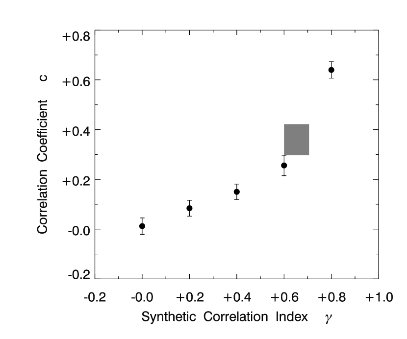
Figure 5: Comparison of our fitted correlation coefficient $c$ with $\gamma$, the imposed degree of correlation in the synthetic dataset. The gray area indicates the region in which the Pleiades most likely falls.

Our general result was that the predicted $\boldsymbol{y}$ still reproduced well the synthetic $\phi(m)$. The binary fraction $b$ was similarly accurate. Most significantly, the predicted $c$-value tracked the input quantity $\gamma$. Figure 5 shows this relation. We conclude that our statistical model, while crudely accounting for correlation by inserting a fraction of equal-mass pairs, nevertheless mimics a smoother correlation, such as would be found naturally. The shaded patch in the figure is the probable region occupied by the real Pleiades; Section 3.4 below justifies this assessment.

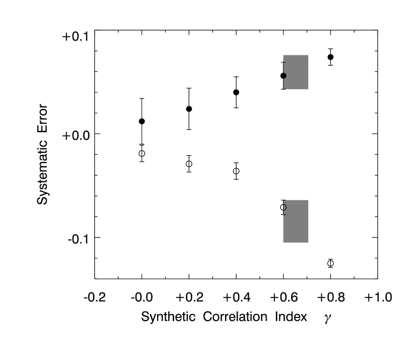
Figure 6: Systematic errors in parameters of the log-normal fit to $\phi(m)$, plotted as a function of the synthetic binary correlation $\gamma$. Filled circles show $\Delta m_{\circ}$, the error in $m_{\circ}$. Open circles show $\Delta\sigma_{m}$, the error in $\sigma_{m}$. The gray areas indicate the regions in which the Pleiades most likely falls.

One price we paid for our simplified account of correlation was that our matching of $\phi(m)$ was less accurate than for randomly paired input binaries. Consider, for example, the log-normal function of equation (41). While our best-fit $\boldsymbol{y}$ still reproduced $\phi(m)$ reasonably well, the output function peaked at too high a mass compared to $m_{\circ}$. The filled circles in Figure 6 shows that this shift, $\Delta m_{\circ}$, increased with the input $\gamma$-value. Concurrently, our output function was too narrow compared to the input $\sigma_{m}$. The (negative) difference, $\Delta\sigma_{m}$, displayed as open circles in Figure 6, was also more pronounced at higher $\gamma$. These systematic errors need to be considered when analyzing a real cluster. The two patched areas in the figure again represent the likely regime of the Pleiades, as we explain shortly.

3.3 Empirical Mass Distributions

We now present the results of applying our maximum likelihood analysis to the Pleiades itself, i.e., to the $I$- and $K$-magnitudes of 1245 sources from the catalog of Stauffer et al. (2007). Our best-fit binary fraction was $b\,=\,0.68\,\pm\,0.02$, while the correlation coefficient was $c\,=\,0.36\,\pm\,0.06$. (These and other uncertainties represent only random statistical error, and do not include systematic effects; see Section 5.) We will discuss the implications of these findings in the following section. First, we examine the global distribution of stellar mass.

The data points in Figure 7 are the best-fit values of each $y_{i}/\Delta m_{i}$. As in Figure 3, these points are a discrete representation of the single-star mass function $\phi(m)$. The large error bars on the two points at highest mass are due to the small number of sources gauged to be in the respective bins. The smooth, solid curve in Figure 7 is a log-normal mass function that best matches the empirical $\boldsymbol{y}$. Referring again to equation (41), we find that $m_{\circ}\,=\,0.20\,\pm\,0.04$ and $\sigma_{m}\,=\,0.38\,\pm\,0.02$. The presence of a finite binary correlation affects both estimates. Judging from Figure 6, our $m_{\circ}$ is overestimated by about 0.06, while $\sigma_{m}$ should be raised by 0.08.

Each of our mass bins has contributions from both the primary and secondary components of binary pairs, as quantified by equation (4). Integrating the full stellar mass probablity $\Phi(m_{p},m_{s})$ over all secondary masses, we obtain $\phi_{p}(m_{p})$, the probability distribution of primary masses:

$$\phi_{p}(m_{p})\,=\,\int_{0}^{m_{p}}\!dm_{s}\,\Phi(m_{p},m_{s})\,\,.$$ (43)

Note that this distribution includes the possibility that the star is single ($m_{s}\,=\,0$).

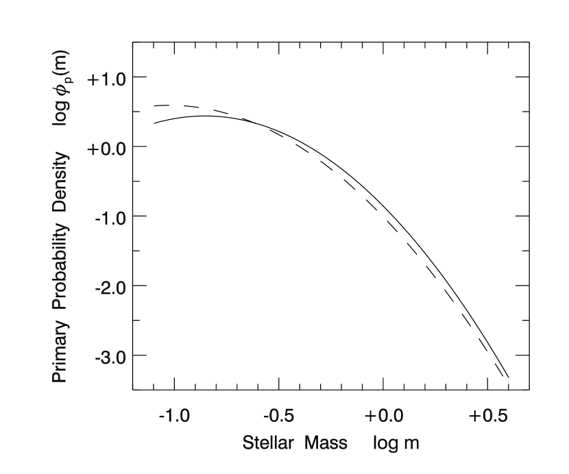
Figure 8: Comparison of log-normal fits to the primary probability density ${\rm log}\,\phi_{p}(m_{p})$ (solid curve) and the single star probability density ${\rm log}\,\phi(m)$ (dashed curve). The primary function peaks at larger mass and has a smaller width. Note that $\phi_{p}(m)$ includes single stars.

The solid curve in Figure 8 is a log-normal fit to the empirical $\phi_{p}(m_{p})$. Shown for comparison as a dashed curve is the fit for $\phi(m)$ from Figure 7. Relative to the latter function, the primary distribution falls off at lower masses. This falloff simply reflects the fact that less massive objects are more likely to be part of a binary containing a higher-mass star, and thus to be labeled as “secondaries.” In any event, we now see why the peak of $\phi_{p}(m_{p})$, $m_{\circ}\,=\,0.27\,\pm\,0.02$, is elevated with respect to the peak of $\phi(m)$. Similarly, the primary distribution is also slightly narrower than the single-star mass function, with $\sigma_{m}\,=\,0.35\,\pm\,0.01$.

The parameters of our log-normal approximation to $\phi_{p}(m_{p})$ may be compared to those of Moraux et al. (2004). These authors fit the entire mass function. Since, however, they did not account for binarity, their results are more closely analogous to our primary distribution. Their best-fit $m_{\circ}$ of 0.25 is close to ours, while their $\sigma_{m}$ of 0.52 is higher, mostly because of their inclusion of the highest-mass members. These parameters are also close to those given by Chabrier (2003) in his log-normal fit to the field-star initial mass function ($m_{\circ}\,=\,0.22$, $\sigma_{m}\,=\,0.57$).

In Figure 9, we compare our single-star distribution $\phi(m)$ to the field-star initial mass function (dashed curve). The latter, which has been raised in the figure for clarity, is taken from Kroupa (2001), who did correct for binarity. It is apparent that $\phi(m)$ itself veers away from the IMF for both low- and high-mass objects. When these are added in, the resemblance improves. The open circles in Figure 9 are Pleiades low-mass stars and brown dwarfs found by Bihain et al (2006). We have normalized their data, taken from a limited area of the cluster, so that their total number of stars matches ours within the overlapping mass range. No such normalization was necessary for the 11 B-type stars (filled circles), which are from the catalog of Stauffer et al. (2007) but not included in our maximum likelihood analysis. Adding both these groups not only improves the match to the IMF, but also reveals a gap in the stellar distribution between about 2 and $5\,\,M_{\odot}$. A similar gap is seen in the Pleiades mass function of Moraux et al. (2004, see their Figure 1).

Our estimate for the total cluster mass, based solely on the 1245 catalog sources, is $738\,\,M_{\odot}$, with a 4% uncertainty. Adding in the brightest stars brings this total to $820\,\,M_{\odot}$, with the same relative error. Tests with synthetic data indicate that the systematic bias due to binary correlation raises this figure by roughly $50\,\,M_{\odot}$, to $870\,\,M_{\odot}$. Addition of the brown dwarfs would cause a further, relatively small, increase. For comparison, Pinfield et al. (1998) found $735\,\,M_{\odot}$ in stars, and an upper limit of $131\,\,M_{\odot}$ for the brown dwarf contribution. Raboud & Mermilliod (1998) used the virial theorem to estimate a total mass of $720\,\,M_{\odot}$, with a 28% uncertainty. Direct integration of their mass function gave $950\,\,M_{\odot}$, with an 18% fractional error.

3.4 Binarity

The global binary fraction, $b\,=\,0.68$, obtained in our analysis represents most, but not all, of the full binary population. Omitted here are spatially resolved systems. For these, the primary and secondary appear as separate sources in the catalog of Stauffer et al. (1998). Counting resolved pairs raises the total fraction to about 76%, as we now show.

The smallest angular separation between stars in the catalog is $10^{\prime\prime}$. At the Pleiades distance of 133 pc, the corresponding physical separation is 1400 AU. An edge-on circular binary of exactly this orbital diameter will still be unresolved, since the components spend most of their time closer together. The true minimum separation in this case is 2200 AU. Here, we have divided 1400 AU by $2/\pi$, which is the average of ${|\rm sin}\,\theta|$, for $\theta$ randomly distributed between 0 and $2\pi$.

Of course, only a relatively small fraction of binaries have separations exceeding 2200 AU. The average total mass of our unresolved systems is $0.71\,\,M_{\odot}$. A binary of that total mass and a 2200 AU diameter has a period of $1.2\times 10^{5}\,\,{\rm yr}$. What fraction of binaries have even longer periods? Our average primary mass is $0.46\,\,M_{\odot}$, corresponding to a spectral type of M1. Fischer & Marcy (1992) studied the period distribution of binaries containing M-type primaries. They claimed that this distribution was indistinguishable from that found by Duquennoy & Mayor (1991) for G-type primaries. In this latter sample, 11% of the systems had periods greater than our limiting value. If the Pleiades periods are similarly distributed, then the total fraction of binaries - both resolved and unresolved - becomes $0.66/(1-0.11)\,=\,0.76$.

Even without this augmentation, our total binary fraction appears to be inconsistent with the available direct observations of the Pleiades. Thus, Bouvier et al. (1997) found visual pairs with periods between 40 and $3.4\times 10^{4}$ yr. Using the period distribution of Duquennoy & Mayor (1991) to extrapolate their observed binary fraction of 28% yields a total fraction of 60%. Mermilliod et al. (1992) observed spectroscopic pairs with periods under 3 yr. A similar exercise again yields 60%. We note, however, that this ostensible concurrence of results is based on very broad extrapolations from limited data. (See Fig. 4 of Bouvier et al. (1997).)

Our derived binary fraction also exceeds that found in the field-star population. Duquennoy & Mayor (1991) found that 57% of G stars are the primaries of binary or higher-order systems. Note that our $b$ represents the total probability that a star is in a binary, whether as the primary or secondary component. Since G stars are rarely secondaries, the comparison with Duquennoy & Mayor (1991) is appropriate. On the other hand, M stars are frequently secondaries, so we would expect the fraction of binaries with M-type primaries to be reduced. Lada (2006) has found that only 25% of M-stars are the primary components of binaries. Our own analysis yields a binary fraction of 45% for M-star primaries, still in excess of the field-star result.

If our finding of a relatively high binary fraction proves robust, it may provide a clue to the progenitor state of the Pleiades and other open clusters. A similar statement applies to the correlation between component masses within binaries. Our adopted method of gauging this correlation - inserting a fraction of equal-mass pairs in the mass function - is admittedly crude. Nevertheless, the strong result ($c\,=\,0.36\,\pm\,0.06$) is significant. Referring back to Figure 5, we find that the Pleiades correlation is equivalent to setting $\gamma$ equal to about 0.65 in the alternative description of equation (42). Whatever the origin of the Pleiades binaries, the primaries and secondaries were not formed by completely independent processes.

4 Application to the Pleiades: Radial Distributions

4.1 Number and Mass Profiles

We now employ the procedure outlined in Section 2.4 to investigate both the surface and volumetric density as a function of the projected distance from the cluster center. The filled circles in Figure 10, along with the associated error bars, represent the surface number density of sources, measured in pc^-2. The solid curve is a density profile using the empirical prescription of King (1962). Here, the core radius is 2.1 pc, while the tidal radius is 19 pc. For comparison, Adams et al. (2001) also fit the surface number density profile of their low-mass stars to a King model, with a core radius of 2.3-3.0 pc. Our profile is also at least roughly consistent with the cumulative number distribution displayed by Raboud & Mermilliod (1998). Our best-fit tidal radius is slightly larger than the 17 pc cited by these authors.

The surface mass density is plotted in an analogous fashion, again as a function of the projected radius. We show both the data points (small open circles) and, as the dashed curve, the best-fit King model. Here, the core radius is 1.3 pc, and the tidal radius is 18 pc. Note that the mass density profile falls off more steeply than the number density. Thus, stars near the center are abnormally massive, a trend we shall explore more extensively below.

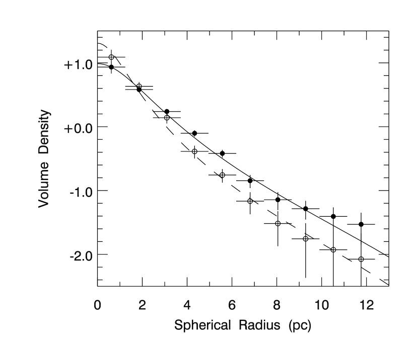
Figure 11: Volume density profiles. The filled circles represent the number density (${\rm pc}^{-3}$), again displayed logarithmically. Open circles are the mass density, in $M_{\odot}\,\,{\rm pc}^{-3}$. The solid and dashed smooth curves are the same King model fits as in Figure 10, but now deprojected into three-dimensional space.

Figure 11 displays the corresponding volumetric densities. As we indicated, the deconvolution from surface profiles assumes spherical symmetry. In fact, the Pleiades is slightly asymmetric, with a projected axis ratio of 1.2:1 (Raboud & Mermilliod, 1998). This ellipticity is thought to stem from the tidal component of the Galactic gravitational field (Wielen, 1974). Under the spherical assumption, the filled circles and solid, smooth curve show the number density. Here, the King model is the same used for the surface number density in Figure 10, but deprojected into three-dimensional space.

Figure 11 also shows, as the small open circles and dashed curve, the mass density as a function of spherical radius. Again, the King model here is the deprojected version of that from Figure 10. The relatively rapid falloff in the mass, as opposed to the number, density is another sign of the tendency for more massive stars to crowd toward the center.

The information we used in obtaining these profiles also gives us the spatial variation of the binary fraction $b$. That is, we first used equation (37) to obtain $\boldsymbol{\mu}^{r}$, the predicted mass distribution in each radial annulus. Recall that the distribution refers to both primaries and secondaries, as well as single stars. The binary fraction can thus be computed locally. To within our uncertainty, about $\pm 0.05$ at each radial bin, we find no variation of $b$ across the cluster.

4.2 Mass Segregation

We have mentioned, in a qualitative manner, that more massive cluster members tend to reside nearer the center. In Figure 12, we explicitly show this trend. Here, we plot $\langle m_{p}+m_{s}\rangle$, the average system mass (primary plus secondary) as a function of the projected cluster radius. It is apparent that $\langle m_{p}+m_{s}\rangle$ monotonically falls out to about 4 pc. Beyond that point, the average mass is roughly constant.

The pattern here is consistent with mass segregation, but is not a clear demonstration of that effect. The problem is that Figure 12 gives no indication of the relative populations at different annuli. If the outer ones are occupied by only a small fraction of the cluster, is mass segregation present? To gauge any variation in the mass distribution of stars, that distribution must be calculated over an adequate sample size.

Previous authors have also claimed evidence of mass segregation, using various criteria. Adams et al. (2001) looked at the distribution of surface and volumetric number densities for a number of different mass bins. Raboud & Mermilliod (1998) divided the population by magnitude into relatively bright and faint stars. They calculated the cumulative number as a function of radius for both groups, and found the bright stars to be more centrally concentrated. Finally, Pinfield et al. (1998) fit King profiles to the surface density of various mass bins. As the average mass increases, the core radius shrinks.

Figure 13 gives a simpler and more clear-cut demonstration of the effect. Here, we consider $f_{N}$, the number of sources enclused in a given projected radius, divided by the total number of sources in the cluster. We also consider $f_{M}$, the analogous fractional mass inside any projected radius. The figure then plots $f_{M}$ versus $f_{N}$. In the absence of mass segregation, $f_{M}$ would equal $f_{N}$ at each annulus. This hypothetical situation is illustrated by the dotted diagonal line.

In reality, $f_{M}$ rises above $f_{N}$, before they both reach unity at the cluster boundary (see upper smooth curve, along with the data points). This rise, as already noted, indicates that the innermost portion of the cluster has an anomalously large average mass, i.e., that mass segregation is present. Moreover, the area between the solid and dotted curves is a direct measure of the effect. In the case of “perfect” mass segregation, a few stars near the center would contain virtually all the cluster mass. The solid curve would trace the upper rectangular boundary of the plot, and the enclosed area would be 0.5. We thus define the Gini coefficient, $G$, as twice the area between the actual $f_{M}-f_{N}$ curve and the central diagonal. For the Pleiades, we find that $G\,=\,0.20\pm 0.06$.

It is possible, at least in principle, that this effect is due entirely to a few exceptionally massive stars located near the center. In fact, this is not the case. We have artificially removed the 11 brightest sources (all late-B stars) and recalculated $f_{M}$ versus $f_{N}$. The result is shown by the dashed curve in Figure 13. While the rise above the diagonal is diminished, it is still present. That is, the intermediate-mass population exhibits segregation, as well.

An interesting contrast is presented by another populous group, the Orion Nebula Cluster (ONC). The distribution of stellar masses in this far younger system was recently studied by Huff & Stahler (2006). Figure 2 in that paper compares the stellar populations in the inner and outer halves of the cluster. Apart from a few high-mass objects, the two populations are essential identical.

We may also construct an $f_{M}-f_{N}$ curve for the ONC, as shown here in Figure 14. The solid curve again lies well above the fiducial diagonal, ostensibly indicating mass segregation. However, removal of just the four Trapezium stars gives a dramatically different result (dashed curve) that is virtually indistinquishable from the diagonal. All stars except this tiny subset are similarly distributed. The cluster is too young to have undergone true mass segregation, a conclusion drawn previously from N-body simulations (Bonnell & Davies, 1998). The Trapezium represents a special population, one that probably formed just prior to cloud dispersal (Huff & Stahler, 2007).

5 Discussion

In this paper, we have applied a versatile statistical tool, the maximum likelihood technique, to assess the distribution of stellar mass and the incidence of binaries in the Pleiades. We began with a near-infrared catalog of cluster members. Our basic assumption was that all cluster members share the same evolutionary age, and that any dispersion in the color-magnitude plane stems from binarity and random photometric errors. We were then able to infer the most probable distribution of masses, both for the cluster as a whole, and as a function of distance from its center. Finally, we introduced a simple method for gauging the degree of mass segregation in the cluster.

One of our surprising results is the relatively high fraction of binaries. We estimate that 68% of all systems in the cluster are unresolved binaries; this figure climbs to about 76% if resolved pairs are included. These fractions are significantly higher than the accepted field-star result, so we should scrutinize them carefully. Could they stem from an underestimate of the photometric error at faint magnitudes? Since the error in $I$ is greater than $K$, we artificially increased the dispersion $\sigma_{I}$. We kept $\sigma_{I}$ at 0.15 until $M_{I}\,=\,9.5$, below which we increased it linearly, reaching $\sigma_{I}\,=\,0.20$ at $M_{I}\,=\,12$. After redoing the maximum likelihood analysis, the global binary fraction $b$ for unresolved pairs is unchanged.

Another potential difficulty is our neglect of the physical thickness of the cluster. We have assigned all members a distance of 133 pc, although there will naturally be some variation. However, this effect is also relatively small. From Section 4.1, the volumetric number density falls off with radius approximately as a King model with core and tidal radii of 2.1 and 19 pc, respectively. Consider the front half of a spherical cluster with such a density distribution. It may readily be shown that the mean distance from the plane of the sky of any cluster member is $d\,=\,2.6\,{\rm pc}$. For a cluster at mean distance $D$, the induced magnitude spread is $5\ {\rm log}\,[(D+d)/D]$, which is 0.04 in our case. Although the actual spread in magnitudes is not Gaussian, we have added this figure in quadrature to both $\sigma_{I}$ and $\sigma_{K}$, and rerun the analysis. Again, the binarity is unaffected.

The errors due to both photometry and finite cluster thickness induce a symmetric spread in stellar magnitudes. That is, they scatter as many sources below the fiducial isochrone as above it. Thus, they cannot reduce the estimated binarity, which stems from an excess of stars above the isochrone. One systematic error that would affect $b$ is an overestimation of the cluster distance. If $D$ were lowered, the absolute magnitudes of all sources would decrease equally, as would the inferred $b$-value. Quantitatively, the distance would have to decrease by about 15 pc to bring the binary fraction down to the field-star result for G-dwarf primaries. An error of this size for the average distance is excluded by current observations, for which the estimated uncertainty is only 1 pc (Soderblom et al., 2005).

Since our method relies solely on photometry to assess binarity, we cannot distinguish between physically linked pairs and chance alignments. As mentioned in Section 3.4, the resolution limit of our data is $10^{\prime\prime}$, or $\Delta r_{\circ}\,=\,1400~{}{\rm AU}$ at the distance of the Pleiades. Consider a star at a radius $r$ from the cluster center. Its average number of neighbors within $\Delta r_{\circ}$ is $\pi\,\Delta r_{\circ}^{2}\,n_{s}(r)$,where $n_{s}(r)$ is the projected surface number density of the cluster. Since each ring of width $dr$ contains $2\,\pi\,n_{s}\,r\,dr$ stars, integration over all members yields the total number of chance alignments:

$$N_{\rm chance}\,=\,2\,\pi^{2}\,\Delta r_{\circ}^{2}\int_{0}^{R}\!n_{s}^{2}(r)\,r\,dr\,\,.$$ (44)

where $R$ is the cluster’s outer radius, Using $n_{s}(r)$ from Figure 10, we find$N_{\rm chance}\,=\,2.4$. Thus, chance alignments have no quantitative impact.

Yet another source of systematic error is the cluster age. We have adopted the lithium-based figure of 125 Myr from Stauffer et al. (1998). Earlier estimates, using the main-sequence turnoff, yielded a range of answers. For example, Meynet et al. (1993) found 100 Myr. Even this minor reduction affects our results, since it lifts the low-mass end of the isochrone toward higher luminosity. For an age of 100 Myr, our analysis gives $b\,=\,0.57\,\pm\,0.02$ and $c\,=\,0.28\,\pm\,0.06$. The binary fraction is augmented to 0.64 when we include resolved pairs. From Figure 3 of Stauffer et al. (1998), a 100 Myr age corresponds to a lithium edge at $M_{I}\,=\,11.7$, or $I\,=\,17.3$ at the Pleiades distance. Such a result seems incompatible with the lithium data shown in Figure 2 of Stauffer et al. (1998), but the total number of observations is relatively small.

We conclude that the enhanced binarity is a real effect. What this fact tells us about the origin of open clusters remains to be seen. Our next step in addressing this basic issue is to try and account theoretically for the empirical properties just obtained through our statistical analysis. We will ascertain, using direct numerical simulations, the range of initial states that can relax dynamically to the present-day Pleiades. Such a study will bring us one step closer to understanding the molecular cloud environments that give rise to open clusters.

Appendix A Interpreting the Gini Coefficient

In Section 4.2, we introduced the Gini coefficient geometrically, as twice the area between the $f_{M}-f_{N}$ curve and the diagnonal line representing zero mass segregation. Alternatively, $G$ may be defined in terms of the mean mass difference between radial shells in the cluster. Here we describe more precisely, and prove the equivalence of, this second interpretation.

Altering our previous notation, we now let $m(r)$ be the average system mass (primary plus secondary) in a shell with outer radius $r$. If there are many shells, then we may define a system number density $n(r)$, such that the number of systems between $r$ and $r+dr$ is $n(r)\,dr$. The total number of systems at all radii is

$$N_{\rm tot}\,=\,\int_{0}^{\infty}\!n(r)\,dr\,\,.$$ (A1)

This total was called $\mu_{\rm tot}$ in the text. The average system mass throughout the entire cluster is

$${\bar{m}}\,=\,\frac{1}{N_{\rm tot}}\int_{0}^{\infty}\!m(r)\,n(r)\,dr\,\,.$$ (A2)

We will be concerned with the relative mean difference in the mass of shells. This is

$${\bar{\Delta}}\,=\,\frac{1}{{\bar{m}}\,N_{\rm tot}^{2}}\int_{0}^{\infty}\!dr\int_{0}^{\infty}\!dr^{\prime}\,{|m(r)\,-\,m(r^{\prime})|}\,\,n(r)\,\,n(r^{\prime})\,\,.$$ (A3)

We will prove that the Gini coefficient, as defined in Section 4.2, is also $\bar{\Delta}/2$.

In the geometric definition of $G$, we utilized the cumulative fractional number $f_{N}$ and cumulative fractional mass $f_{M}$. These may be written in terms of the system number density:

$$f_{N}(r) = \frac{1}{N_{\rm tot}}\int_{0}^{r}\!n(r^{\prime})\,dr^{\prime}\,\,,$$ (A4)

$$f_{M}(r) = \frac{1}{{\bar{m}}\,N_{\rm tot}}\int_{0}^{r}\!m(r^{\prime})\,n(r^{\prime})\,dr^{\prime}\,\,.$$ (A5)

We will later need the differentials of $f_{N}$ and $f_{M}$, which are

$${df}\!_{N} = \frac{n(r)}{N_{\rm tot}}\,\,dr\,\,,$$ (A6)

$${df}\!_{M} = \frac{m(r)\,n(r)}{{\bar{m}}\,N_{\rm tot}}\,\,\,dr\,\,.$$ (A7)

In terms of $f_{N}$ and $f_{M}$, the geometric definition of $G$ is then

$$G\,=\,2\int_{0}^{1}\!\left(f_{M}\,-\,f_{N}\right)\,df_{N}\,\,.$$ (A8)

If the mass is centrally concentrated, as expected in a real stellar cluster, then $f_{M}\,\geq\,f_{N}$ at all radii, and $G\,\geq\,0$. Hypothetical clusters in which larger masses are preferentially located farther from the center would have $G\,\leq\,0$.

We now return to equation (A3) and manipulate it to obtain $G$, as defined above. A central assumption we will make is that $m(r)$ declines monotonically with $r$. We may then expand the righthand side of equation (A3). We split the integral over $r^{\prime}$ into two parts, one for $r^{\prime}\leq r$ and the other for $r^{\prime}>r$. Under our assumption, $m(r^{\prime})\,\geq\,m(r)$ in the first integral, and $m(r^{\prime})\,<\,m(r)$ in the second. After pulling $n(r)$ from the $r^{\prime}$-integration, we further split the integrands to find

$${\bar{\Delta}}\,=\,\frac{1}{{\bar{m}}\,N_{\rm tot}}\int_{0}^{\infty}\!(-{\cal I}_{1}\,+\,{\cal I}_{2}\,+\,{\cal I}_{3}\,-\,{\cal I}_{4})\,\,n(r)\,dr\,\,.$$ (A9)

The first two terms of the integrand are

$${\cal I}_{1} \equiv \frac{m(r)}{N_{\rm tot}}\int_{0}^{r}\!n(r^{\prime})\,dr^{\prime}\,=\,m(r)\,f_{N}(r)\,\,,$$ (A10)

$${\cal I}_{2} \equiv \frac{1}{N_{\rm tot}}\int_{0}^{r}\!m(r^{\prime})\,n(r^{\prime})\,dr^{\prime}\,=\,{\bar{m}}\,f_{M}(r)\,\,.$$ (A11)

The third term is

$${\cal I}_{3} \equiv \frac{m(r)}{N_{\rm tot}}\int_{r}^{\infty}\!n(r^{\prime})\,dr^{\prime}$$ (A12)

$$= \frac{m(r)}{N_{\rm tot}}\int_{0}^{\infty}\!n(r^{\prime})\,dr^{\prime}\,-\,\frac{m(r)}{N_{\rm tot}}\int_{0}^{r}\!n(r^{\prime})\,dr^{\prime}$$ (A13)

$$= m(r)\,-\,m(r)\,f_{N}(r)\,\,,$$ (A14)

while the fourth is

$${\cal I}_{4} \equiv \frac{1}{N_{\rm tot}}\int_{r}^{\infty}\!m(r^{\prime})\,n(r^{\prime})\,dr^{\prime}$$ (A15)

$$= \frac{1}{N_{\rm tot}}\int_{0}^{\infty}\!m(r^{\prime})\,n(r^{\prime})\,dr^{\prime}\,-\,\frac{1}{N_{\rm tot}}\int_{0}^{r}\!m(r^{\prime})\,n(r^{\prime})\,dr^{\prime}$$ (A16)

$$= {\bar{m}}\,-\,{\bar{m}}\,f_{M}(r)\,\,.$$ (A17)

Putting equations (A10), (A11), (A14), and (A17) back into equation (A9) yields

$$\bar{\Delta} = \frac{1}{{\bar{m}}\,N_{\rm tot}}\int_{0}^{\infty}\!\left[2\,{\bar{m}}\,f_{M}(r)\,-\,2\,m(r)\,f_{N}(r)\,+\,m(r)\,-\,{\bar{m}}\right]\,n(r)\,dr$$ (A18)

$$= 2\,\left(\int_{0}^{1}\!f_{M}\,df_{N}\,-\,\int_{0}^{1}\!f_{N}\,df_{M}\right)\,\,,$$ (A19)

where we have used both equations (A1) and (A2) to cancel the last two terms on the right side of equation (A18), and equations (A6) and (A7) to transform the remaining two terms. The second integral in the last equation is

$$\int_{0}^{1}\!f_{N}\,df_{M} = \int_{f_{N}f_{M}=0}^{f_{N}f_{M}=1}\!d\,(f_{N}f_{M})\,-\,\int_{0}^{1}\!f_{M}\,df_{N}$$ (A20)

$$= 1\,-\,\int_{0}^{1}\!f_{M}\,df_{N}\,\,,$$ (A21)

since $f_{M}$ and $f_{N}$ attain their upper and lower bounds simultaneously. Using this result, equation (A19) becomes

$${\bar{\Delta}}\,=\,2\,\left(2\int_{0}^{1}\!f_{M}\,df_{N}\,-\,1\right)\,\,.$$ (A22)

Finally, we note that

$$2\int_{0}^{1}\!f_{N}\,df_{N}\,=\,1\,\,.$$ (A23)

Thus, equation (A22) becomes

$${\bar{\Delta}} = 4\,\left(\int_{0}^{1}\!f_{M}\,df_{N}\,-\,\int_{0}^{1}\!f_{N}\,df_{N}\right)$$ (A24)

$$= 4\int_{0}^{1}\!\left(f_{M}\,-\,f_{N}\right)\,df_{N}$$ (A25)

$$= 2\,G\,\,,$$ (A26)

as claimed.

Figure 1: Near-infrared color-magnitude diagram for the Pleiades. Small dots represent the 1245 stars in our sample. Open circles are the 41 likely sub-stellar objects which have been removed from the sample. Filled circles are the 11 brightest stars, which are likely post-main-sequence objects. The 125 Myr isochrone for stars with masses between 0.08 and 4.0  $M_{\odot}$ is shown as the smooth, solid curve.

Figure 2: Observational error in the $K$-band measurements as a function of absolute magnitude for all 1417 stars in the catalog of Stauffer et al. (2007). The smooth curve is the approximate fit used in our maximum likelihood analysis.

Figure 3: Sample synthetic data results for the single star mass function $\phi(m)$. In both panels, the smooth curve is the input function from which the synthetic data were drawn. Shown also are the best-fit values, along with errors, for our discrete representation of the function. In the left panel, the input $\phi(m)$ is a power law with slope -2.8; in the right panel, it is a log-normal function with peak $m_{\circ}=0.2$ and width $\sigma_{m}\,=\,0.4$.

Figure 4: Weighted sum of the biases as a function of the regularization parameter $\lambda$. The synthetic input here was a log-normal function with 1245 sources. The dashed, horizontal line is drawn at $\chi_{b}^{2}\,=\,N$, where $N\,=\,21$ is the number of free parameters in our fitting. The short, vertical arrow indicates the final value of $\lambda$ used for this synthetic dataset.

Figure 7: Best-fit single star probability density $\phi(m)$ for the Pleiades. Actual bin values $y_{i}/\Delta m_{i}$ are shown with associated errors. The smooth curve is a log-normal approximation to the results.

Figure 9: Comparison of the Pleiades single star probability density to the field-star initial mass function of Kroupa (2001), where the latter has been shifted upward for clarity. Shown here is the log-normal approximation to ${\rm log}\,\phi(m)$ (solid curve), augmented with the data of Bihain et al (2006) for low-mass members and brown dwarfs (open circles) and our 11 brightest, post-main-sequence stars (filled circles).

Figure 10: Surface density distribution in the Pleiades. The filled circles represent the surface number density (${\rm pc}^{-2}$), displayed on a logarithmic scale. Open circles are the mass density, in $M_{\odot}\,\,{\rm pc}^{-2}$. The solid and dashed smooth curves are King model fits.

Figure 12: Average system mass (primaries plus secondaries) as a function of projected cluster radius. The bins here have constant radial width.

Figure 13: Fractional mass versus fractional number for the Pleiades. The data points and error bars, along with the solid curve, utilize all sources in the catalog of Stauffer et al. (2007). The dashed curve shows the result when the 11 brightest stars are removed. In both cases, the radial bins contain roughly equal numbers of stars. Finally, the dotted diagonal is the hypothetical result for no mass segregation.

Figure 14: Fractional mass versus fractional number for the ONC. The solid curve was computed using all the ONC sources analyzed by Huff & Stahler (2006). The dashed curve shows the result if only the 4 Trapezium stars are removed. As in Figure 13, the radial bins contain roughly equal numbers of stars. The dotted diagonal again shows the hypthetical condition of no mass segregation.

References

- Adams et al. (2001) Adams, J. D., Stauffer, J. R., Monet, D. G., Skrutskie, M. F & Beichman, C. A. 2001,AJ, 121, 2053
- Baraffe et al (1998) Baraffe, I., Chabrier, G., Allard, F., & Hauschildt, P. H. 1998, A&A, 337,403
- Bihain et al (2006) Bihain, G. et al. 2006, A&A, 458, 805
- Binney & Merrifield (1998) Binney, J. & Merrifield, M. Galactic Astronomy, Princeton: Princeton U. Press
- Bonnell & Davies (1998) Bonnell, I. A. & Davies, M. B. 1998, MNRAS, 298, 93
- Bouvier et al. (1997) Bouvier, J., Rigaut, F. & Nadeau, D. 1997, A&A, 323, 139
- Brown (2001) Brown, A. G. A. 2001, Rev. Mexicana Astron. Astrofis., 11, 89
- Chabrier (2003) Chabrier, G. 2003, PASP, 115, 763
- Cohen et al. (2003) Cohen, M., Wheaton, M. A., & Megeath, S. T. 2003, AJ, 126, 1090
- Cowen (1998) Cowen, G. 1998, Statistical Data Analysis, Oxford: Oxford U. Press
- Deacon & Hambly (2004) Deacon, N. R. & Hambly, N. C. 2004, A&A, 416, 125
- de La Fuente Marcos (1996) de La Fuente Marcos, 1996, A&A, 314, 453x
- Dias et al. (2002) Dias, W.S., Alessi, B.S., Moitinho, A., & Lepine, J.R.D. 2002, A&A, 389, 871
- Duquennoy & Mayor (1991) Duquennoy, A. & Mayor, M. 1991, A&AS, 88, 241
- Fischer & Marcy (1992) Fischer, D. A. & Marcy, G. W. 1992, ApJ, 396, 178
- Garcia & Mermilliod (2001) Garcia, B. & Mermilliod, J. C. A&A, 368, 122
- Haisch et al. (2004) Haisch, K. E., Greene, T. P., Barsony, M. & Stahler, S. W. 2004, AJ, 127, 1747
- Hambly et al. (1993) Hambly, N. C., Hawkins, M. R. S. & Jameson, R. F. 1993, A&AS, 100, 607
- Hoffleit et al. (1991) Hoffleit, D. et al. 1991, Bright Star Catalogue, New Haven: Yale University Press
- Huff & Stahler (2006) Huff, E. H. & Stahler, S. W. 2006, ApJ, 644, 355
- Huff & Stahler (2007) Huff, E. H. & Stahler, S. W. 2007, ApJ, 666, 281
- King (1962) King, I. 1962, AJ, 67, 471
- Kroupa (2001) Kroupa, P. 2001, MNRAS, 322, 231
- Lada (2006) Lada, C. J. 2006, ApJ, 640, 63
- Mason et al. (1998) Mason, B. D., Henry, T. J., Hartkopf, W. I., Ten Brummelaar, T. & Soderblom, D. R. 1998, AJ, 116, 2975
- Mermilliod et al. (1992) Mermilliod, J.-C., Rosvick, J. M., Duquennoy, A. & Mayor, M. 1992, A&A, 265, 513
- Meynet et al. (1993) Meynet, G., Mermilliod, J.-C., & Maeder, A. 1993, A&AS, 98, 477
- Moraux et al. (2003) Moraux, E., Bouvier, J., Stauffer, J. R., & Cuillandre, J.-C. 2003, A&A, 400, 891
- Moraux et al. (2004) Moraux, E., Kroupa, P., & Bouvier, J. 2004, A&A, 426, 75
- Palla & Stahler (2000) Palla, F. & Stahler, S. W. 2000, ApJ, 540, 255
- Pinfield et al. (1998) Pinfield, D. J., Jameson, R. F., & Hodgkin, S. T. 1998, MNRAS, 299, 955
- Pinfield et al. (2000) Pinfield, D. J., Hodgkin, S. T., Jameson, R. F., Cossburn, M. R., Hambly, N. C., & Devereux, N. 2000, MNRAS, 313, 347
- Pinfield et al. (2003) Pinfield, D. J., Dobbie, P. D., Jameson, R. F., Steele, I. A., Jones, H. R. A., & Katsiyannis, A. C. 2003, MNRAS, 342, 1241
- Press et al. (2002) Press, W. H., Teukolsky, S. A., Vetterling, W. T., & Flannery, B. P. 2002, Numerical Recipes in C: Second Edition, Cambridge: Cambridge U. Press
- Raboud & Mermilliod (1998) Raboud, D. & Mermilliod, J.-C. 1998, A&A, 329, 101
- Romani & Weinberg (1991) Romani, R. W. & Weinberg, M. D. 1991, ApJ, 372, 487
- Schwartz & Becklin (2005) Schwartz, M. J. & Becklin, E. E. 2004, AJ, 130, 2352
- Sen (1997) Sen, A. 1997, On Economic Inequality, Oxford: Clarendon Press
- Siess et al. (2000) Siess, L., Dufour, E., & Forestini, M. 2000, A&A, 358, 593
- Soderblom et al. (2005) Soderblom, D., Nelan, E., Benedict, G., McArthur, B., Ramirez, I., Spiesman, W., & Jones, B. 2005, AJ, 129, 1616
- Stauffer et al. (1998) Stauffer, J. R., Schultz, G, & Kirkpatrick, J. D. 1998, ApJ, 499, 199
- Stauffer et al. (2007) Stauffer, J. R. et al. 2007, ApJS, 172, 663
- Steele & Jameson (1995) Steele, I. A. & Jameson, R. F. 1995, MNRAS, 272, 630
- Tassis (2007) Tassis, K. 2007, MNRAS, 379, L50
- Wielen (1974) Wielen, R. 1974, in Stars and the Milky Way System, ed. L. N. Mavridis (Berlin: Springer-Verlag), p. 326
- Zinnecker & Mathieu (2001) Zinnecker, H. & Mathieu, R. D. (eds) 2001, The Formation of Binary Stars, San Francisco: ASP