Multigrid Hirsch-Fye quantum Monte Carlo method for dynamical mean-field theory

Abstract

We present a new algorithm which allows for direct numerically exact solutions within dynamical mean-field theory (DMFT). It is based on the established Hirsch-Fye quantum Monte Carlo (HF-QMC) method. However, the DMFT impurity model is solved not at fixed imaginary-time discretization $\Delta\tau$, but for a range of discretization grids; by extrapolation, unbiased Green functions are obtained in each DMFT iteration. In contrast to conventional HF-QMC, the multigrid algorithm converges to the exact DMFT fixed points. It extends the useful range of $\Delta\tau$, is precise and reliable even in the immediate vicinity of phase transitions and is more efficient, also in comparison to continuous-time methods. Using this algorithm, we show that the spectral weight transfer at the Mott transition has been overestimated in a recent density matrix renormalization group study.

Mott metal-insulator transitions and other effects of strong electronic correlations are among the most intriguing phenomena in solid state physics SCES . They occur when the effective electronic bandwidths of $d$ or $f$ shell electrons become comparable with the local Coulomb interactions. This most interesting regime is also most challenging: here, perturbative expansions (both at weak and at strong coupling) and effective independent-electron methods such as density functional theory DFT within local density approximation (LDA) break down.

Unfortunately, nonperturbative methods for a direct treatment of correlated lattice electrons are either restricted to one-dimensional (i.e., chain- or ladder-like) systems or suffer from severe finite-size and/or sign problems. However, a significant reduction of complexity in higher-dimensional cases is achieved by the dynamical mean-field theory (DMFT) which maps the electronic lattice problem onto an Anderson impurity model with a self-consistent bath; this mapping becomes exact in the limit of infinite lattice coordination Georges96 . Within the last 15 years, much insight into strongly correlated systems and phenomena has been gained using the DMFT. Many of these studies have relied on the Hirsch-Fye quantum Monte Carlo (HF-QMC) method Hirsch86 for solving the DMFT impurity problem at finite temperatures.

The HF-QMC method discretizes the imaginary-time path integral into slices of uniform width $\Delta\tau$ and employs a Trotter decoupling; this modified impurity problem is solved via Monte Carlo sampling of a binary Hubbard-Stratonovich field. In principle, arbitrary precision can be achieved using HF-QMC in the combined limit of infinitely many updates of the Hubbard-Stratonovich field and of vanishing discretization $\Delta\tau$; in this broader sense, HF-QMC is numerically exact. However, practical lower limits for the discretization exist (primarily due to a scaling of the numerical effort with $(\Delta\tau)^{-3}$ for fixed temperature $T$), so that raw HF-QMC results usually contain systematic Trotter errors which are much larger than the statistical Monte Carlo errors. This implies, in the DMFT context, that all observables and phase boundaries depend on the auxiliary parameter $\Delta\tau$ chosen in the self-consistency cycle. While high accuracy and efficiency have been demonstrated for a posteriori extrapolations $\Delta\tau\to 0$ of certain static observables Bluemeretc ; Bluemer07 , these procedures require special care and experience and may fail close to phase transitions. Up to recently, the Trotter bias of HF-QMC derived spectral functions could not be reduced at all.

For a long time, Trotter errors could only be avoided using fundamentally different impurity solvers that either introduce a logarithmic frequency discretization directly (numerical renormalization group, NRG) or represent impurity plus bath as a finite cluster or chain [exact diagonalization (ED), density-matrix renormalization group (DMRG)]. Consequently, their results, too, contain systematic finite-size/discretization errors; in particular, these alternatives to QMC yield continuous spectra only after numerical broadening. Only very recently, two new quantum Monte Carlo impurity solvers have become available Rubtsov05 ; Werner06 which are numerically exact in the stricter sense that their results are correct within statistical error bars, without the need for explicit extrapolations. These methods avoid the imaginary-time discretization of HF-QMC and rely, instead, on perturbative expansions in the interaction and hybridization, respectively, which are statistically sampled to arbitrary order. However, the continuous-time quantum Monte Carlo (CT-QMC) methods are often less efficient than HF-QMC Bluemer07 .

In this Letter, we propose a new algorithm for solving the DMFT self-consistency equations in quasi continuous imaginary time, based on a multigrid implementation of the HF-QMC method. This implementation removes many of the limitations of HF-QMC; in particular, it yields precise and reliable results even at phase boundaries. As a first application, we test DMRG predictions Karski05 of the spectral weight transfer at the Mott transition – a study that would not have been possible using conventional HF-QMC.

Multigrid HF-QMC method – Before we formulate the new multigrid approach, let us discuss the flow diagram Fig. 1(a) of the conventional HF-QMC method.

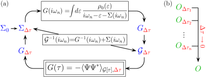
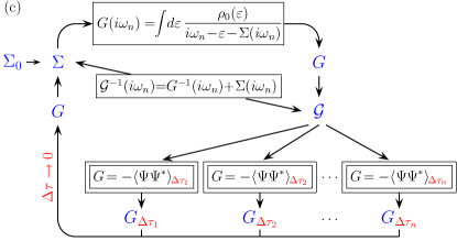
Figure 1: (Color online) (a) Conventional HF-QMC algorithm: Trotter error of impurity Green function $G$ (computed at fixed $\Delta\tau$) leads to bias in bath Green function ${\cal G}$, self-energy $\Sigma$, and all observables. (b) Extrapolation $\Delta\tau\to 0$ of observable O. (c) Multigrid HF-QMC scheme: DMFT iteration with unbiased impurity Green function, extrapolated from multiple HF-QMC solutions $G_{\Delta\tau_{1}}\dots G_{\Delta\tau_{n}}$: at self-consistency, $G$, ${\cal G}$, $\Sigma$, and all derived observables are numerically exact.

Starting with some guess $\Sigma_{0}$ for the self-energy, the lattice Green function $G$ is obtained via the lattice Dyson equation (upper box, here written for the 1-band Hubbard model); as a next step, the impurity Dyson equation (middle box) is used to determine the bath Green function ${\cal G}$ which defines the DMFT impurity problem (lower box). Conventionally, this is solved using HF-QMC at a fixed discretization; the resulting Green function closes the DMFT cycle via the impurity Dyson equation. Obviously, the Trotter error in the impurity solver affects the whole DMFT cycle; thus, at self-consistency, $G_{\Delta\tau}$, ${\cal G}_{\Delta\tau}$, $\Sigma_{\Delta\tau}$ and all observables deviate from their physical values, ideally with corrections in powers of $(\Delta\tau)^{2}$. Only then, numerically exact estimates of observables can be extrapolated a posteriori from results of independent HF-QMC DMFT runs, as illustrated in Fig. 1(b).

The new multigrid method, visualized in Fig. 1(c), splits the impurity-solving part of the DMFT self-consistency cycle into two steps: first, the impurity problem is solved – at fixed bath Green function ${\cal G}$ – for a suitable range of discretizations $\Delta\tau_{i}\in[\Delta\tau_{\text{min}},\Delta\tau_{\text{max}}]$ using HF-QMC. In a second step, a numerically exact estimate $G$ of the true Green function of the given impurity problem is obtained by extrapolation of the multiple resulting Green functions $G_{\Delta\tau_{i}}$. This highly nontrivial task is accomplished using a scheme developed recently (in the context of a posteriori extrapolation) Bluemer07a : (i) each of the discrete HF-QMC estimates is interpolated with the help of a suitably chosen reference model onto a common fine $\tau$ grid; (ii) quadratic (in $\Delta\tau^{2}$) least-squares extrapolations $\Delta\tau\to 0$ are performed on this grid. In practice, the raw Green functions $G_{\Delta\tau_{i}}$ are averaged over 10–20 impurity solutions. Thus, for about 10 discretizations $\Delta\tau_{i}$, the multigrid method parallelizes to about 100 CPU cores. For optimal accuracy, a hierarchy of discretization scales and high-frequency cut-offs needs to be maintained fn:parameters ; details will be presented elsewhere BluemerPrep . Since the multigrid algorithm closes the DMFT self-consistently with an impurity Green function that is (for correctly chosen parameters, see below) unbiased, all state variables $G$, ${\cal G}$, and $\Sigma$ converge to their numerically exact forms.

This fundamental advantage of the multigrid HF-QMC method is illustrated in the scheme Fig. 2:

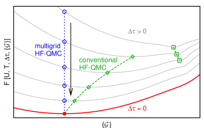
Figure 2: (Color online) Scheme: GL free energy in multidimensional space of hybridization functions $\{{\cal G}\}$. The fixed points of conventional HF-QMC (diamonds, squares) are adiabatically connected to the exact fixed point (full circle) only for small $\Delta\tau$. In contrast, the multigrid method solves all impurity problems at the $\Delta\tau=0$ fixed point (circles).

Here, the solid line depicts the exact Ginzburg-Landau (GL) free energy $F[U,T,\{{\cal G}\}]$ in the multi-dimensional space of bath Green functions $\{{\cal G}\}$ (for fixed physical parameters, $U$, $T$); its stationary points mark the DMFT fixed points Kotliar00 . However, conventional HF-QMC implementations converge to the stationary points (squares, diamonds) of generalized GL functionals (dotted lines) with additional dependence on $\Delta\tau$. These fixed points can vary irregularly or even discontinuously as a function of $\Delta\tau$ which complicates or prevents extrapolations $\Delta\tau\to 0$. In contrast, the multigrid HF-QMC procedure drives the DMFT iteration to the numerically exact fixed point: at self-consistency, each finite-$\Delta\tau$ HF-QMC evaluation is performed for the bath Green function at which $F[U,T,\{{\cal G}\}]$ is stationary (full circle) while the generalized functionals $F[U,T,\Delta\tau,\{{\cal G}\}]$ are not (empty circles).

Benchmark results – For a quantitative discussion, let us now consider the one-band Hubbard model with semi-elliptic density of states (bandwidth $W=4$) at low temperatures $T$ in the strongly correlated regime. Specifically, we will concentrate on the double occupancy $D=\langle n_{\downarrow}n_{\uparrow}\rangle$, an observable which is well-defined for the impurity model irrespective of DMFT self-consistency and which is best computed at fixed $\Delta\tau$ in both algorithms. Figure 3

Figure 3: (Color online) Double occupancy $D=\langle n_{\downarrow}n_{\uparrow}\rangle$ at $T=1/45$, $U=5$ for metallic (upper set of curves) and insulating (lower set of curves) phases: results from conventional HF-QMC (diamonds) and from multigrid HF-QMC (circles).

shows results for the coexisting metallic and insulating phases versus squared discretization at $T=1/45$ and interaction $U=5$. Conventional HF-QMC (diamonds) finds an insulating solution only for relatively small $\Delta\tau\lesssim 0.4$. While a metallic solution can be stabilized at arbitrarily large $\Delta\tau$, the $\Delta\tau$ dependence of $D$ is highly nonuniform which restricts the useful range for extrapolations $\Delta\tau\to 0$ (dashed lines), again, to small values $\Delta\tau\lesssim 0.4$. In contrast, the multigrid HF-QMC raw data (circles) shows regular $\Delta\tau$ dependence even at large discretizations which allows for very precise extrapolations (solid lines) based on cheap large-$\Delta\tau$ HF-QMC data fn:logD . Evidently, the multigrid method is superior.

However, such extrapolations, as well as all observable estimates that can be derived from the Green function and self-energy without explicit $\Delta\tau\to 0$ extrapolation, are only reliable if the multigrid algorithm has really converged to the exact DMFT fixed point. Thus, we have to check for any bias that might survive from the intrinsic parameters, most notably the range $[\Delta\tau_{\text{min}},\Delta\tau_{\text{max}}]$ used in the internal Green function extrapolation. In the inset of Fig. 4,

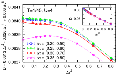
Figure 4: (Color online) Inset: multigrid HF-QMC results for double occupancy $D=\langle n_{\downarrow}n_{\uparrow}\rangle$ at $T=1/45$, $U=4$, using different ranges $[\tau_{\text{min}},\tau_{\text{max}}]$ in the Green function extrapolation. Main panel: same data minus leading $\Delta\tau$ corrections.

multigrid HF-QMC results (at $U=4$, i.e, in the metallic phase) are plotted for various $\Delta\tau$ grids; at this scale, both the raw data and the fit curves fall on top of each other. For a fine-scale analysis, the approximate leading Trotter errors have been subtracted in the main panel of Fig. 4. Even for this extremely precise raw data (with $2\cdot 10^{7}$ sweeps for each $\Delta\tau$ in 10 iterations after convergency), no impact of the grid range can be detected for $\tau_{\text{min}}\leq 0.25$. A slight bias of the order $10^{-5}$ is visible for the grid range $[0.3,0.7]$; even the coarsest range $[0.35,0.8]$ of discretizations shifts $D$ only by about $10^{-4}$. Similar studies indicate even slightly smaller grid range effects in the insulating phase (at $U=5$) BluemerPrep . Thus, the multigrid HF-QMC method can be considered numerically exact for grid ranges up to $[0.3,0.7]$ in almost all cases; finer grids or a detailed analysis are only needed when extreme precision is sought. This should be contrasted with the conventional HF-QMC method for which biases in Green functions and self-energies should remain detectable down to $\Delta\tau\approx 0.01$ – if reasonable statistical accuracy could be maintained.

Spectral weight transfer at the Mott transition – While many aspects of the Mott metal-insulator transition are well-established by now, including the phase diagram of the half-filled frustrated one-band model within DMFT, some fundamental questions have remained open. In particular, it is still not clear how exactly the spectra change across the first-order Mott transition, where the quasiparticle peak disappears. Recently, a new scenario has been suggested on the basis of dynamical density matrix renormalization group (DDMRG) calculations Karski05 . As seen in the inset of Fig. 5,

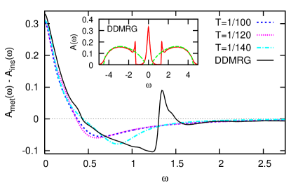
Figure 5: (Color online) Inset: DDMRG spectra of coexisting metallic and insulating phases at $U=5.2$, reproduced from Karski05 . Main panel: difference spectra from multigrid HF-QMC (broken lines) and DDMRG Karski05 (solid line).

this study finds sharp features at the inner edges of the Hubbard bands in the strongly correlated metallic phase (solid lines), which are separated from the quasiparticle peak by quite broad pseudo gaps; in contrast, the Hubbard bands appear rather featureless in the insulating phase (dashed lines) for the same interaction $U=5.2$, with inner edges that are shifted to much smaller frequencies. Obviously this behavior, which has been interpreted in terms of collective magnetic excitations in the metal Karski05 , should be verified. One may also ask whether it extends to finite temperatures, i.e., governs the spectral weight transfer at the Mott transition, which, for $U=5.2$, occurs at $T\approx 1/100$.

Estimates of the spectral weight transfer, the difference of metallic and insulating spectra, are shown in the main panel of Fig. 5. At this scale, the DDMRG data (solid line) clearly resolves the features discussed above, in particular the Hubbard subpeak at $|\omega|\approx 1.3$. The corresponding multigrid HF-QMC results (broken lines) have been obtained, for minimal bias, via Padé analytic continuation of Matsubara difference Green functions. They are much smoother even at very low $T$: apart from the quasiparticle peak, with a reduced weight, only a shallow negative region at $0.4\lesssim\omega\lesssim 1.5$ is visible, which is evidence against the existence of subpeaks. We obviously cannot exclude that this smoothness is, at least partially, an artifact of the ill-conditioned analytic continuation; it is also not clear whether the change of shape at the lowest temperature $T=1/140$, with a closer approach of the DDMRG line shape, is significant. In contrast, the QMC difference Green functions shown in Fig. 6 as broken lines (basis for the spectral data of Fig. 5) are precise within linewidth. In the low-$\tau$ regime that we are focusing on, even the extrapolation to $T=0$ is reliable (see inset of Fig. 6). However, the transformed DDMRG data (thin solid line in main panel) deviates markedly from this QMC ground state result (thick solid line, with a precision of about linewidth): the DDMRG overestimates the differences between metal and insulator, in this measure, by about $10\%$, with an even larger discrepancy compared to the finite-temperature result at $T=1/100$, where the metal-insulator transition takes place. We conclude that the DDMRG does not capture the spectral-weight transfer at the Mott transition quantitatively correctly; possible explanations include the bias towards metallic/insulating solutions for odd/even chains in the DMRG calculation and, in particular, the deconvolution technique. In terms of spectra, a large part of the DDMRG error can be traced back to its overestimation of the quasiparticle peak (since the QMC data of Fig. 5 is particularly reliable in this range); similar mechanisms might have generated the Hubbard-band subpeaks.

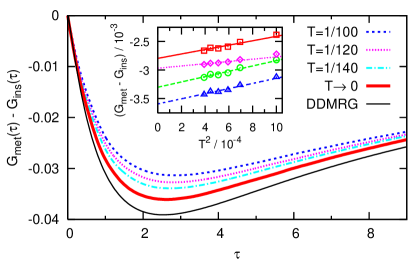
Figure 6: (Color online) Difference Green functions from QMC at finite $T$ (dashed, dotted lines) and extrapolated to $T=0$ (thick solid line) versus DDMRG data (thin line). Inset: extrapolation $T\to 0$ for $\tau=1,6,1.5,2.5$ (top to bottom).

Discussion – We have formulated a new algorithm for solving Hubbard-type models within DMFT, based on a multigrid implementation of the HF-QMC method with internal Green function extrapolation. This technique directly yields numerically exact results even at very low temperatures, similarly to recently developed continuous-time QMC methods. However, our algorithm retains the advantages of HF-QMC, i.e., generates Green functions with minimal fluctuations, now at about halved temperatures for similar precision and effort. The method extends to the general multi-band case, with enormous potential, e.g., in the context of ab initio LDA+DMFT calculations. While it is too early to judge which of the three (quasi) continuous-time methods will ultimately prevail, our multigrid method clearly supersedes conventional HF-QMC for most applications.

Using this method, we have found inconsistencies in the DDMRG scenario of the spectral weight transfer at the Mott transition. A definite judgement whether the DDMRG results are, at least, qualitatively correct, will require additional computing ressources and detailed analyses of analytical continuation procedures.

Stimulating discussions with P.G.J. van Dongen and support by the DFG within the Collaborative Research Centre SFB/TR 49 are gratefully acknowledged.

References

- (1) See G. Kotliar and D. Vollhardt, Physics Today 57, 53 (2004) and references therein.
- (2) See R. Martin, Electronic structure, Cambridge University Press (2004) and references therein.
- (3) A. Georges, G. Kotliar, W. Krauth, and M. Rozenberg, Rev. Mod. Phys. 68, 13 (1996).
- (4) J. E. Hirsch and R. M. Fye, Phys. Rev. Lett. 56, 2521 (1986); M. Jarrell, Phys. Rev. Lett. 69, 168 (1992).
- (5) N. Blümer and E. Kalinowski, Phys. Rev. B, 71, 195102 (2005); Physica B 359, 648 (2005).
- (6) N. Blümer, Phys. Rev. B 76, 205120 (2007).
- (7) A.N. Rubtsov, V.V. Savkin, and A.I. Lichtenstein, Phys. Rev. B 72, 035122 (2005).
- (8) P. Werner, A. Comanac, L. de Medici, M. Troyer, and A. J. Millis, Phys. Rev. Lett. 97, 076405 (2006).
- (9) M. Karski, C. Raas, and G. S. Uhrig, Phys. Rev. B 72, 113110 (2005).
- (10) N. Blümer, arXiv:0712.1290v1 (unpublished).
- (11) E.g.: 100–400 time slices in HF-QMC, 1000 Matsubara frequencies for state variables, 10000 interpolated time slices, and 40000 Matsubaras for the reference model.
- (12) N. Blümer, in preparation.
- (13) G. Kotliar, E. Lange, and M. J. Rozenberg, Phys. Rev. Lett. 84, 5180 (2000).
- (14) We have verified that the assumed extrapolation law remains accurate at least up to , when is increased from 3 to about 8.