Non-perturbative QED Model with Dressed States to Tackle HHG in Ultrashort Intense Laser Pulses

Abstract

A generalization of non-perturbative QED model for high harmonic generation is developed for the multi-mode optical field case. By introducing classical-field-dressed quantized Volkov states analytically, a formula to calculate HHG for hydrogen-like atom in ultrashort intense laser pulse is obtained, which has a simple intuitive interpretation. The dressed state QED model indicates a new perspective to understand HHG, for example, the presence of the weak even-order harmonic photons, which has been verified by both theoretical analysis and numerical computation. Long wavelength approximation and strong field approximation are involved in the development of the formalism.

High order harmonic generation (HHG), that atoms subjected to an intense laser field emit more than a hundredth-order harmonic photons, is the highest nonlinear optical phenomenon ever observedexperiments . It has triggered a series of experimental and theoretical researches. HHG not only offers an approach to the table-top source for coherent XUV and soft x-ray generationxray , but also to attosecond light pulsesfiratto . The latter has been used to probe ultrafast atomic and molecular dynamics, eg. atom ionization and correlation, molecule rearrangement, molecule dissociation and so onionization .

HHG has been widely understood as a three-step process — the ionization, propagation and recombination. Calculations have been carried out by direct numerical integration of the time-dependent Schrödinger equation, using base expansion or grid methodsnolinearintegral . In addition, various theoretical models concerning essential physical processes in intense laser field and less computer intensive are widely studied. For example, the KFR model for the scatteringKFR , the ADK model for the ionizationADK , the Lewenstein model for HHGSFA , and so on. These models are based on the classical treatment of the laser field. In these semiclassical models, the HHG spectrum is obtained by the Fourier transform of the time-dependent electric dipole, or the dipole acceleration.

On the other hand, the observed discrete HHG spectrum indicates that it is an optical-conversion process in which $q$ pump photons are combined to produce a single, harmonic photonjgaoprl . This picture favors the QED approach which treats the photon field as a quantized field. It is capable of presenting a clearer picture of how the photons are being absorbed and emitted, and how the energy and momentum transfer between the optical field and the atom. A non-perturbative QED scattering theory of single-mode case has been developed for HHGguo . It provides a new perspective to understand HHG, for example, rather than by extracting HHG spectrum from the time-dependent atomic wavepacket, it self-contains harmonic photon emitting in the theory. Similar phenomena at much higher intensities can be calculated on its framework. It has successfully reproduced the salient characteristics of experimental spectra and revealed the connection between high harmonic generation and above threshold ionizationguo ; jgaoprl ; korean .

The essential part of QED model for HHG in a intense laser field is the transition matrix elementguo ; jgaoprl ; korean

$$T_{fi}=\sum_{\mu}\langle\Psi_{f}|V^{{}^{\prime}}|\Psi_{\mu}\rangle\langle\Psi_{\mu}|V|\Psi_{i}\rangle\delta_{\mu}\;,$$ (1)

where $\Psi_{i}$ is the initial state of the atom-photon system, $\Psi_{f}$ is the final state with a harmonic photon, $\Psi_{\mu}$ is a quantized-field Volkov state, and $V\,(V^{{}^{\prime}})$ is the interaction potential. The symbol $\delta_{\mu}$ represents energy conservation condition in the non-relativistic case. Eq. (1) gives a physical picture that the atom in an intense optical field can simultaneously absorb more than one photon to transit to the quantized-field Volkov states, and finally emit a harmonic photon to transit to the final state.

The quantized-field Volkov states are the pivotal part of the QED approach. Classical Volkov statesvolkov , which are the solutions of time-dependent Schrödinger equation for a free electron in a classical electromagnetic field, are incorporated in the KFR theory to form a non-perturbative scattering framework for multiphoton ionization (MPI). Later, Guo, Åberg and Drake obtained analytical solutions for an free electron in an intense quantized optical fieldAberg ; Drake —the quantized-field Volkov states, based on which the QED calculation for HHG is developed.

Most of the calculations for HHG in QED have been carried out by assuming the fundamental laser field to be single-mode guo ; jgaoprl ; korean . The formal scattering theory, which takes the interaction time as infinity, is always used. This is a good approximation to many experiments in which the laser pulse’s duration is dozens of optical cycles long so that the laser field can be considered as single-mode. However, it still limits the usage of the method in certain ways. For example, the effect of the laser pulse’s shape cannot be studied, the calculated HHG spectrum only contains the photon frequencies which are multiples of the fundamental frequency, and ultrafast atom-laser interactions are hard to describe.

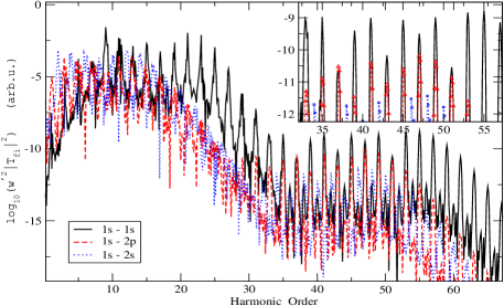
Figure 1: HHG spectrum of H atom for the laser parameters: $\lambda=0.8\mu m$, peak intensity $I=3.5\times 10^{14}W/cm^{2}$, gaussian pulse shape with $FWHM=16fs$. The solid line is $1s-Volkov\,state-1s$ transition, the dash line is $1s-Volkov\,state-2p$ transition, and the dot line is $1s-Volkov\,state-2s$ transition. The inset shows a part of the spectrum from harmonic order 33 to 55.

In the present study, we improve the QED model to the multi-mode case by taking the Born-Oppemheimer approximation, that the photon mode is a far more rapidly varying degree of freedom than the electron, so the stimulated electron-photon interactions dress the atomic electron. Therefore, in the multi-mode case, the interaction is between the photons and the photon-cloud-dressed electron, instead of the naked electron as in the previous models. Similar idea has been used in studying laser-assisted bremsstrahlung in highly intense laser fieldkeitel .

Two key techniques are used in our theory. Firstly, we treat the strongest mode of the laser field as the quantized mode, which has the same optical cycle as the laser pulse. By deriving the classical-field-dressed quantized Volkov states, the effects of all the other modes are incorporated as a classical distortion field which dresses the quantized Volkov state. Secondly, we make use of the Fourier transform of the evolution operator, instead of the time-independent formal scattering formalism. This allows us to include time in the theory. The inverse operators are transformed to computable integrals by the equations we derive.

We differ from the previous studiesguo ; jgaoprl ; korean by using coherent states instead of Fock states to describe the laser field. Coherent state $|\alpha_{1}\alpha_{2}\cdots\rangle$, where $|\alpha_{k}\rangle=\exp^{-\frac{|\alpha_{k}|^{2}}{2}}\sum\limits_{n=0}\limits^{\infty}{\frac{\alpha_{k}^{n}}{\sqrt{n!}}|n\rangle}$ is the eigenstate of the annihilation operator $\hat{a}_{k}$ with $\hat{a}_{k}|\alpha_{k}\rangle=\alpha_{k}|\alpha_{k}\rangle$, is a better approximation to the real laser fieldcoherent : $\langle\alpha_{1}(t)\alpha_{2}(t)\cdots|\mathbf{\hat{A}}|\alpha_{1}(t)\alpha_{2}(t)\cdots\rangle=\sum{\mathbf{A}_{i}(t)}=\mathbf{A}(t)$, where $\mathbf{A}(t)=\hat{\epsilon}A(t)$ is the electromagnetic field vector. In this treatment, the absolute value and the phase of $\alpha_{k}$ are in accordance with the amplitude and the phase of the kth mode of the laser field. Therefore it provides a way to characterize the time-dependence of the laser pulse by $\alpha_{k}=\frac{1}{T}\int\limits_{0}\limits^{T}d\tau e^{iw_{k}\tau}A(\tau).$ The long wavelength limit is taken in the present scheme. Walser et al.multipole have considered the multipole contributions to HHG, and found such effects be small below an intensity of about $10^{17}W/cm^{2}$.

In the non-relativistic case, the total hamiltonian of a hydrogen-like atom in the optical field is $\hat{H}=\hat{H_{0}}+\hat{V}_{T}$, where $\hat{H_{0}}=\frac{1}{2m}\mathbf{\hat{p}}^{2}+\sum{\omega_{k}(\hat{N}_{k}+\frac{1}{2})}+\omega^{{}^{\prime}}(\hat{N}^{{}^{\prime}}+\frac{1}{2})+\hat{U}$ is the noninteraction part of the Hamiltonian. $\hat{U}$ is the atomic binding potential; $\hat{N^{{}^{\prime}}}$ and $\hat{N}_{k}$ are photon number operators of harmonic mode with frequency $\omega^{{}^{\prime}}$ and the kth laser mode with frequency $\omega_{k}$, respectively. $\hat{V}_{T}$ is the electron-photon interaction term $\hat{V}_{T}=-\frac{e}{m}\mathbf{\hat{p}}\cdot\mathbf{\hat{A}}+\frac{e^{2}}{2m}\mathbf{\hat{A}}^{2}$. Due to the weakness of the harmonic mode, $\hat{V}_{T}$ can be divided as $\hat{V}_{T}=\hat{V}+\hat{V}^{{}^{\prime}}$

$$\hat{V}=-\frac{e}{m}(\mathbf{\hat{A}}_{c}+\mathbf{\hat{A}}_{s})\cdot\mathbf{\hat{p}}+\frac{e^{2}}{2m}(\mathbf{\hat{A}}_{c}+{\mathbf{\hat{A}}_{s}})^{2}\;,$$ (2)

$$\hat{V}^{{}^{\prime}}=-\frac{e}{m}\mathbf{\hat{A}}^{{}^{\prime}}\cdot\mathbf{\hat{p}}+\frac{e^{2}}{m}\mathbf{\hat{A}}^{{}^{\prime}}\cdot(\mathbf{\hat{A}}_{c}+\mathbf{\hat{A}}_{s})\;.$$ (3)

For simplicity, we denote $\mathbf{\hat{A}}^{{}^{\prime}}$ as the harmonic mode, $\mathbf{\hat{A}}_{c}$ as the quantized laser mode, and $\mathbf{\hat{A}}_{s}=\sum\limits_{s\neq c}\mathbf{\hat{A}}_{s}$ as all the other laser modes, so $\mathbf{\hat{A}}=\mathbf{\hat{A}}_{c}+\mathbf{\hat{A}}_{s}+\mathbf{\hat{A}}^{{}^{\prime}}$. In general, $\mathbf{\hat{A}}_{u}=g_{u}(\hat{\epsilon}_{u}\hat{a}_{u}e^{i\mathbf{k}_{u}\cdot\mathbf{r}}+c.c.)$, where the polarization vector $\hat{\epsilon}$ is given by $\hat{\epsilon}=cos(\xi/2)\hat{\epsilon}_{x}+isin(\xi/2)\hat{\epsilon}_{y}$, where $\xi$ is a measure of the degree of ellipticity, then $\xi=0$ and $\pi/2$ corresponding to linear and circular polarization, respectively guo . The driving optical field in our calculation is linearly polarized.

The non-perturbative approach for HHG is based on the fourier transform of the evolution operator $\hat{U}(t,t^{{}^{\prime}})$ evolution

$$\hat{U}(t,t^{{}^{\prime}})= -\frac{1}{2\pi i}\int_{-\infty}^{+\infty}dz\frac{e^{-iz\tau}}{z-\hat{H}+i\epsilon}\Theta(\tau)$$

$$+\frac{1}{2\pi i}\int_{-\infty}^{+\infty}dz\frac{e^{-iz\tau}}{z-\hat{H}-i\epsilon}\Theta(-\tau)\;,$$ (4)

where $\tau=t-t^{{}^{\prime}}$, $\Theta(\tau)=1$ when $\tau\geq 0$ and $\Theta(\tau)=0$ when $\tau<0$ ; $\epsilon\rightarrow 0_{+}$. The operator can be expanded, giving the matrix element for the harmonic generation process as guo ; jgaoprl ; korean

$$T_{fi} =\langle\Psi_{f}(T)|\hat{U}(T,0)|\Psi_{i}(0)\rangle$$

$$=-\frac{1}{2\pi i}\int_{-\infty}^{+\infty}dze^{-izT}e^{i(E^{a}_{f}+\frac{3}{2}w^{{}^{\prime}})T}\times\langle\Phi_{f},\alpha_{f}(T),1^{{}^{\prime}}|$$

$$\times\frac{1}{z-\hat{H}_{0}+i\epsilon}V^{{}^{\prime}}\frac{1}{z-\hat{H}+i\epsilon}V\frac{1}{z-\hat{H}_{0}+i\epsilon}$$

$$\times|\Phi_{i},\alpha_{i}(0),0^{{}^{\prime}}\rangle\;,$$ (5)

where the system’s initial and final states are decoupled states of the electron and the laser field, and the laser pulse is confined to the interval $[0,T]$. $\Phi_{i,f}$ is the wave function of the atomic electron with binding energy $E^{a}_{i,f}$; $|n^{{}^{\prime}}\rangle$, with $n=0,1$, is the harmonic photon Fock state, and $|\alpha_{i,f}(t)\rangle=e^{-i\frac{w_{1}+w_{2}+\cdots}{2}t}|\alpha^{1}_{i,f}e^{-iw_{1}t},\alpha^{2}_{i,f}e^{-iw_{2}t},\cdots\rangle$ is the coherent laser state .

If $\Phi$ is the eigenstate of the atomic hamiltonian and $\hat{H}_{0}$ is the noninteraction hamiltonian, we get the relations

$$\frac{1}{z-\hat{H}_{0}+i\epsilon}|\Phi(t_{0})\alpha(t_{0})\rangle$$

$$= -i\int^{+\infty}_{-\infty}dte^{izt}|\Phi(t+t_{0})\alpha(t+t_{0})\rangle\Theta(t)$$

$$= -i\int^{+\infty}_{0}dte^{izt}|\Phi(t+t_{0})\alpha(t+t_{0})\rangle\;,$$

$$\langle\Phi(t_{0})\alpha(t_{0})|\frac{1}{z-\hat{H}_{0}+i\epsilon}$$

$$= -i\int^{+\infty}_{-\infty}dte^{-izt}\langle\Phi(t+t_{0})\alpha(t+t_{0})|\Theta(-t)$$

$$= -i\int^{0}_{-\infty}dte^{-izt}\langle\Phi(t+t_{0})\alpha(t+t_{0})|\;.$$ (7)

Then the transition matrix $T_{fi}$ becomes

$$T_{fi} =\frac{1}{2\pi i}\int_{-\infty}^{+\infty}dz\int^{0}_{-\infty}dt_{1}\int^{+\infty}_{0}dt_{2}e^{-i[z-(E^{a}_{f}+\frac{3}{2}w^{{}^{\prime}})](T+t_{1})}$$

$$\times\langle\Phi_{f},\alpha_{f}(T+t_{1}),1^{{}^{\prime}}|V^{{}^{\prime}}\frac{1}{z-\hat{H}+i\epsilon}V|\Phi_{i},\alpha_{i}(t_{2}),0^{{}^{\prime}}\rangle$$

$$\times e^{-iE^{a}_{i}t_{2}}\;.$$ (8)

Therefore, the two inverse operators have been transformed into computable integrals.

To apply this strategy further to tackle Eq. (Non-perturbative QED Model with Dressed States to Tackle HHG in Ultrashort Intense Laser Pulses), we need the knowledge of the eigenstates of $\hat{H}$. Due to the weakness of $\hat{V^{{}^{\prime}}}$ and the strong field approximation(SFA), the binding potential $\hat{U}$ can be neglected for continuum electron statesSFA , hence only the leading term of the inverse operator $\frac{1}{z-\hat{H}+i\epsilon}$ has to be kept, thus enabling $\hat{U}$ and $\hat{V}^{{}^{\prime}}$ in the denominator in Eq. (Non-perturbative QED Model with Dressed States to Tackle HHG in Ultrashort Intense Laser Pulses) to be droppedguo .

In the one-mode case, the eigenstates of such a Hamiltonian are the quantized-field Volkov statesAberg : $\Psi_{pn}=V^{-1/2}_{e}\sum\limits_{j=-n}\limits^{\infty}e^{i[\mathbf{p}+(u_{p}-j)\mathbf{k}]\cdot\mathbf{r}}\times\mathcal{J}_{j}(\zeta,\eta,\phi_{\xi})^{*}\times e^{-ij\phi_{\xi}}|n+j\rangle$ with corresponding energy eigenvalues $E_{pn}=\frac{\mathbf{p}^{2}}{2m}+(n+1/2+u_{p})w$. $u_{p}=\frac{e^{2}\Lambda^{2}}{mw}$ is the ponderomotive energy in units of the photon energy of the laser, where $\Lambda$, as the limit of $g\sqrt{n}(g\rightarrow 0,\sqrt{n}\rightarrow\infty)$, is the half amplitude of the classical field; $\zeta=\frac{2e\Lambda}{mw}|\mathbf{p}\cdot\hat{\epsilon}|$ , $\eta=\frac{1}{2}u_{p}cos\xi$ and $\phi_{\xi}=\arctan(\frac{p_{y}}{p_{x}}\tan\frac{\xi}{2})$. The generalized Bessel function $\mathcal{J}_{j}(\zeta,\eta,\phi_{\xi})$ is $\mathcal{J}_{j}(\zeta,\eta,\phi_{\xi})=\sum\limits_{m=-\infty}^{\infty}J_{-j-2m}(\zeta)J_{m}(\eta)e^{i2m\phi_{\xi}}$.

In the multi-mode case, with one specified quantized mode ($A_{c}$), we obtain the classical-field-dressed quantized-field Volkov states

$$\widetilde{\Psi}^{c}_{pn}(t) =e^{ie\sum\mathbf{A}_{s}(t)\cdot\mathbf{r}}|\Psi^{c}_{pn}(t)\rangle|\alpha^{s}(t)\rangle,$$

$$=V_{e}^{-1/2}e^{ie\sum\mathbf{A}_{s}(t)\cdot\mathbf{r}}|\alpha^{s}(t)\rangle\sum\limits_{j=-n_{c}}\limits^{\infty}e^{i[\mathbf{p}+(u^{c}_{p}-j)\mathbf{k_{c}}]\cdot\mathbf{r}}$$

$$\times\mathcal{J}_{j}(\zeta_{c},\eta_{c},\phi^{c}_{\xi})^{*}e^{-ij\phi^{c}_{\xi}}|n_{c}+j\rangle e^{-iE_{pn_{c}}t}\;.$$ (9)

As before, the script $s$ represents all the other modes in the laser field except the mode distinguished by $c$. In the large-photon-number limit, where $a^{+}|\alpha\rangle=\alpha^{*}|\alpha\rangle$ for $|\alpha|\rightarrow\infty$, $\widetilde{\Psi}^{c}_{pn}$ has the property

$$(\frac{1}{2m}(\mathbf{\hat{p}}-e\mathbf{\hat{A}})^{2}+\sum{\omega_{k}(\hat{N}_{k}+\frac{1}{2})})\widetilde{\Psi}^{c}_{pn}$$

$$= (E^{c}_{pn}+E_{s})\widetilde{\Psi}^{c}_{pn}$$ (10)

Where $E_{s}=\sum w_{s}|\alpha_{s}|^{2}$. Eq. (Non-perturbative QED Model with Dressed States to Tackle HHG in Ultrashort Intense Laser Pulses) verifies that the classical-field-dressed quantized-field Volkov state is the approximate eigenstate of the electron-laser subsystem in the multi-mode field. Therefore, a relation similar to Eq. (Non-perturbative QED Model with Dressed States to Tackle HHG in Ultrashort Intense Laser Pulses) can be obtained

$$\frac{1}{z-H+i\epsilon}e^{ie\sum\mathbf{A}^{s}(t_{0})\cdot\mathbf{r}}|\Psi^{c}_{pn}(t_{0})\rangle|\alpha^{s}(t_{0})\rangle$$

$$= -i\int^{+\infty}_{0}dte^{izt}e^{ie\sum\mathbf{A}^{s}(t_{0}+t)\cdot\mathbf{r}}$$

$$\times|\Psi^{c}_{pn}(t_{0}+t)\rangle|\alpha^{s}(t_{0}+t)\rangle\;.$$ (11)

Combining Eq. (Non-perturbative QED Model with Dressed States to Tackle HHG in Ultrashort Intense Laser Pulses) and (Non-perturbative QED Model with Dressed States to Tackle HHG in Ultrashort Intense Laser Pulses), and after the integration of the energy $z$, we get

$$T_{fi}= \frac{1}{2\pi}\sum\limits_{pn}\int^{T}_{0}d\tau_{1}\int^{T}_{\tau_{1}}d\tau_{2}\langle\Phi_{f},\alpha^{c}_{f},1^{{}^{\prime}}|V^{{}^{\prime}}(\tau_{2})e^{ie\sum\mathbf{A}^{s}(\tau_{2})\cdot\mathbf{r}}|\Psi^{c}_{pn},0^{{}^{\prime}}\rangle$$

$$\times e^{i(E^{a}+\omega^{{}^{\prime}}_{f}-E^{c}_{pn})\tau_{2}}e^{-i(E^{a}_{i}-E^{c}_{pn})\tau_{1}}\langle\Psi^{c}_{pn},0^{{}^{\prime}}|e^{-ie\sum\mathbf{A}^{s}(\tau_{1})\cdot\mathbf{r}}V(\tau_{1})|\Phi_{i},\alpha^{c}_{i},0^{{}^{\prime}}\rangle\;,$$ (12)

where $V(\tau_{1})=\frac{e^{2}}{2m}\mathbf{A}^{2}(\tau_{1})-\frac{e}{m}\mathbf{A}(\tau_{1})\cdot(\mathbf{p}+e\sum\mathbf{A}^{s}(\tau_{1})+(u^{c}_{p}-j)\mathbf{k}_{c})$ and $V^{\prime}(\tau_{2})=\frac{e^{2}}{2m}g^{\prime}\hat{\epsilon}^{{}^{\prime}*}\cdot\mathbf{A}(\tau_{2})-\frac{e}{m}g^{\prime}\hat{\epsilon}^{{}^{\prime}*}\cdot(\mathbf{p}+e\sum\mathbf{A}^{s}(\tau_{2})+(u^{c}_{p}-j)\mathbf{k}_{c}$.

Eq. (Non-perturbative QED Model with Dressed States to Tackle HHG in Ultrashort Intense Laser Pulses) indicates that the probability amplitude of emitting a harmonic photon is the sum of the probability amplitudes of all the individual events in which the electron is ionized at some time and recombines with the nucleus to emit the photon at a later time. The picture is intuitive, but is not trivial for these probabilities add up in an interference way.

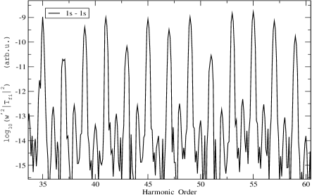
Figure 2: One Part of HHG spectrum of H atom for the same laser parameters as in Fig. (1). It only shows HHG from $1s-Volkov\,state-1s$ transition.

HHG of H atom in an intense ultrashort laser pulse has been calculated as a numerical example. The laser parameters are: $\lambda=0.8\mu m$, peak intensity $I=3.5\times 10^{14}W/cm^{2}$, gaussian pulse shape with $FWHM=16fs$, that is approximately 6 optical cycles. The atom is assumed to be initially in the ground state. Different lines in Fig (1) represent different final state cases, here the $1s$, $2p$, $2s$ states respectively. It shows that, among the three transitions considered here, $1s-Volkov\,states-1s$ transition dominates the harmonic photon generation. The contributions from other transitions are about $10^{-1\sim-2}$ smaller in the plateau. It demonstrates that the SFA, where only the recombination to the ground state is taken into account, is a good approximation in this case. This QED model can then be used to complement other models by indicating what bound states should be included in the approximation.

The fine structures of HHG in Fig (2) show the generation of even-order harmonic photons. The presence of even harmonics can be explained as the contribution of $\frac{e^{2}}{2m}\mathbf{\hat{A}}^{2}$, which can not be considered as a perturbation as in the weak light field case. Transition through $-\frac{e}{m}\mathbf{\hat{p}}\cdot\mathbf{\hat{A}}$ changes the atomic state’s parity, while transition through $\frac{e^{2}}{2m}\mathbf{\hat{A}}^{2}$ maintains it. Therefore, the argument for the absence of even harmonics, that is the selection rule for the dipole transition, does not hold here. In this laser parameter condition, the intensity of the even harmonics is much weaker than the odd ones, with a factor $10^{-4}$. This is in accordance with the experiments where only odd harmonics are observed. However, in the semi-classical model, or numerically solving TDSE, the information of even harmonics is often buried by the numerical noise or more importantly, by other weaker transitions, like $1s-Volkov\,states-2s$ and $1s-Volkov\,states-2p$ shown here.

In conclusion, a generalization of non-perturbative QED model for HHG has been developed to the multi-mode case. In our QED model, HHG produced by ultrashort laser pulse can be calculated for hydrogen-like atoms. A numerical example has been calculated for H atom in intense ultrashort laser pulse and it reveals a clear evidence of even harmonics generation.

References

• (1) M. Ferray et al., J. Phys. B 21, L31(1988); A. McPherson et al., J. Opt. Soc. Am. B 4, 595 (1987)
• (2) Z. H. Chang et al., Phys. Rev. Lett. 79, 2967 (1997)
• (3) A. Scrinzi, M. Yu Ivanov, R. Kienberger and D. M. Villeneuve, J. Phys. B 39, R1 (2006); T. Pfeifer, C. Spielmann and G. Gerber, Rep. Prog. Phys. 69, 443 (2006)
• (4) R. Velotta et al., Phys. Rev. Lett. 87, 183901 (2001). J. Itatani et al., Phys. Rev. Lett. 94, 123902 (2005); M. Lein, Phys. Rev. Lett. 94, 053004 (2005); S. Baker et al., Science 312, 424 (2006)
• (5) M. Protopapas, C. H. Keitel and P. L. Knight, Rep. Prog. Phys. 60, 389 (1997)
• (6) M. V. Ammosov, N. B. Delone, V. P. Krainov, Sov.Phys.-JETP 64, 1191 (1986); P. B. Corkum, Phys. Rev. Lett. 71, 1994 (1993)
• (7) L. V. Keldysh, Zh. Eksp. Teor. Fiz. 47, 1945 (1964); F. H. M. Faisal. J. Phys. B 6, L89 (1973); H. R. Reiss, Phys. Rev. A 22, 1786 (1980)
• (8) D. M. Volkov, Z. Phys. 94, 250 (1935)
• (9) M. Lewenstein et al., Phys. Rev. A 49, 2117 (1994)
• (10) L. H. Gao et al., Phys. Rev. A 61, 063407 (2000)
• (11) J. Gao, F. Shen, and J. G. Eden, Phys. Rev. Lett. 81, 1833 (1998)
• (12) J. Gao, F. Shen, and J. G. Eden, Phys. Rev. A 61, 043812 (2000)
• (13) Claude Cohen-Tannoudji, Jacques Dupont-Roc, Gibert Grynberg, Atom-Photon Interactions (Basic Process and Applications), (John Wiley $\&$ Sons, Inc., 1992)
• (14) E. LΓΆtstedt, U. D. Jentschura and C. H. Keitel, Phys. Rev. Lett. 98, 043002 (2007)
• (15) D. S. Guo and G. W. F. Drake, J. Phys. A 25, 3383 (1992)
• (16) D. S. Guo and G. W. F. Drake, J. Phys. A 25, 5377 (1992)
• (17) Leonard Mandel and Emily Wolf, Optical Coherence and Quantum Optics (Cambridge, 1995); Marlan O.Scully and M.Suhail Zubairy(Cambridge, 1997)
• (18) M. W. Walser, C. H. Keitel, A. Scrinzi and T. Brabec, Phys. Rev. Lett. 85, 5082 (2000)