BF Eridani: a cataclysmic variable with a massive white dwarf and an evolved secondary

Abstract

We present high- and medium-resolution spectroscopic observations of the cataclysmic variable BF Eri during its low and bright states. The orbital period of this system was found to be 0.270881(3) days. The secondary star is clearly visible in the spectra through absorption lines of the neutral metals Mg i, Fe i and Ca i. Its spectral type was found to be K3$\pm$0.5. A radial velocity study of the secondary yielded a semi-amplitude of $K_{2}=182.5\pm 0.9$ km s^-1. The radial velocity semiamplitude of the white dwarf was found to be $K_{1}=74\pm 3$ km s^-1 from the motion of the wings of the H$\alpha$ and H$\beta$ emission lines. From these parameters we have obtained that the secondary in BF Eri is an evolved star with a mass of 0.50–0.59 $M_{\odot}$, whose size is about 30 per cent larger than a zero-age main-sequence single-star of the same mass. We also show that BF Eri contains a massive white dwarf ($M_{1}\geq 1.23M_{\odot}$), allowing us to consider the system as a SN Ia progenitor. BF Eri also shows a high $\gamma$-velocity ($\gamma\ =-94$ km s^-1) and substantial proper motion. With our estimation of the distance to the system ($d\approx 700\pm 200$ pc), this corresponds to a space velocity of $\sim$350 km s^-1 with respect to the dynamical local standard of rest. The cumulative effect of repeated nova eruptions with asymmetric envelope ejection might explain the high space velocity of the system. We analyze the outburst behaviour of BF Eri and question the current classification of the system as a dwarf nova. We propose that BF Eri might be an old nova exhibiting “stunted” outbursts.

1 Introduction

Cataclysmic Variables (CVs) are close interacting binaries that contain a white dwarf (WD) accreting material from a companion, usually a late main-sequence star. CVs are very active photometrically, exhibiting variability on time scales from seconds to centuries (see review by Warner 1995). Dwarf novae (DNs) are an important subset of CVs. Observable features that distinguish DN from other CVs such as nova-like variables (NLs) are the recurrent outbursts of 2–6 mag that occur on timescales of days to years. In this paper we concentrate on BF Eridani, a little-studied dwarf nova candidate.

BF Eri was discovered and first classified as a slowly varying variable star by Hanley & Shapley (1940). During the following half a century no observations of the star were reported. As a consequence, the specific nature of the star remained unknown. The identification of the Einstein survey source 1ES 0437-046 with BF Eri (Elvis et al., 1992) and optical spectroscopy by Schachter et al. (1996) eventually led to its correct identification as a CV. Later, the ROSAT identification of the Einstein source confirmed the classification of BF Eri as a CV of an unknown type (Chisholm et al., 1999).

Table 1: Log of observations of BF Eri

Set	Date	HJD Start	Instrument	$\Delta\lambda$a	$\lambda$ range	Exp.Time	Number	Duration
		2450000+		(Å)	(Å)	(sec)	of exps.	(hours)
2005-N1	2005-Oct-30	3673.982	B&Chb	6.0	3680–6770	300	16	1.44
2005-N2	2005-Oct-31	3674.821	B&Ch	6.0	6025–8000	300	40	3.50
2005-N3	2005-Nov-01	3675.821	B&Ch	2.1	6145–7225	300	58	5.25
2006-Nov
2006-N1	2006-Nov-22	4061.884	Echelle	0.234	3915–7105	1200	9	3.13
2006-N2	2006-Nov-23	4062.728	Echelle	0.234	3915–7105	1200	17	6.81
2006-N3	2006-Nov-24	4063.710	Echelle	0.234	3915–7105	1200	19	7.08
2006-N4	2006-Nov-25	4064.684	Echelle	0.234	3915–7105	1200	3	0.70
		4064.879	Echelle	0.234	3915–7105	1200	3	0.70
2006-N5	2006-Nov-26	4065.698	Echelle	0.234	3915–7105	1200	20	7.26
2006-N6	2006-Nov-27	4066.689	Echelle	0.234	3915–7105	1200	14	4.78
2006-Dec
	2006-Dec-13	4082.840	Echelle	0.234	3915–7105	1200	2	0.35
	2006-Dec-14	4083.850	Echelle	0.234	3915–7105	1200	2	0.35
	2006-Dec-15	4084.808	Echelle	0.234	3915–7105	1200	2	0.36

a – $\Delta\lambda$ is the FWHM spectral resolution

b – B&Ch - Boller & Chivens spectrograph

The long term light curve was first analysed by Watanabe (1999) who detected two outbursts and concluded that BF Eri is a DN with a recurrence period of 40–50 days and the observed magnitude range between 13.2 and fainter than 14.7 mag. Kato (1999) and Kato & Uemura (2000) confirmed this classification but mentioned the low amplitude of its outbursts and the difference in the outburst activity between seasons as the amplitudes of outbursts were remarkably different – 1.0 mag and 1.6 mag. Kato (1999) was unable to detect any orbital variability.

Prior to the beginning of this work there was no other study of the system in the literature. This motivated us to perform time-resolved spectroscopy of BF Eri in order to study its properties in more detail. In this paper we present and discuss the first high- and medium-resolution spectroscopic observations of BF Eri during its low and bright states in 2005 and 2006. In Section 2 we describe our observations and data reduction. The data analysis and the results are presented in Section 3. Here we find the orbital period, measure the radial velocities of the WD and the secondary star, and determine the spectral type of the secondary and its rotational velocity. In Section 4 we discuss the results of Doppler tomography of the emission lines from BF Eri. The system parameters are obtained in Section 5, while a discussion and a summary are given in Sections 6 and 7, respectively.

Figure 1: The average spectra of BF Eri from the 2005 set, uncorrected for orbital motion. The lower spectrum is combined from the 2005-N1 and 2005-N2 sets while the inset spectrum is an average of all spectra from the 2005-N3 set.

2 Observations and Data reduction

The spectra presented here were obtained at the Observatorio Astronomico Nacional (OAN SPM) in Mexico on the 2.1 m telescope. The first observations, in 2005, were conducted with the Boller & Chivens spectrograph, equipped with a 24 $\mu$m ($1024\times 1024$) SITe CCD. Observations were made during three consecutive nights of October 30–31 – November 1 in the wavelength range of 3680–6770 Å, 6025–8000 Å and 6145–7225 Å respectively. Spectra were obtained in the first order of 400 line/mm (for the first two nights) and 1200 line/mm (for the third night) gratings with corresponding spectral resolutions of around 6.0 Å and 2.1 Å respectively. A total of 114 spectra were obtained with 300 s individual exposures, half of them on the third night. Cu-He-Ne-Ar lamp exposures were taken before and after the observations of the target for wavelength calibrations, and the standard spectrophotometric stars Feige110, HR3454 and G191-B2B (Oke, 1990) were observed for flux calibrations.

In order to check the current photometric state of the object, during the first night we obtained a few photometric observations on an accompanying 1.5 m telescope at the same site. The V magnitude was about 15.0–15.2, indicating that BF Eri was definitely in the quiescent state. These observations showed that BF Eri is a long-period system and that the obtained data were not sufficient to determine the orbital period with good precision.

Further observations were obtained during 6 consecutive nights of November 22–27, 2006 and 3 nights of December 13–15, 2006 with the Echelle spectrograph (Levine & Chakrabarty, 1995) attached to the same 2.1 m telescope. This instrument gives a resolution of 0.234 Å pixel^-1 at H$\alpha$ using the UCL camera and a CCD-Tek chip of 1024$\times$1024 pixels with a 24 $\mu$m² pixels size. The spectra cover 25 orders and span the spectral range 3915–7105 Å. A total of 85 spectra were obtained in November and 6 spectra in December with 1200 s individual exposures. In November we also took spectra of the spectral type templates Gliese 4.1 (G5V), WO 9808 (G6V), NN4366 (G7V), Gliese 793.1 (G9V), Gliese 75 (K0V), Gliese 68 (K1V), Gliese 33 (K2V), Gliese 183 (K3V), Gliese 53.1 (K4V), Gliese 69 (K5V), Gliese 169 (K7V), V Psc (M1V) and Gliese 844 (M2V). All the nights of observations were photometric and the seeing ranged from 1 to 2 arcsec. Table 1 provides a journal of the BF Eri observations.

The reduction procedure was performed using iraf. Comparison spectra of Th-Ar lamps were used for the wavelength calibration. The absolute flux calibration of the spectra was achieved by taking nightly echellograms of the standard stars HD93521 and HR153. Though we used a wide slit (2″) with seeing usually noticeably less than the slit width, this does not warrant excellent flux calibration, since only an average curve for atmospheric extinction and a permanent E-W orientation of the slit were used. At the same time, due to an unexpectedly observed outburst of BF Eri in the November set we found it useful to obtain some photometric and colour information from our spectra. For this we followed an approach which we used for investigating an outburst of the dwarf nova BZ UMa (Neustroev, Zharikov, & Michel, 2006). Namely, we defined an internal photometric system comprising four colour bands $u^{\prime}\,b^{\prime}\,v^{\prime}\,r^{\prime}$ centered at 4000 Å, 4550 Å, 5590 Å, 6380 Å with widths of 50 Å, 100 Å, 120 Å, 150 Å respectively. The colour indices were calculated as $C=-2.5\log(f_{1}/f_{2})$, where $f_{1}$ and $f_{2}$ are the fluxes averaged across the corresponding bands. To check the stability and the flux calibration accuracy we have determined the $u^{\prime}-b^{\prime}$, $b^{\prime}-v^{\prime}$ and $v^{\prime}-r^{\prime}$ colours of the control star HR153 using our nightly spectra, and compared these with its published spectral energy distribution. The colours did not differ by more than 0.03 mag between any of our observations, and our colours were within 0.06 mag of the published spectra.

To improve the confidence of the results presented in this paper we also acquired the night- and set-averaged spectra obtained by means of co-adding of all spectra collected during each night and each set of observations respectively. Additionally we obtained the phase-averaged spectra for the 2005-N3 and 2006-Nov datasets. For this we have phased the individual spectra with the orbital period, derived in Section 3.3, and then co-added the spectra into 15 and 17 separate phase bins respectively. In fact, only 11 bins were filled for the 2005-N3 set because these data were taken without complete orbital coverage.

Figure 2: The selected averaged and normalized spectral orders from the 2006-Nov set of Echelle observations of BF Eri, compared with several spectral standards. The spectra of BF Eri have been corrected for orbital motion of the secondary star. We also additionally show spectral order 23 which consists of the region around the strongest emission line H$\alpha$. While the signal-to-noise ratios of the absoption lines were increased after the Doppler correction, the emission line has been smeared out. To correct this we also show, by the dashed line, the profile of H$\alpha$ corrected for orbital motion of the WD. The spectra of standards have been broadened by 78 km s^-1 to account for the rotational broadening of the lines in BF Eri and by 59 km s^-1 to account for orbital smearing of the BF Eri spectra during exposure (see Section 3.7 and footnote 2 for details).

3 Data analysis and results

3.1 Average spectra

The mean spectra of BF Eri are shown in Fig. 1. These spectra are an average and a combination of all spectra from the 2005 set, uncorrected for orbital motion. During these observations the system appears to have been in a quiescent state (see Section 3.2). The spectrum is typical for a dwarf nova. It is dominated by strong and broad emission lines of hydrogen and neutral helium. In addition to them He ii $\lambda 4686$ is observed also but the C iii/N iii blend is not seen. All emission lines are single-peaked. The Balmer decrement is flat, indicating that the emission is optically thick as is normal in dwarf novae. The secondary star is clearly visible as absorption lines of the neutral metals Mg i, Fe i and Ca i, even in the average spectra, uncorrected for orbital motion.

Much more detail can be seen in the Echelle spectra. Fig. 2 shows the selected averaged and normalised spectral orders from the 2006-Nov set of observations. We have selected to show those spectral orders which exhibit the strongest absorption-line features used for the following analysis. These plots were Doppler-corrected into the frame of the secondary star, employing the ephemerides from Table 5. The absorption spectrum is rich in features. In particular we note the Mg i triplet at $\lambda\lambda$ 5167-5173-5184 Å (order 14), the Fe i $\lambda$5328 line (order 15), the Ca i $\lambda$6162 line (order 21), the Fe i/Ca i/Ba ii $\lambda$6495 blend (order 23). Spectral order 4, although very noisy, indicates the presence of the Ca i $\lambda$4226 line. We also additionally show order 23 which consists of the region around the strongest emission line H$\alpha$. While the signal-to-noise ratios of the absoption lines were increased after the Doppler correction, the emission line has been smeared out. To correct this, we also show, by the dashed line, the profile of H$\alpha$ corrected for orbital motion of the WD. However note that even in this higher spectral resolution the emission line profile still appears to be single-peaked.

Table  2 outlines fluxes, equivalent widths, velocity widths and relative intensities of the major emission lines measured from the averaged spectra of all the observational sets.

Table 2: Fluxes, Equivalent Widths (EW), Full Widths at Half Maximum (FWHM), Full Widths at Zero Intensity (FWZI) and Relative Intensities of the major emission lines

Set	Spectral	Flux	EW	Relative	FWHM	FWZI
	line	($\times 10^{-14}$ erg s-1cm-2)	(Å)	Intensity	(km s-1)	(km s-1)
2005-N1	H$\alpha$	10.5	32.3	2.18	1000	4200
	H$\beta$	16.0	41.6	2.41	1320	6600
	H$\gamma$	12.6	39.6	2.40	1500	4000
	He i $\lambda 5875$	2.8	7.5	1.33	1100	4000
	He i $\lambda 6678$	1.6	5.1	1.16	1430	3200
	He ii $\lambda 4686$	2.8	7.7	1.14
2005-N2	H$\alpha$	11.3	33.3	2.46	915	3800
	He i $\lambda 6678$	1.7	5.3	1.18	1300	3200
	He i $\lambda 7065$	1.2	3.9	1.12	1270	3100
2005-N3	H$\alpha$	12.7	32.5	2.50	915	3850
	He i $\lambda 6678$	1.8	4.9	1.18	1250	2800
	He i $\lambda 7065$	1.3	4.0	1.13	1170	3100
2006-N1	H$\alpha$	17.6	22.5	2.30	710	2300
	H$\beta$	17.4	12.2	1.89	800	2350
	He i $\lambda 5875$	3.6	3.6	1.22	870
2006-N2	H$\alpha$	9.8	15.7	1.97	670	1900
	H$\beta$	7.4	6.5	1.54	710	1650
	He i $\lambda 5875$	1.7	2.0	1.17	670
2006-N3	H$\alpha$	11.0	18.2	1.99	670	2900
	H$\beta$	7.1	5.7	1.45	650	2300
	He i $\lambda 5875$	2.0	2.2	1.18	740
2006-N4	H$\alpha$	8.9	15.5	1.92	660	2350
	H$\beta$	7.1	6.9	1.49	800	1800
	He i $\lambda 5875$	2.0	2.6	1.16	690
2006-N5	H$\alpha$	9.3	16.3	1.92	650	2500
	H$\beta$	9.9	10.7	1.66	1050	2500
	He i $\lambda 5875$	2.5	3.5	1.22	890
2006-N6	H$\alpha$	12.3	23.0	2.12	760	3000
	H$\beta$	8.2	8.5	1.55	960	2350
	He i $\lambda 5875$	2.3	3.2	1.18	820
2006-Nov	H$\alpha$	10.8	17.0	2.02	670	2250
	H$\beta$	8.3	7.5	1.51	830	2450
	H$\gamma$	7.3	5.3	1.42	920
	He i $\lambda 5875$	2.2	2.6	1.17	790	1600
	He ii $\lambda 4686$	1.6	1.2	1.10
2006-Dec	H$\alpha$	17.4	26.0	2.46	730	2550
	H$\beta$	19.3	25.0	2.35	950	2700
	He i $\lambda 5875$	5.6	8.2	1.35	1430	2000

3.2 Long term photometric and spectral changes

At the beginning of the 2006-Nov set of observations we found the system to be appreciably brighter and bluer than in 2005, being probably in an outburst. We have compared the fluxes in all four spectral passbands and found that the brightness of BF Eri increased by $\sim$1.1 mag in $u^{\prime}$, $\sim$0.8 mag in $b^{\prime}$, $\sim$0.6 mag in $v^{\prime}$ and $\sim$0.4 mag in $r^{\prime}$ colours, relative to the 2005-N1 set (Fig. 4). During the following nights we observed reddening of the flux distribution and decreasing of the system brightness, which almost ceased towards the last two nights. Nonetheless BF Eri remained to be brighter and bluer than in 2005. However when we observed the system again two weeks later (the 2006-Dec set), we found it noticeably weaker than one year previously (Fig. 4).

The above-described photometric changes we observed throughout the outburst were accompanied by spectral changes which however were mostly quantitative rather than qualitative. There was no emergence of broad absorption troughs around the emission lines nor dramatic changes in their profiles, as we observed in BZ UMa (Neustroev, Zharikov, & Michel, 2006). In a quantitative sense the changes became apparent by the decreasing of FWHM, EW and flux of the emission lines during the first nights of the 2006-Nov set (Fig. 4, Table 2). Also of particular interest is tracing the changes of the high excitation lines (such as the He ii and C iii/N iii blend emissions) which are good tracers of irradiation. Unfortunately, due to the weakness of these lines and the poor sensitivity of the CCD at short wavelengths we were able only to detect the (probable) presence of He ii $\lambda$4686 in the outburst and no signs of the C iii/N iii Bowen blend. Thus, unlike many other dwarf novae which show strengthening of the He ii and C iii/N iii line emissions during an outburst, these lines have remained very weak or even absent in the outburst spectra of BF Eri.

3.3 Orbital period determination

In order to determine the orbital period of BF Eri we measured the radial velocity variations of H$\alpha$ by convolving the observed line profiles with a single Gaussian of FWHM = 600 km s^-1. The spectra were continuum- normalized prior to this analysis. The data were studied for periodicities using the standard Lomb-Scargle power spectrum analysis (Lomb, 1976; Scargle, 1982). Due to the longer observing span and more homogeneous nature of the data we initially studied the observations from the 2006 set. The resulting periodogram shows a strong signal at the 3.6940 day^-1 frequency (Fig. 5), which corresponds to the orbital period of $P_{orb}=0.2707\pm 0.0008$ days.

A more accurate value of the orbital period was determined from the combined data. We applied the CLEAN procedure (Roberts, Lehar, & Dreher, 1987) to sort out the alias periods resulting from the uneven data sampling and daily gaps and obtained a strong peak in the power spectrum at the 3.69165 day^-1 frequency, corresponding to the orbital period of $P_{orb}=0.270881\pm 0.000003$ days (Fig. 5), consistent with the determination of Sheets et al. (2007).

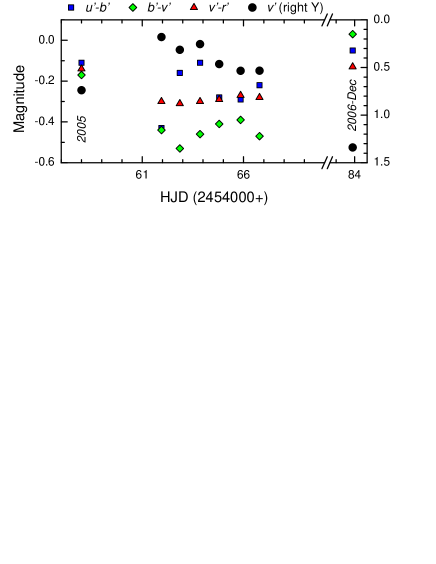
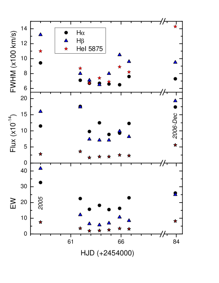
Figure 3: The $u^{\prime}-b^{\prime}$, $b^{\prime}-v^{\prime}$ and $v^{\prime}-r^{\prime}$ colour indices observed in BF Eri. Symbols represent data obtained from the night-averaged spectra. The $v^{\prime}$ light curve is also shown (dots, right Y).

Figure 4: Equivalent Width (EW), line fluxes and Full Widths at Half Maximum (FWHM) variations of the H$\alpha$, H$\beta$ and He i $\lambda 5875$ emission lines observed in BF Eri.

Figure 5: Lomb-Scargle power spectrum of the H$\alpha$ radial velocity variations from the 2006 dataset. The inset shown is blow-up of the most prominent peak of the CLEANed power spectrum of the combined data.

3.4 The radial velocity of the white dwarf

In CVs the most reliable parts of the emission line profile for deriving the radial velocity curve are the extreme wings. They are presumably formed in the inner parts of the accretion disc and therefore should represent the motion of the WD with the highest reliability. We measured the radial velocities using the double-Gaussian method described by Schneider & Young (1980) and later refined by Shafter (1983). This method consists of convolving each spectrum with a pair of Gaussians of width $\sigma$ whose centres have a separation of $\Delta$. The position at which the intensities through the two Gaussians become equal is a measure of the wavelength of the emission line. The measured velocities will depend on the choice of $\sigma$ and $\Delta$, and by varying $\Delta$ different parts of the lines can be sampled. The width of the Gaussians $\sigma$ is typically set by the resolution of the data. In order to test for consistency in the derived velocities and the zero phase, we separately used the emission lines H$\alpha$ and H$\beta$ in the 2006-Nov phase-averaged spectra, and the emission line H$\alpha$ in the phase-averaged spectra from the 2005-N3 set. All measurements were made using a Gaussian FWHM of 100 ${\rm km~{}s^{-1}}$ (and also of 50 ${\rm km~{}s^{-1}}$ for the 2006 dataset) and different values of the Gaussian separation $\Delta$ ranging from 300 km s^-1 to 2000 km s^-1 in steps of 50 km s^-1, following the technique of “diagnostic diagrams” (Shafter, Szkody, & Thorstensen, 1986).

For each value of $\Delta$ we made a non-linear least-squares fit of the derived velocities to sinusoids of the form

$$V(\phi,\Delta)=\gamma(\Delta)-K_{1}(\Delta)\sin\left[2\pi\left(\phi-\phi_{0}\left(\Delta\right)\right)\right]$$ (1)

where $\gamma$ is the systemic velocity, $K_{1}$ is the semi-amplitude, $\phi_{0}$ is the phase of inferior conjunction of the secondary star and $\phi$ is the phase calculated relative to epoch $T_{0}=2453675.2670$ for the 2005-N3 set and $T_{0}=2454061.8112$ for the 2006-Nov set.

The resulting “diagnostic diagram” for H$\alpha$ in the 2006 dataset, with $\sigma=100$ km s^-1, is shown in Fig. 6. The diagram shows the variations of $K_{1}$, $\sigma(K_{1})/K_{1}$ (the fractional error in $K_{1}$), $\gamma$ and $\phi_{0}$ with $\Delta$ (Shafter, Szkody, & Thorstensen, 1986). The diagrams for other lines and $\sigma$ look the same. To derive the orbital elements of the line wings we took the values that correspond to the largest separation just before $\sigma(K_{1})/K_{1}$ shows a sharp increase (Shafter & Szkody, 1984). We find the maximum useful separation to be $\Delta\simeq 1100{-}1250$ ${\rm km~{}s^{-1}}$. In Fig. 6 it appears that $\Delta$ can be increased to $\sim$1150–1250 km s^-1 before $\sigma(K)/K$ begins to increase. We also note that all the calculated orbital elements are very stable, even for the smaller separation $\Delta$, hence there are no difficulties in choosing their values. This statement is also true for other “diagnostic diagrams”. We have obtained very consistent results for both the radial velocity semi-amplitudes and the $\gamma$-velocities for all of them, and we adopt the mean values $K_{1}=74\pm 3$ km s^-1 and $\gamma=-91\pm 7$ km s^-1. The measured parameters of the best fitting radial velocity curves are summarized in Tables 3 and 5. In Fig. 7 we show the radial velocity curves for the H$\alpha$ emission line.

The derived value of the radial velocity semi-amplitude $K_{1}$ is highly inconsistent with the one found by Sheets et al. (2007). We are unable to explain why their result is so different, as they did not present their analysis in detail. On the other hand, we have no reason to doubt our values. A possible reason might be poor spectral resolution for their data and as a consequence the wider Gaussians used in the double-Gaussian method. According to the “diagnostic diagram” (Fig. 6) we presume that Sheets et al. (2007) examined the lower-velocity parts of the H$\alpha$ line and consequently obtained a higher value of $K_{1}$.

Figure 6: The diagnostic diagram for the H$\alpha$ 2006-Nov data, showing the response of the fitted orbital elements to the choice of the double-gaussian separation. The best fit is reached with the gaussian separation of 1150–1250 km s^-1.

Table 3: Elements of the radial velocity curves of BF Eri derived from emission lines

Emission line &	K1	$\gamma$-velocity a	$\phi_{0}$b
dataset	(km s-1)	(km s-1)
H$\alpha$ - 2005	74$\pm$4	-98$\pm$4	0.013$\pm$0.011
H$\alpha$ - 2006	74$\pm$4	-66$\pm$5	0.012$\pm$0.015
H$\beta$ - 2006	77$\pm$10	-73$\pm$12	0.013$\pm$0.016
Mean	74$\pm$3	-91$\pm$7	0.0127$\pm$0.0003

^a The measured $\gamma$-velocities are heliocentric. The mean value was obtained after correction for the solar motion.
^b Phases were calculated relative to epoch $T_{0}=2453675.2670$ for the 2005 set and $T_{0}=2454061.8112$ for the 2006 set.

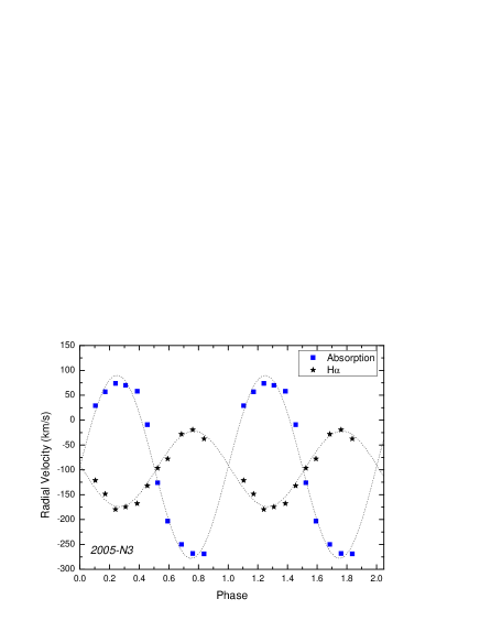
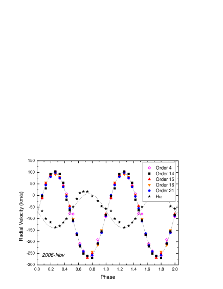
Figure 7: Radial velocities of the white dwarf and the secondary star in BF Eri folded on the ephemeris from Table 5. Observations were performed in 2005 November (left panel) and 2006 November (right panel). Two cycles are shown for clarity.

3.5 The radial velocity of the secondary star

The absorption lines from the secondary star in BF Eri are visible quite clearly, even in the individual spectra of the 2005-N3 set, and more easily in the phase-folded spectra of both the 2005-N3 and 2006-Nov sets. In order to obtain radial velocities, we used the following interactive method.

1. The first step was to measure the radial velocity variations of the absorption line Ca i $\lambda$6162 (and the Fe i/Ca i/Ba i $\lambda$6495 blend for comparison purpose) in the phase-folded spectra of the 2005-N3 set. The velocities were measured by convolving the observed line profiles with a single Gaussian. The resulting radial velocity curves were then fitted with a sinusoid of the form

   $$V(\phi)=\gamma-K_{2}\sin\left[2\pi\left(\phi-\phi_{0}\right)\right]$$ (2)

   and preliminary values of the radial velocity semi-amplitude $K_{2}$, the systemic velocity $\gamma$ and the phase zero-point $\phi_{0}$ were calculated. The obtained parameters are $K_{2}=183\pm 6$, $\gamma=-94\pm 5$ and $\phi_{0}=0.561\pm 0.007$.

2. Each spectrum in both the 2005-N3 and 2006-Nov sets was then shifted to correct for the orbital motion of the donor star, and the results averaged. These averaged spectra of BF Eri in the rest frame of the secondary star allowed us to estimate a preliminary spectral type of the donor star (see Section 3.6). The averaged spectra of BF Eri were then cross-correlated with the velocity standards of the obtained spectral type and the relative shifts computed and applied.

   Thus, we obtained the cross-correlation template spectra which were used for measuring the absorption-line velocities. This was preferable to cross-correlating with the standard stars for the obvious reason that it maximizes the similarity between the template and the individual spectra to be cross-correlated, and avoids introducing errors caused by spectral-type mismatch between the standard star and the secondary star in BF Eri, as well as by the incorrectly determined rotational broadening of the absorption lines.

3. Next, the phase-folded BF Eri spectra were cross-correlated with the templates. For the 2005-N3 set, the wavelength region 6150–6515 Å was used. To avoid the influence of the night-sky lines $\lambda$6300 Å and $\lambda$6363 Å, some portions of the spectral range around these lines were blanked. For the Echelle 2006-Nov set, the procedure was carried out using orders 4, 14, 15, 16 and 21 in the wavelength regions 4220–4235 Å, 5160–5235 Å, 5260–5400 Å, 5360–5500 Å and 6100–6270 Å respectively (Fig. 2). The solutions obtained by fitting the measured radial velocities with sinusoid (2) are very similar for both sets and all orders.

4. Steps 2 and 3 were then repeated and the final results (with almost no changes from the previous step) were obtained, so we adopt the averaged values of $K_{2}=182.5\pm 0.9$ km s^-1 and $\gamma=-93.6\pm 0.4$ km s^-1. These values are consistent with Sheets et al. (2007). We also note that the difference between the phase zero-points obtained from the emission and absorption lines is very close to 0.5, as it must be if the derived velocities from those lines trace the components’ motion. In Fig. 7 we show the measured radial velocities together with their sinusoidal fit. The measured parameters of the best fitting radial velocity curves are summarized in Tables 4 and 5.

5. Finally, the step 3 was repeated again, using the standard templates of the best-fitting spectral type K3V broadened to the predicted rotational velocity of the mass donor $V_{rot}\sin i$=78 km s^-1 (see Section 3.7 and footnote 2 for details). No significant difference in the measured parameters was found.

Table 4: Elements of the radial velocity curves of BF Eri derived from absorption lines by means of cross-correlation.

Dataset	Spectral	Wavelength	K2	$\gamma$-velocity a	$\phi_{0}$b
	Order	region (Å)	(km s-1)	(km s-1)
2005		6150–6515	185$\pm$5	-94$\pm$4	0.500$\pm$0.005
2006	Order 04	4220–4235	180$\pm$4	-80$\pm$3	0.502$\pm$0.003
2006	Order 14	5160–5235	187$\pm$3	-83$\pm$2	0.499$\pm$0.002
2006	Order 15	5260–5400	183$\pm$2	-81$\pm$1	0.499$\pm$0.001
2006	Order 16	5360–5500	182$\pm$2	-81$\pm$2	0.500$\pm$0.002
2006	Order 21	6100–6270	181$\pm$2	-82$\pm$1	0.499$\pm$0.001
Mean			182.5$\pm$0.9	-93.6$\pm$0.4	0.500$\pm$0.001

^a The measured $\gamma$-velocities are heliocentric. The mean value was obtained after correction for the solar motion.
^b Phases were calculated relative to epoch $T_{0}=2453675.2670$ for the 2005 set and $T_{0}=2454061.8112$ for the 2006 set.

3.6 Spectral type of the secondary star

The best absorption lines for spectral classification in normal stars, which are independent of chemical abundances are the line ratios of the Fe i lines $\lambda 4250$, $\lambda 4260$, $\lambda 4271$ to the Cr i lines $\lambda 4254$ and $\lambda 4274$, as well as the strength of the Ca i $\lambda$4226 line (Keenan & McNeil, 1976; Echevarría et al., 2007). The Cr i lines increase in strength with respect to the Fe i lines with spectral type. On the other hand the intensity of the Ca i line also increases steadily as the spectral type advances (in fact this line has a saturation effect for late K and M stars). Unfortunately, due to the poor sensitivity of the CCD at short wavelengths the data were too noisy in this wavelength region, so we were able to use only the width of the Ca i $\lambda$4226 line as a spectral indicator. In accordance with this a spectral type of the secondary star in BF Eri can be initially estimated as K3–K4.

To verify this result, we also analyzed the appearance of the absorption lines in those spectral orders where they are visible better. Purely by inspection, we have found several reliable indicators to be useful in constraining the spectral type. Among them are pairs of the lines/blends Fe i $\lambda$5227.2 and Cr i/Fe i $\lambda$$\lambda$5206+5208 (order 14), Fe i $\lambda$5434.5 and Fe i $\lambda$5424.1 (order 16), Ca i $\lambda$6122.2 and Fe i $\lambda$6137 (order 21), Ca i $\lambda$6439.1 and Fe i $\lambda$$\lambda$6400.0+6400.3 (order 22). The relative depths of all these couples change rapidly over the spectral type range we are interested in here. Analysis of these absorption features supports a K2–K3 spectral classification for the donor star in BF Eri.

Taking into account all the estimations we adopt the final value for the spectral type of the secondary to be K3$\pm$0.5, consistent with the determination of Sheets et al. (2007).

3.7 Rotational velocity of the secondary star

The absorption lines visible in the averaged and orbitally corrected spectra are obviously broadened due to orbital smearing during exposure and rotation of the secondary star. The observed rotational velocity of the secondary could provide an independent determination of the mass ratio of the binary. We have attempted to estimate this parameter by artificially broadening the template star spectra which are assumed to have low $V_{rot}\sin i$, and fitting them to the orbital velocity corrected BF Eri spectra until the lowest residual was obtained. We have restricted this analysis to the spectra acquired with the Echelle spectrograph because of their higher spectral resolution. We have selected from them those spectral orders which exhibit the greater set of the strong absorption-line features (orders 14, 15, 16 and 21). All details of the used $V_{rot}\sin i$ measuring technique can be found in Smith, Dhillon, & Marsh (1998) [see also Marsh, Robinson, & Wood (1994) and North et al. (2000)].

Unfortunately, despite the efforts expended we have failed to derive consistent value for the rotational velocity. Instead we obtain a quite broad range of $V_{rot}\sin i$ values of 70–100 km s^-1, that is unacceptable for the determination of the system parameters. We have additionally examined the spectra, varying the wavelength ranges and even cutting the separate absorption lines, but were unable to get a more certain value of $V_{rot}\sin i$. We explain our failure by the insufficient quality of the used spectra as even the averaged spectra are quite noisy. We still need more observations with high spectral resolution and better time resolution to fully solve this problem.

Although we could not determine the rotational velocity, we were able to estimate the fractional contribution of the secondary star to the total light. We have found that the secondary contributes about 11 per cent of the total light in order 14.

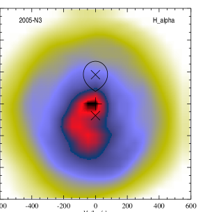
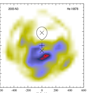
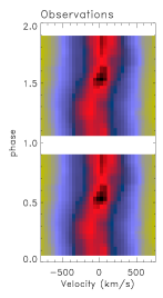
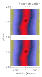
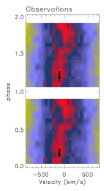
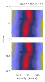
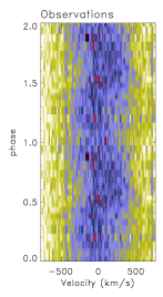
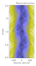
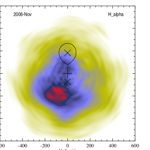
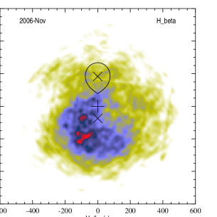
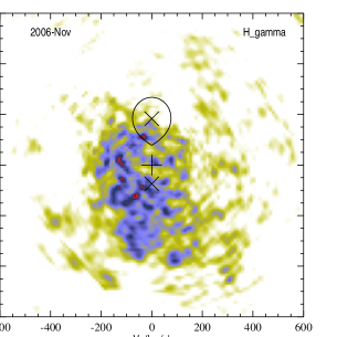
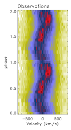
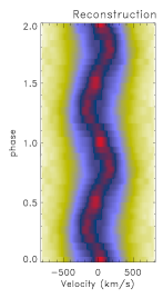
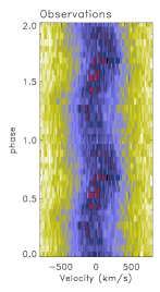
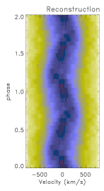
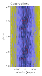
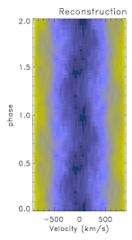
Figure 8: Doppler tomography for the H$\alpha$ and He i $\lambda$6678 emission lines from the 2005-N3 set and for the He i $\lambda$5876 line from the 2006-Nov set (in the upper half of Figure), and for H$\alpha$, H$\beta$ and H$\gamma$ from the 2006-Nov set of observations (in the bottom half of Figure). For each line the observed and reconstructed trailed spectra (bottom) and corresponding Doppler maps (top) are shown.

4 Doppler Tomography

The orbital variation of the emission line profiles indicates a non-uniform structure for the accretion disc. In order to study the emission structure of BF Eri we have used Doppler tomography. Full technical details of the method are given by Marsh & Horne (1988) and Marsh (2001). Examples of the application of Doppler tomography to real data are given by Marsh (2001).

Figure 8 shows the tomograms of the H$\alpha$ and He i $\lambda$6678 emissions from the 2005-N3 set and of the H$\alpha$, H$\beta$, H$\gamma$ and He i $\lambda$5876 emissions from the 2006-Nov set of observations, computed using the code developed by Spruit (1998). These figures also show trailed spectra in phase space and their corresponding reconstructed counterparts. A help in interpreting Doppler maps are additional inserted plots which mark the positions of the WD (lower cross), the center of mass of the binary (middle cross) and the Roche lobe of the secondary star (upper bubble with the cross). The Roche lobe of the secondary has been plotted using the system parameters, derived in Section 5.

Due to the non-double-peaked emission line profiles of BF Eri, we did not expect a Doppler map to have an annulus of emission centered on the velocity of the WD, and the observed tomograms do not show it. Instead of this all the maps display a similar, very nonuniform distribution of the emission, the bulk of which is located in the lower-left quadrant of the tomograms, at lower velocities than the predicted outer disc velocities for an accretion disc with a radius $R_{L_{1}}$. The appearance of the 2005-N3 H$\alpha$ map is similar to the hydrogen line maps from the 2006-Nov set but a most prominent contribution of the emission here is from the area around the center of mass of the binary system. Note also that BF Eri does not show any emission on the hemisphere of the donor star facing the WD and boundary layer.

The interpretation of the emission structure in BF Eri is ambiguous. All the detected emission sources are located far from the region of interaction between the stream and the disc particles. This ’reversed bright spot’ phenomenon can perhaps be explained by a gas stream which passes above the disc and hits its back (Hellier & Robinson, 1994), or alternatively, by the disc thickening in resonating locations.

5 The binary system parameters

It is impossible to determine accurate system parameters for a non-eclipsing binary system like BF Eri. However, we can constrain them, using the measurements of the radial velocities of the primary and secondary stars $K_{1}$ and $K_{2}$ in conjunction with the derived orbital period $P_{orb}$ and the spectral class of the secondary.

Combining the values of $K_{1}$, $K_{2}$ and $P$ we find the masses of each component of the system

$$M_{1}\sin^{3}i={PK_{2}(K_{1}+K_{2})^{2}\over 2\pi G}=0.34\pm 0.01M_{\odot}\,,$$ (3)

$$M_{2}\sin^{3}i={PK_{1}(K_{1}+K_{2})^{2}\over 2\pi G}=0.14\pm 0.01M_{\odot}\,,$$ (4)

and the projected binary separation

$$a\sin i={P(K_{1}+K_{2})\over 2\pi}=1.37\pm 0.02R_{\odot}\,.$$ (5)

The inclination angle $i$ of the system is an unknown parameter but for a CV it can be restricted by using some reasonable assumptions. The published photometry of BF Eri is extensive enough to rule out any significant eclipse, which constrains the inclination $i$ to be less than about 70^∘ to avoid an obvious partial eclipse of the disc. At $i$ = 70^∘ the minimum WD mass is around 0.41 $M_{\odot}$. The Chandrasekhar mass limit determines the lowest limit for the inclination angle to be about 38^∘. Thus, we have now the pure dynamic solution for the parameters of BF Eri: $q\equiv M_{2}/M_{1}=K_{1}/K_{2}=0.41\pm 0.02$, $M_{1}$=0.41–1.44 $M_{\odot}$, $M_{2}$=0.17–0.59 $M_{\odot}$, $i$=38^∘–70^∘, $a$=1.46–2.23 $R_{\odot}$.

At this point we would like to take note that from general theoretical considerations the donor star in a long-period CV should be more massive than in a short-period one. In practice, using any of the recently obtained empirical mass-period relations (see, for example, Warner 1995; Smith & Dhillon 1998; Patterson et al. 2005) we obtain the mass for the secondary 0.67–0.72 $M_{\odot}$ (Fig. 9, bottom panel). This is even more than our upper bound for the donor mass, leading us to the conclusion that the WD in BF Eri is very close to the Chandrasekhar limit.

Also we can estimate the secondary’s mass, reasonably assuming that the secondary star fills its Roche lobe. The relative size of the donor star is constrained by Roche geometry and can be estimated using Eggleton’s formula (Eggleton, 1983)

$$\frac{R_{2}}{a}=\frac{0.49q^{2/3}}{0.6q^{2/3}+\ln(1+q^{1/3})},$$ (6)

which gives the volume-equivalent radius of the Roche lobe to better than 1 per cent.

In Fig. 9 (upper panel) we show the Roche lobe size of the secondary as a function of the binary separation, and also different theoretical and empirical Mass-Radius relations. One can see that in order to fill its Roche lobe, the secondary must be relatively massive (0.7–0.8 $M_{\odot}$) if it is on the main sequence. But the mass of the primary in this case must exceed the Chandrasekhar limit, contradicting observations. A very massive white dwarf might just be accommodated again. However the secondary of the corresponding mass of 0.59 $M_{\odot}$ must be significantly larger than a main-sequence star of the same mass. It is now well known that all CVs have secondaries slightly larger ($\sim 15$ per cent) than the zero-age main-sequence (ZAMS) single-star (Patterson et al., 2005; Knigge, 2006) but the secondary in BF Eri is even greater by another 15 per cent.

Additional constrains on the mass of the secondary can be obtained using another independently obtained parameter – its spectral type. Actually, this method should be used with great caution as it is understood that there is a big range in mass for a given spectral type (Smith & Dhillon, 1998). However, using the latest generation of low-mass star models, Kolb, King, & Baraffe (2001) explored theoretically to what extent the spectral type provides a reasonable estimate of the donor mass. They concluded that the spectral type should be a good indicator of the donor mass, and gave lower and upper limits to $M_{2}$ for a given spectral type (see Table 1 in their paper). For the secondary star in BF Eri we have the range of masses of $\sim 0.5-0.8M_{\odot}$. The upper limit here is for the mass of a ZAMS star with the same spectral type as the donor while the lower limit is for evolved main sequence stars under some extreme assumptions as discussed by Kolb, King, & Baraffe (2001). Thus, this leads us to conclude that the secondary in BF Eri is an evolved star of the mass of $\sim 0.50-0.59M_{\odot}$. This in turn explains why the size of the secondary is so big for its mass. As Baraffe & Kolb (2000) showed, the size of the donor star of any given mass is larger for more evolved sequences.

Thus, from the above analysis based on strong assumptions, we can restrict the system parameters of BF Eri in the following ranges: $q$=0.41, $M_{1}$=1.23–1.44 $M_{\odot}$, $M_{2}$=0.50–0.59 $M_{\odot}$, $i$=38^∘–40.5^∘, $a$=2.11–2.23 $R_{\odot}$. Finally, in order to esimate the “best-fitting” values of the component masses and their errors, we used a Monte Carlo approach similar to Horne, Welsh, & Wade (1993). The Monte Carlo simulation takes $10^{6}$ sample values of $K_{1}$ and $K_{2}$, treating each as being normally distributed about their measured values with standard deviations equal to the errors on the measurements. The values of the inclination $i$ are sampled at random from an uniform distribution over the interval [0, $i_{max}$], where $i_{max}=70^{\circ}$. Using the relations (3) and (4), we then calculate the masses of the components. If $M_{1}$ exceeds 1.44 $M_{\odot}$, or $M_{2}$ is less than 0.50 $M_{\odot}$, the outcome is rejected. The ensuing distribution for accepted outcomes is used to calculate the component masses. The values of all the system parameters deduced from the Monte Carlo simulation are listed in Table 5. Each value corresponds to the peak and standard deviation of the relevant distribution.

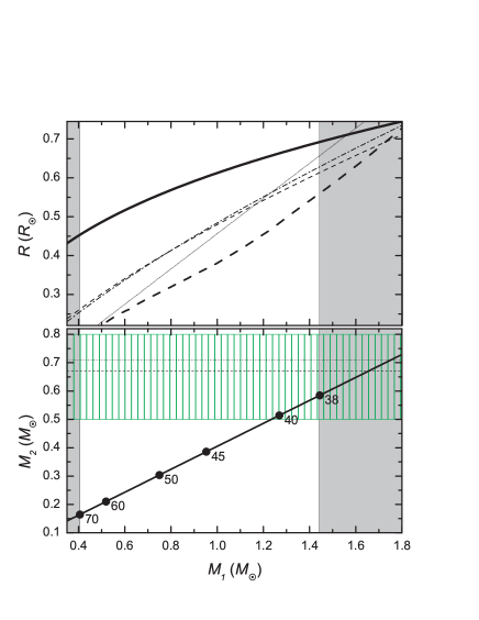
Figure 9: Constraints on the system parameters of BF Eri. In the bottom panel, we show the $M_{1}$ – $M_{2}$ diagram. The diagonal solid line correspond to the derived mass ratio $q$=0.41. The dots along this line correspond to different mass solutions for specific values of the inclination angle, labelled nearby to those dots. The two vertical areas (shown in grey) mark the regions of impossible values, due to lack of eclipses (on the left) and the Chandrasekhar mass limit (on the right). The two horizontal lines show the predicted mass of the secondary from the $M_{2}$–$P_{orb}$ relations by Warner (1995) and Patterson et al. (2005) (the dashed and dotted lines, respectively). The green vertical line pattern circumscribes the range of masses of the evolved main sequence star of the spectral type K3 under some extreme assumptions as discussed by Kolb, King, & Baraffe (2001). In the upper panel we show, by the thick solid line, the Roche lobe size of the secondary $R$ as a function of the mass of the WD $M_{1}$, for the mass ratio $q$=0.41 and $P_{orb}$=0.270881 days. The lower lines correspond to different theoretical and empirical Mass-Radius relations. The thick dashed line is the theoretical $M$-$R$ relation of Baraffe et al. (1998). The thin dashed and dash-dotted lines are the empirical relations of Knigge (2006) and Patterson et al. (2005) respectively. The short-dotted line is the $M$-$R$ relation based on photometric, geometrical, and absolute elements for 112 eclipsing detached binary systems with both components on the main sequence and with known photometric and spectroscopic orbital elements (Gorda & Svechnikov, 1998).

Table 5: Orbital and system parameters for BF Eridani.

Parameter	Measured	Monte Carlo
	Value	Value
$P_{orb}$ (d)	0.270881$\pm 3\times 10^{-6}$
$T_{0}$ (+2450000)	4061.8112$\pm$0.0003
$K_{1}$ (km s-1)	74$\pm$3
$K_{2}$ (km s-1)	182.5$\pm$0.9
$\gamma$ (km s-1)	-93.6$\pm$0.4
Spectral Type
of secondary	K3$\pm$0.5
$d$ (pc)	700$\pm$200
$M_{1}/M_{\sun}$	1.23–1.44	1.28$\pm$0.05
$M_{2}/M_{\sun}$	0.50–0.59	0.52$\pm$0.01
$q=M_{2}/M_{1}$	0.41$\pm$0.02	0.41$\pm$0.01
$i$	38∘–40.5∘	40${}^{\circ}\pm$1
$a/R_{\sun}$	2.11–2.23	2.14$\pm$0.02

6 Discussion

6.1 System parameters

We would like to make some final remarks on the system parameters of BF Eri, derived in Section 5. These parameters were determined using a traditional spectroscopic solution based on the derived radial velocity semi-amplitudes. In order to calculate the masses of the binary we have assumed that the semi-amplitudes of the measured radial velocities represent the true orbital motion of the stars. In CVs, however, this may not be an accurate assumption, as the emission lines arising from the disc may suffer several asymmetric distortions. Likewise, absorption line profiles may be subjected to irradiation or hot-spot contaminations in the surface of the secondary, distorting therefore the true value of $K_{2}$.

Taking these potential sources of errors into consideration we, however, believe we could avoid them. Indeed, though those problems were severe in the early determinations of the radial velocities, nevertheless modern high resolution spectroscopy has greatly improved the methods in detecting asymmetric distortions to provide more reliable radial velocity values (Warner, 1995). In our study of BF Eri, the value of $K_{2}$ is beyond question. Scattering of its values derived with the use of the different data, is very small. Doppler tomography does not show any emission from the secondary star that can distort the absorption line profiles from the latter, neither in quiescence nor in the outburst. Furthermore, a non-uniform absorption distribution across the surface of the secondary would result in a non-sinusoidal radial velocity curve that is not observed in BF Eri (Fig. 7). All the obtained values of $K_{1}$ are also consistent with each other. Though the detected asymmetric emission structure of BF Eri (particularly, the spot in the lower-left of the Doppler maps) may potentially influence the velocity determination, we believe we could avoid this as that strong emission spot is situated well inside of the chosen Gaussian separation. The correct phasing of the radial velocity curve also strengthens our confidence.

Alternatively, one may also calculate the mass ratio of BF Eri using the observed rotational velocity of the secondary star, independently of $K_{1}$. Unfortunately, we were unable to derive a consistent value of the rotational velocity, getting instead a broad range of $V_{rot}\sin i$ values. This gives us the $q$ values in the range of 0.33–0.62 that is consistent with the former solution, but also very uncertain, so we decided to reject it.

Thus, we have shown that BF Eri contains a massive WD and an evolved secondary. This places this system among a small group of CVs with a high-mass WD (such as RU Peg and U Sco). Such systems are specially interesting since they are considered as possible Type Ia supernova progenitors (Parthasarathy et al. 2007, and references therein). The identity of the progenitor has become important for cosmology, since Type Ia supernovae are used as standard candles and their peak luminosity depends on the nature of the progenitor. The exploding star is now thought to be a carbon–oxygen WD that accretes mass from a binary companion until it approaches the Chandrasekhar limit, ignites carbon under electron-degenerate conditions, undergoes a thermonuclear instability, and disrupts completely. Further studies of the systems with massive WDs similar to BF Eri are needed to understand if they evolve to SNe Ia.

6.2 $\gamma$-velocity, proper motion and distance

A decade ago van Paradijs, Augusteijn, & Stehle (1996) drew attention to the distribution of space velocities, as a means of probing the age profile of the CV population. Kolb & Stehle (1996) derived the theoretically expected distribution of $\gamma$-velocities and the dispersion of $\gamma$ as a function of orbital period. In particular, they showed that the CVs having periods longer than the upper limit of the period gap ($P_{orb}\geq$3 h) should be younger ($\leq$1.5 Gyr), and therefore have a smaller line-of-sight velocity dispersion according to the empirical age-velocity dispersion relation (predicted value $\sim$15 km s^-1). Conversely, those CVs with orbital periods shorter than the lower limit of the period gap, should be older ($\geq$ 3–4 Gyr) and show a larger velocity dispersion (predicted as $\sim$30 km s^-1). Paying a special attention to determine accurate absolute systemic velocities, North et al. (2002) found its values for four long-period DNs. They obtained an average $\gamma$-velocity of $\sim$5 km s^-1 with a dispersion of $\sim$8 km s^-1  indicating that the above postulate is indeed true.

In our study of BF Eri, we have mostly followed the method of North et al. (2002) and found the absolute $\gamma$-velocity, after correction for the solar motion, to be $-94$ km s^-1, referred to the dynamical local standard of rest (LSR). This value is very far away from any expectations of the theory (as set out by Kolb & Stehle 1996). In principle, such a kick velocity could be caused by an event in which a significant fraction of the total mass of the system is violently, asymmetrically ejected. In the case of CVs, the progenitors indeed eject most of their mass during the common-envelope period, but it is supposed that this process does not alter the space velocity of the system. Kolb & Stehle (1996) note, however, that this velocity may be affected by the cumulative effect of repeated nova eruptions with asymmetric envelope ejection.

It is worthy to mention that BF Eri shows not only the high $\gamma$-velocity but also has a substantial proper motion: $(\mu_{x},\mu_{y})=(+34,-97)$ mas yr^-1(Klemola, Hanson, & Jones, 2000; Hanson et al., 2004). In order to convert this value to the space velocity we need to know the distance to the system, which we can evaluate here by oblique methods only.

One of these estimations is based on the statistical period-luminosity-colours relation of Ak et al. (2007). We have taken the $JHK$ magnitudes of BF Eri from the 2MASS (Two Micron All Sky Survey) observations (Hoard et al., 2002; Skrutskie et al., 2006) and found the distance to the system, from the dependence of the absolute magnitude $M_{J}$ on the orbital period $P_{orb}$ and colours $(J-H)$ and $(H-K_{s})$, to be $700\pm 200$ pc.

Alternatively, the distances can be estimated based on a semi-empirical donor sequence for CVs of Knigge (2006). Unfortunately, Knigge’s donor sequence is intended to describe the unique evolution track followed by unevolved secondaries, and he limited it to $P_{orb}\la 6.2$ h. BF Eri is a system with a longer period and likely an evolved secondary. However, we have slightly extrapolated Knigge’s sequence and found from it and the $JHK$ magnitudes the lower limit of the distance $d$ to be $\sim 500$ pc. Applying the empirical offsets to the donor absolute magnitudes (see, however, comments by Knigge on this) we have obtained $d$ to be $\sim 900$ pc.

Finaly, the distances can also be derived from the absolute magnitude at outburst $M_{V}$(max) versus the orbital period relation of Harrison et al. (2004), if one intends to consider the flares of BF Eri as DN outbursts (see corresponding discussion in Section 6.3). Analysis of the AAVSO database of BF Eri’s observations reveals 8 events brighter than 13 mag with an averaged value of $12.5\pm 0.2$ mag. This yields the distance to be $650\pm 60$ pc.

Fortunately, all these independent estimations of the distance are consistent with each other, leading us to a final value of $700\pm 200$ pc. This corresponds to a transverse velocity $v_{T}=340\pm 100$ km s^-1 or a space velocity of $\sim$350 km s^-1 with respect to the LSR, that is again unusually high. Based on kinematics, Sheets et al. (2007) surmised that BF Eri may belong to the halo population. Our Galactic components of the space velocity of the system $(U,V,W)=(-220,-280,4)$ km s^-1are slightly different from those obtained by Sheets et al. but also support a system motion being essentially in the Galactic plane and lagging far behind the rotation of the Galactic disc. In this connection the referee has pointed out that the high space velocity may be simply a sign of great age and not a result of any asymmetric mass ejections, that would be consistent with the secondary star having started to evolve prior to the time the system came into contact. Indeed, though Kolb & Stehle (1996) do mention asymmetric nova explosions as a possible mechanism for increasing the dispersion in the $\gamma$-velocity distribution, but they give no numbers, and it is not yet clear whether it is really plausible that the effect could produce a $\gamma$-velocity as large as the one we found.

However, if such a high space velocity of BF Eri was indeed caused by repeated nova eruptions then it might be worth searching for its past (recurrent) nova outbursts in the astronomical archive. Although the system is known only since 1940 and during the following 50 years there were no observations, some collections of photographic plates cover over a century of data. It is straightforward to look at plates taken over the years to see if past eruptions have been recorded.

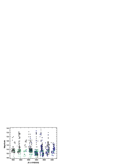
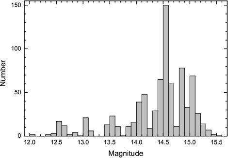
Figure 10: Left: The AAVSO light curve of BF Eri. Blue stars represent the data labelled in the AAVSO database as V-magnitude, black filled dots - as Visual-magnitude, open dots - as inaccurate Visual-magnitude, green triangles - as the “Fainter Than” Visual-data. Right: Histogram of the reliable AAVSO data for BF Eri.

6.3 The outburst behaviour and the nature of BF Eri

The current classification of BF Eri as a DN is based on observations by Watanabe and Kato (Watanabe, 1999; Kato, 1999; Kato & Uemura, 2000) who detected “outbursts” in the light curve of the system. We note that all those outbursts were of low amplitude (1–1.5 mag) forcing Kato to classify BF Eri as “a low-amplitude dwarf nova”. However from the formal side, DNs are an subset of CVs, which undergo recurrent outbursts of 2–8 mag. The observed “outbursts”, including the one observed during the 2006-Nov set, are of much lower amplitude, which leads us to the question: are those events the real DN outbursts rather than some kind of flares?

It is now widely accepted that the reason for a DN outburst is a thermal instability in the accretion disc, which switches the disc from a low-viscosity to a high-viscosity regime (Smak, 1984; Osaki, 1996; Lasota, 2001). From the observational side this is (usually) accompanied by substantial spectral changes occurring continuously during all stages of the outburst. More than half of DNs exhibit the transition from emission-line spectrum at quiescence to absorption-line spectrum at maximum. For the rest if any emission can be seen it is often in the form of emission lines buried in absorption troughs (Warner, 1995; Morales-Rueda & Marsh, 2002). Quite often the spectral line profiles undergo dramatic changes as new emission sources arise in the system such as the inner hemisphere of the secondary star. This emission is caused by increased irradiation from the accretion regions during the outburst and can be seen in hydrogen and neutral helium lines through Doppler tomography (Neustroev, Zharikov, & Michel, 2006). Many systems show also strengthening of the He ii and C iii/N iii line emissions during an outburst.

None of these outburst signs was observed in BF Eri. Thus the observed flares can hardly be associated with a DN outburst. This in turn raises a question on the classification of the system. Actually, BF Eri does not also show many other usual observational signs of DNs. For example, in spite of the high spectral resolution used, all the emission lines show not the double-peaked profiles but single-peaked ones. From the above-estimated system parameters we can expect the double peak separation to be more than 500 km s^-1, that is more than enough to be resolved. However, though the profiles are highly variable, they do not show any signs of the double-peaked accretion disc structure. In consequence, a ring-like emission distribution, characteristic of a Keplerian accretion disc about the WD, is also absent from the Doppler maps. On the other hand, the bulk of the Balmer emission is located to the lower left quadrant of the tomograms. Both the emission line profiles and the appearance of the Doppler maps resemble those in nova-like CVs which in turn resemble those typical for old novae at minimum light.

By definition, NLs should not display any DN outbursts. Their almost steady brightness is thought to be due to their mass transfer rate $\dot{M}$ exceeding the upper stability limit $\dot{M}_{crit}$. These stars are thus thermally and tidally stable. However, Honeycutt, Robertson, & Turner (1998) reported that a significant fraction of NLs displays so-called “stunted” outbursts. Honeycutt (2001) found many similarities between them and outbursts in ordinary DNs but the former are of much smaller amplitude (0.4–1 mag). We suppose thus that BF Eri might be a NL system exhibiting “stunted” outbursts.

The AAVSO database has almost fourteen hundred BF Eri observations obtained largely after 1999 (Henden, 2007). We have analyzed the light curve compiled from the ‘Visual magnitude’ and ‘V magnitude’ data and found that the outburst activity of BF Eri is quite complex (Fig. 10, left). Histogram of the AAVSO data reveals at least three types of flashes (Fig. 10, right). Besides the above-mentioned low-amplitude flashes with the peak magnitude $\sim$13.0 mag and $\sim$13.5 mag, there were also 8 events with the amplitude more than 1.6 mag but always less than 2.3 mag, with $V_{max}\approx 12$. Formally, the brightest flashes lie on the bottom edge of the accepted range of the outburst amplitudes in ordinary DNs and might be such outbursts. The nature of the low-amplitude flashes is still unclear; further investigation is needed.

Finally, we have obtained the periodogram, using the AAVSO data (Fig. 11). It shows significant excess power in the interval 60–90 d, reflecting a reliable stability of the flashes.

Figure 11: The Lomb-Scargle power spectrum of BF Eri, derived from the AAVSO data.

7 Summary

We have presented spectroscopic observations of the cataclysmic variable BF Eri during its low and bright states. The most important results of this study can be summarized as follows:

1. The orbital period of BF Eri is $P_{orb}=0.270881(3)$ days.

2. We have shown that BF Eri contains a massive WD ($M_{1}\geq 1.23M_{\odot}$). This allows us to consider the system as a SN Ia progenitor.

3. The spectral type of the secondary star is K3$\pm$0.5.

4. We have shown that the secondary in BF Eri is an evolved star of the mass of 0.50–0.59 $M_{\odot}$, whose size is about 30 per cent larger than a ZAMS star of the same mass.

5. BF Eri shows the high $\gamma$-velocity ($\gamma=-94$ km s^-1) and substantial proper motion. With our estimation of the distance to the system ($d\approx 700\pm 200$ pc), this corresponds to a space velocity of $\sim$350 km s^-1 with respect to the LSR. The cumulative effect of repeated nova eruptions with asymmetric envelope ejection might explain the high space velocity of the system.

6. We have analyzed the outburst behaviour of BF Eri and question the current classification of the system as a dwarf nova. We propose that BF Eri might be an old nova exhibiting “stunted” outbursts.

References

- Ak et al. (2007) Ak T., Bilir S., Ak S., Retter A., 2007, NewA, 12, 446
- Baraffe et al. (1998) Baraffe I., Chabrier G., Allard F., Hauschildt P. H., 1998, A&A, 337, 403
- Baraffe & Kolb (2000) Baraffe I., Kolb U., 2000, MNRAS, 318, 354
- Chisholm et al. (1999) Chisholm J. R., Harnden F. R., Jr., Schachter J. F., Micela G., Sciortino S., Favata F., 1999, AJ, 117, 1845
- Echevarría et al. (2007) Echevarría J., Michel R., Costero R., Zharikov S., 2007, A&A, 462, 1069
- Eggleton (1983) Eggleton P. P., 1983, ApJ, 268, 368
- Elvis et al. (1992) Elvis M., Plummer D., Schachter J., Fabbiano G., 1992, ApJS, 80, 257
- Gorda & Svechnikov (1998) Gorda S. Y., Svechnikov M. A., 1998, ARep, 42, 793
- Hanley & Shapley (1940) Hanley C. M., Shapley H., 1940, BHarO, 913, 9
- Hanson et al. (2004) Hanson R. B., Klemola A. R., Jones B. F., Monet D. G., 2004, AJ, 128, 1430
- Harrison et al. (2004) Harrison T. E., Johnson J. J., McArthur B. E., Benedict G. F., Szkody P., Howell S. B., Gelino D. M., 2004, AJ, 127, 460
- Hellier & Robinson (1994) Hellier C., Robinson E. L., 1994, ApJ, 431, L107
- Henden (2007) Henden, A.A., 2007, Observations from the AAVSO International Database, private communication.
- Hoard et al. (2002) Hoard D. W., Wachter S., Clark L. L., Bowers T. P., 2002, ApJ, 565, 511
- Honeycutt (2001) Honeycutt R. K., 2001, PASP, 113, 473
- Honeycutt, Robertson, & Turner (1998) Honeycutt R. K., Robertson J. W., Turner G. W., 1998, AJ, 115, 2527
- Horne, Welsh, & Wade (1993) Horne K., Welsh W. F., Wade R. A., 1993, ApJ, 410, 357
- Kato (1999) Kato T., 1999, IBVS, 4745, 1
- Kato & Uemura (2000) Kato T., Uemura M., 2000, IBVS, 4882, 1
- Keenan & McNeil (1976) Keenan P. C., McNeil R. C., 1976, An atlas of spectra of the cooler stars: Types G,K,M,S, and C. Part 1: Introduction and tables (Columbus: Ohio State University Press)
- Klemola, Hanson, & Jones (2000) Klemola A. R., Hanson R. B., Jones B. F., 2000, Lick Northern Proper Motion Program: NPM1 Catalog (J2000 Version) (CDS Strasbourg Data Center Catalog No. I/199A), http://www.ucolick.org/ npm/NPM1
- Knigge (2006) Knigge C., 2006, MNRAS, 373, 484
- Kolb, King, & Baraffe (2001) Kolb U., King A. R., Baraffe I., 2001, MNRAS, 321, 544
- Kolb & Stehle (1996) Kolb U., Stehle R., 1996, MNRAS, 282, 1454
- Lasota (2001) Lasota J.-P., 2001, NewAR, 45, 449
- Levine & Chakrabarty (1995) Levine S., Chakrabarty D., 1995, IA-UNAM Technical Report #MU-94-04
- Lomb (1976) Lomb N. R., 1976, Ap&SS, 39, 447
- Marsh (2001) Marsh T. R., 2001, in Astrotomography, Indirect Imaging Methods in Observational Astronomy, ed. H. M. J. Boffin, D. Steeghs, and J. Cuypers, Lect. Notes Phys., 573, 1
- Marsh & Horne (1988) Marsh T. R., Horne K., 1988, MNRAS, 235, 269
- Marsh, Robinson, & Wood (1994) Marsh T. R., Robinson E. L., Wood J. H., 1994, MNRAS, 266, 137
- Morales-Rueda & Marsh (2002) Morales-Rueda L., Marsh T. R., 2002, MNRAS, 332, 814
- Neustroev, Zharikov, & Michel (2006) Neustroev V. V., Zharikov S., Michel R., 2006, MNRAS, 369, 369
- North et al. (2000) North R. C., Marsh T. R., Moran C. K. J., Kolb U., Smith R. C., Stehle R., 2000, MNRAS, 313, 383
- North et al. (2002) North R. C., Marsh T. R., Kolb U., Dhillon V. S., Moran C. K. J., 2002, MNRAS, 337, 1215
- Oke (1990) Oke J. B. 1990, AJ, 99, 1621
- Osaki (1996) Osaki Y., 1996, PASP, 108, 39
- Parthasarathy et al. (2007) Parthasarathy M., Branch D., Jeffery D. J., Baron E., 2007, NewAR, 51, 524
- Patterson et al. (2005) Patterson J., et al., 2005, PASP, 117, 1204
- Roberts, Lehar, & Dreher (1987) Roberts D. H., Lehar J., Dreher J. W., 1987, AJ, 93, 968
- Scargle (1982) Scargle J. D., 1982, ApJ, 263, 835
- Schachter et al. (1996) Schachter J. F., Remillard R., Saar S. H., Favata F., Sciortino S., Barbera M., 1996, ApJ, 463, 747
- Schneider & Young (1980) Schneider D. P., Young P., 1980, ApJ, 238, 946
- Shafter (1983) Shafter A. W., 1983, ApJ, 267, 222
- Shafter & Szkody (1984) Shafter A. W., Szkody P., 1984, ApJ 276, 305
- Shafter, Szkody, & Thorstensen (1986) Shafter A. W., Szkody P., Thorstensen J. R., 1986, ApJ, 308, 765
- Sheets et al. (2007) Sheets H. A., Thorstensen J. R., Peters C. J., Kapusta A. B., Taylor C. J., 2007, PASP, 119, 494
- Skrutskie et al. (2006) Skrutskie M. F., et al., 2006, AJ, 131, 1163
- Smak (1984) Smak J., 1984, PASP, 96, 5
- Smith & Dhillon (1998) Smith D. A., Dhillon V. S., 1998, MNRAS, 301, 767
- Smith, Dhillon, & Marsh (1998) Smith D. A., Dhillon V. S., Marsh T. R., 1998, MNRAS, 296, 465
- Spruit (1998) Spruit H. C., 1998, preprint (astro-ph/9806141)
- van Paradijs, Augusteijn, & Stehle (1996) van Paradijs J., Augusteijn T., Stehle R., 1996, A&A, 312, 93
- Warner (1995) Warner, B., 1995, Cataclysmic Variable Stars (Cambridge Astrophysics Ser. 28; Cambridge: Cambridge Univ. Press)
- Watanabe (1999) Watanabe, T., 1999, VSOLJ Variable Star Bulletin, 34