A robust statistical estimation of the basic parameters of single stellar populations. I. Method

Abstract

The colour-magnitude diagrams of resolved single stellar populations, such as open and globular clusters, have provided the best natural laboratories to test stellar evolution theory. Whilst a variety of techniques have been used to infer the basic properties of these simple populations, systematic uncertainties arise from the purely geometrical degeneracy produced by the similar shape of isochrones of different ages and metallicities. Here we present an objective and robust statistical technique which lifts this degeneracy to a great extent through the use of a key observable: the number of stars along the isochrone. Through extensive Monte Carlo simulations we show that, for instance, we can infer the four main parameters (age, metallicity, distance and reddening) in an objective way, along with robust confidence intervals and their full covariance matrix. We show that systematic uncertainties due to field contamination, unresolved binaries, initial or present-day stellar mass function are either negligible or well under control. This technique provides, for the first time, a proper way to infer with unprecedented accuracy the fundamental properties of simple stellar populations, in an easy-to-implement algorithm.

1 Introduction

The theory of stellar evolution has been tested extensively mainly through well-studied binary stars (e.g., Popper 1980, Lastennet & Valls-Gabaud 2002, Ribas 2006) or simple, coeval stellar populations such as open and globular clusters (e.g. Vandenberg et al. 1996, Renzini & Fusi Pecci 1988). It has been extraordinarily successful at explaining most stellar properties across the different evolutionary stages, by incorporating increasingly complex physics in both stellar interiors and atmospheres (see Salaris & Cassisi 2006 for an updated and extensive review). In contrast, and perhaps somewhat paradoxically, the determination of the fundamental parameters of single stellar populations, such as distance, age, metallicity, reddening, convective parameters, etc, has seldom been the subject of a rigorous mathematical determination. More often than not, isochrones are “fitted” by eye, and very rough estimates of errors are given, if given at all. The reason for this state of affairs is perhaps the many degeneracies between these parameters, which makes it seemingly impossible to find a unique solution to the set of fundamental parameters. Alternative, semi-empirical methods have been developed instead to infer relative quantities, rather than absolute ones. For instance, the so-called horizontal method relies on the difference in colour between the turn-off (TO) point and the base of the red giant branch (RGB), and is independent of the assumptions made on the convective theory. The vertical method, on the other hand, relies on the difference in apparent magnitude between horizontal branch (HB) stars and turn-off stars. Both methods rely heavily on “semi-empirical calibrations” provided by stellar models, and are subject to many uncertainties (e.g., How to define properly the TO point when photometric errors blur this region of the colour-magnitude diagram ? What is the vertical offset HB–TO when the HB is not horizontal ?) which nevertheless have been tackled with some success (e.g. Rosenberg et al. 1999, Salaris & Weiss 2002).

Here we want to point out that many of the degeneracies are actually mere artifacts, and that a proper and rigorous mathematical technique can be formulated to measure these parameters in a robust and objective way. For example, the well-known age-metallicity degeneracy, which states that a given isochrone can be fitted with a different age provided the metallicity is changed appropriately, is a purely geometrical degeneracy : the shape of the isochrones is the same, yet stellar evolution predicts that stars with a different metal content will evolve at a different speed. Hence, the age-metallicity degeneracy is not a physical one, but simply a result of using the geometrical shape of isochrones as the only discriminant factor. Clearly, a simple statistical estimator that would count the number of stars along the isochrones would give very different results for any pair of age/metallicity values that would give the same geometrical shape to the isochrones. In a more formal way, let us consider a curvilinear coordinate $s$ along an isochrone of given parameters (say, distance, reddening, metallicity, age, alpha elements enhancement, etc). This position depends only on the age $t$ of that isochrone and on the mass $m$ of the star at that precise locus, so that $s=s(m,t)$ only. An offset in age $dt$ is reflected only through changes in mass $m$ and position $s$ along the isochrone of age $t$ since

$$dt(m,s)\;=\;\left.\frac{\partial t}{\partial m}\right|_{s}\,dm\;+\;\left.\frac{\partial t}{\partial s}\right|_{m}\,ds\qquad.$$ (1)

For a star in this isochrone the offset is, by definition, zero, hence

$$\left.\frac{\partial m}{\partial s}\right|_{t}\;=\;-\;\left.\frac{\partial m}{\partial t}\right|_{s}\;\times\;\left(\left.\frac{\partial s}{\partial t}\right|_{m}\right)^{-1}\quad.$$ (2)

The first term is always finite. The second term is the evolutionary speed, the rate of change for a given mass $m$ of its coordinate along the isochrone when the age changes by some small amount. One can think of $s$ as representing some evolutionary phase, and so this term will be large when the phase is short-lived : a small variation in age yields a very large change in position along the isochrone. Alternatively, for a given age, and since the first term is always finite, a wide variation in position implies a narrow range in mass. This is the case of the red giant branch or the white dwarf cooling sequence, for instance. On the other hand, slowly evolving phases such as the main sequence have small evolutionary speeds and wide ranges in mass for a given interval along an isochrone. Clearly, the most important phases to discriminate between alternative ages and metallicities will be the post main-sequence ones, where the range of mass is small (and hence insensitive to the details of the stellar mass function), and at the same time where evolutionary speeds are large. If we consider the mid- to lower main sequence, at fixed metallicity, isochrones of all ages trace the same locus, with only marginal changes in the density distribution of points amongst them. In this sense, one of the parameters, $t$, is to a large extent absent from the main sequence, while phases beyond are always substantially a function of both age and metallicity. The density of stars along an isochrone is therefore

$$\frac{dN}{ds}\;=\;-\left(\frac{dN}{dm}\right)\times\left(\left.\frac{\partial m}{\partial t}\right|_{s}\right)\times\left(\left.\frac{\partial t}{\partial s}\right|_{m}\right)\qquad.$$ (3)

The first term is related to the initial stellar mass function (IMF), and, as discussed above, the second term is finite while the third is a strong function of the evolutionary speed. If the mass after the turn-off is assumed to be roughly constant, this implies that the ratio in the number of stars in two different evolutionary stages after the turn-off will only depend on the ratio of their evolutionary time scales.

In terms of observables, this well-know relation has been exploited using luminosity functions as a proxy (as pioneered by Paczyński 1984), that is, number counts of stars as a function of apparent magnitude. This is not the isochrone coordinate $s$, but rather the projection of the isochrone on the vertical axis of the colour-magnitude diagram. The fact that the sub-giant branch often appears nearly horizontal in CMDs implies that luminosity bins in this regime will not be discriminant. This is unfortunate because this phase is more heavily populated than the red giant branch, and thus the use of luminosity functions is not optimal. Likewise, the projection on the horizontal axis, a colour, is less sensitive to the details along the RGB. Clearly, the optimal strategy is to use the full information provided by the observed density of stars along the isochrone.

To summarize existing methods, one approach has grown out of the fitting of ’geometrical’ indicators of the observed CMD to isochrones, from single particular indicators such as turn off point (TO), magnitude or colour difference between two points on the CMD, TO vs. zero-age horizontal branch or tip of the RGB and RGB bump position and combinations thereof. Examples can be found in Renzini & Fusi Pecci (1988), Buonanno et al. (1998), Salaris & Cassisi (1998), Salaris & Weiss (1998), VandenBerg & Durrel (1990), Ferraro et al. (1999) and Rosenberg et al. (1999). The accuracy of these approaches has been extended by including several such geometrical indicators simultaneously (e.g. VandenBerg 2000, Meissner & Weiss 2006), or a complete geometrical comparison between observed CMD and isochrone (e.g. Straniero & Chieffi 1991). The reduction of the CMD to a few numbers, given the varied and complex physics which enters in determining them implies using only a subset of the information available in the CMD, while the unavoidable observational errors present necessarily lead to ambiguities in the identification of the key points to be used, which are hard to quantify formally, and which result in uncertain confidence intervals being assigned to the inferences derived. Neglecting stellar evolutionary effects limits the information content of the isochrones against which the CMDs are compared.

On the other hand, approaches concentrating explicitly on the stellar evolutionary effects have grown out of the already mentioned analysis of luminosity functions presented by Paczyński (1984), a projection of the CMD onto the vertical axis. Extensions have mostly centered on the easy to measure and age sensitive features of the RGB luminosity function (e.g. Jimenez & Padoan, 1998, and Zoccali & Piotto 2000). Here again, observational errors together with the binning adopted in generating luminosity functions, imply a limited use of the information available in the observation, while not including the information encoded by the geometry of both the CMD and isochrones limits the accuracy of the inferences.

There are have been a few attempts in the past at using the full information available in a colour-magnitude diagram, as pioneered by Flannery & Johnson (1982) and further developed by Wilson & Hurrey (2003) and Naylor & Jeffries (2006). Unfortunately all these approaches, while mathematically correct, fail to include properly the key discriminating factor discussed above, the stellar evolutionary speed, resulting in wide uncertainties in the inferred parameters. The only other attempt we are aware of, in the context of inferring parameters from a stellar population, was made by Jørgensen & Lindegren (2005), who adapted our formalism developed in a previous paper (Hernandez, Valls-Gabaud & Gilmore 1999) to derive stellar ages. The present paper is a further and robust extension of this approach. Paper II in this series (Valls-Gabaud & Hernandez 2007) will apply the method to different sets of observations of stellar populations.

In section 2 we present the rigorous probabilistic model, which is tested with synthetic cases in Section 3. In section 4 we explore and quantify the effects of systematic uncertainties, in section 5 we present an application of the method to a real case, NGC 3201. Finally in section 6 we present our conclusions on this novel approach.

2 Probabilistic model

In trying to recover the physical parameters of an observed cluster, we begin by constructing a model where only 4 numbers determine the above, the age, metallicity, distance and reddening of the cluster, a vector $(T,Z,D,R)$. Henceforth, we will define $D$ as the total vertical displacement of the stars in the observed CMD with respect to their original positions. This vertical displacement is of course the distance modulus and the contribution of the extinction in the observed band, that is, $D=\mu+R_{V}\times\,R$, where $R$ is the colour excess in the bands considered and $R_{V}$ the ratio of selective to total absorption. Note that these contributions are, in general, correlated, since at larger distances the reddening usually increases within the Galaxy. Note also that $R_{V}$ may depend on the line of sight considered, even though a universal extinction curve is usually assumed. For these reasons it is simpler (and model-independent) to consider a vertical offset, and a horizontal one, the colour excess, as two independent quantities.

Thus, we assume the IMF to be known, the binary fraction to be zero and the contamination of background/foreground stars to be negligible. This conditions are of course not true in a real case, and we will therefore treat them as systematics, the effects of which we shall explore in detail in section 4.

From a Bayesian perspective, given an actual observed CMD, we want to identify the vector $(T,Z,D,R)$ which has the highest probability in having resulted in the actual observed cluster, as that from which the CMD most probably actually came from. This model is essentially what was introduced and tested in Hernandez et al. (1999), and subsequently used in Hernandez et al. (2000a, 2000b) to infer star formation histories of resolved galaxies, although much simplified here for the treatment of single stellar populations. We must construct a statistical method for determining what is the probability that an observed CMD might have been the result of a given vector $(T,Z,D,R)$. An observed CMD will be defined by a set of $i=1\,\cdots\,N_{\star}$ stars, each having a measured magnitude and colour (in whichever photometric bands or filters) $(L_{i},C_{i})$, with $\sigma(L_{i})$ and $\sigma(C_{i})$ being the measured (deduced from photometry data reduction procedures) 1-sigma errors in these quantities. Errors in magnitudes and colours will be assumed as being Gaussian in nature, and uncorrelated to each other for the time being. Hence, a reported star $(L_{i},C_{i};\sigma(L_{i})$, $\sigma(C_{i}))$, will be thought of as a two-dimensional Gaussian probability density distribution, centered on $(L_{i},C_{i})$, with dispersions $\sigma(L_{i})$, and $\sigma(C_{i})$.

We begin with the probability that a given observed star, of magnitude and colour $(L_{i},C_{i})$, is in fact a real star of some age $t$, and some metallicity, $Z$, of mass $m$, luminosity $L_{m}$ and colour $C_{m}$, observed with an assumed vertical offset of $D$, and a reddening of $R$, both in units of magnitudes. This will be given by

$$G_{i}(T,Z,D,R,m)\;=$$ (4)

$$\left({{1}\over{\displaystyle\sigma_{L}(m,i)\sigma_{C}(m,i)}}\right)\,\times$$

$$\times\,\exp\left({{\displaystyle-D^{2}_{L}(m,i)}\over{\displaystyle 2\sigma_{L}^{2}(m,i)}}\right)\times\exp\left({{\displaystyle-D^{2}_{C}(m,i)}\over{\displaystyle 2\sigma_{C}^{2}(m,i)}}\right)\quad.$$

In the above expression $D_{L}(m,i)$ and $D_{C}(m,i)$ are the differences in magnitude and colour between the $i$th observed star and a generic star of age, metallicity, distance modulus, reddening and mass $(T,Z,D,R;m)$. Also,

$$\sigma_{L}^{2}(m,i)=\sigma(L_{i})^{2}+\sigma(L_{m})^{2}\;,\;\sigma_{C}^{2}(m,i)=\sigma(C_{i})^{2}+\sigma(C_{m})^{2},$$ (5)

where $\sigma(L_{m})^{2}$ and $\sigma(C_{m})^{2}$ are the errors which have to be applied to the theoretical comparison star of mass $m$ to map in onto the observed CMD. i.e., each theoretical star is being thought of as a Gaussian probability density distribution centered on $(L_{m},C_{m})$, with dispersions $\sigma(L_{m})$ and $\sigma(C_{m})$. Equation 4 is hence equivalent to the convolution over the entire CMD plane of two Gaussian probability distributions, a first one coming from the reported observed star, and a second one from the probabilistic transfer function which we must apply to a theoretical model star coming from an isochrone to map it onto a particular observed CMD.

If we wanted to consider model stars as mathematical points in this comparison, following Bayes theorem, we would identify the probability that a particular reported real star, itself a 2-D probability distribution, was in fact a certain model star, with the probability that this particular model star might actually come from the 2-D probability distribution of the reported star. To treat the problem rigorously, we consider only the comparison between a reported star and a model one, only after this last one has been mapped onto the plane where the observed star exists, through a probability function, as described above.

In Equation 4 a numerical normalization constant has been left out, as in any case likelihood functions have no absolute normalizations and only relative values are meaningful. Whereas $\sigma(L_{i})$ and $\sigma(C_{i})$ are supplied by a particular observation of a real CMD, $\sigma(L_{m})$ and $\sigma(C_{m})$ have to be estimated. In a practical application, one could obtain the average of $\sigma(L_{i})$ and $\sigma(C_{i})$, as functions of magnitude, and use those two functions as models for $\sigma(L_{m})$ and $\sigma(C_{m})$.

Having the probability that a single observed star is in fact a particular model star, we can now compute the probability that our observed star came from any point along a particular isochrone in our parameter space $(T,Z,D,R)$ as:

$$G_{i}(T,Z,D,R)=\int\limits_{m_{0}(T,Z)}^{m_{1}(T,Z)}\rho(m;T,Z)G_{i}(T,Z,D,R,m)\,dm\,.$$ (6)

In the above expression $\rho(m;T,Z)$ is the density of stars along the isochrone of metallicity $Z$ and age $T$, around the test star of mass $m$. As explained in §1, this density depends both on the assumed IMF and on the evolutionary speed predicted by the stellar evolution code at that position of the CMD. The density of points along the isochrone, within a certain interval around a certain mass, in the highly discriminating region beyond the main sequence, will be determined essentially by the time spent by a star within that interval, as given by the stellar evolutionary codes. If a large portion of the main sequence is included in the study, the IMF will dominate $\rho(m;T,Z)$ over that region, as discussed in §1. On the other hand, the mass interval beyond the turn off point is so small, that practically any conceivable IMF will yield identical results for $\rho(m;T,Z)$ in this region. The RBG has a lower density of points than the main sequence not because of the IMF, but because of the fast stellar evolutionary speeds.

In practice, the extremely rapid variations in magnitude and colour with mass over critical regions of the isochrones make it convenient to carry out the integration in Equation 6 over a parameter measuring length over the isochrone, rather than mass, in which case $\rho(m;T,Z)$ must include weighting factors due to the relative duration of different stellar phases. Also, $m_{0}(T,Z)$ and $m_{1}(T,Z)$ are a minimum and a maximum mass considered along each isochrone, such that the luminosity completeness limit of the observations always corresponds to the luminosity of star $m_{0}(T,Z)$, while $m_{1}(T,Z)$ corresponds to the star of age and metallicity $(T,Z)$ at the tip of the RGB. The explicit exclusion of phases beyond the helium flash reduces to a certain extent the resolution of the method, but increases significantly its robustness, as it guarantees (see section 4) that only well-established physics are considered in the stellar evolutionary models.

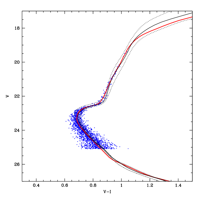
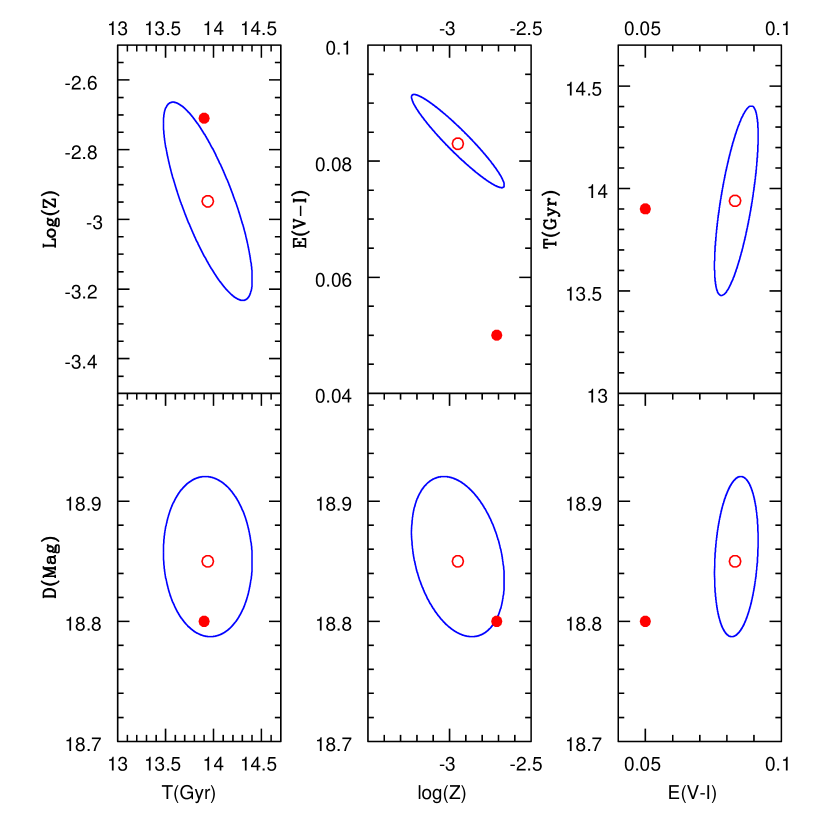
Figure 1: (Left) Simulated Single Stellar Population CMD having an age of 13.9 Gyr and $\log Z=-2.7$. The thick (black) curve shows the input isochrone, with the optimal fit isochrone recovered by the method appearing as a thin (red) curve. Dotted curves show the youngest and oldest isochrones allowed by the method, at the $1-\sigma$ level, which in fact span a 1.0 Gyr interval. (Right) The six panels show the projection of the error ellipsoid resulting from the Monte Carlo simulation and inversion of a SSP with age 13.9 Gyr and metallicity $\log Z=-2.7$, onto different planes. The filled circles show input parameters, and the empty ones the average values for the recovered parameters.

We shall refer to $G_{i}(T,Z,D,R)$ as the likelihood matrix, since each element represents the probability that a given star, $i$, was actually formed with metallicity $Z$, at time $T$ with any mass, and that it was observed with a distance modulus of $D$, and reddening of $R$. That is, in this Bayesian approach, we treat the stellar mass $m$ as a nuisance parameter which we marginalize over.

The probability that an entire observed CMD with $N_{\star}$ stars arose from a particular model, i.e., from a particular choice of parameters $(T,Z,D,R)$, will now be given by:

$${\cal L}(T,Z,D,R)\;=\;\prod_{i=1}^{N_{\star}}G_{i}(T,Z,D,R)\qquad.$$ (7)

In this way, we have constructed an optimal merit function which can be evaluated at any point within the relevant four dimensional parameter space $(T,Z,D,R)$, given an observed CMD. It is important to remark that this merit function uses all information available in the CMD densely. No binning or averaging over discrete regions is necessary, and no aspects of the distribution of stars on the CMD are discarded. Also, all the rich stellar evolutionary physics is included in the comparison with the models, as the isochrones are not being reduced to a discrete set of numbers (e.g. the position of the TO, RGB slope, etc.) or even curves on the CMD. As we shall see in section §3, the full use of all features in both data and models, allows a precise estimation of the inferred parameters.

Following Bayes theorem, one would now want to identify that point which maximizes $\mathcal{L}$, the 4 coordinates which maximize the probability that the observed CMD did in fact arise from a particular point in the parameter space, with the set of physical cluster parameters which have the highest probability of having given rise to the observed CMD.

Several methods exist for identifying the global maximum of a multi dimensional surface. Most standard methods run into considerable difficulties in cases where local maxima exist, as our problem turns out to have. The most reliable way of solving this problem is to evaluate $\mathcal{L}$  throughout a dense grid in all of the available parameter space. This however, is highly time consuming, and hence it is highly desirable to find a more efficient method.

We have used the genetic algorithm approach, where a number of “agents” are placed at random points within our parameter space, and the position of each codified into a binary number, the “genes” of each agent. The number of binary bits used for each coordinate fixes the resolution of the algorithm, which in this case corresponds to the resolution of the isochrone grid on the ($T,Z$) plane, and to 0.01 mag in the ($D,R$) plane. The value of $\mathcal{L}$ is then evaluated at the position of each agent, and the result is used as a fitness function. A second generation is then constructed by “mating” the original agents, pairing them and combining the “genes” of each parent to produce two “offsprings”. The fitness function is used to weight the mating probability, such that the fitter individuals have a greater probability of “mating”. The “genes” of the offsprings are a combination of those of their parents, and hence as generations proceed, the population gradually moves into regions where the fitness function is higher, i.e., into regions of high $\mathcal{L}$. To avoid getting trapped into local maxima, a slight “mutation rate” is introduced, through which some of the offsprings in each generation have a randomly selected “gene” switched from “1” to “0”, or vice-versa. This simplistic algorithm has been shown to converge remarkably efficiently into the global maximum of complex multi-dimensional surfaces, associated to very different problems. A more complete description of the algorithm can be found in Charbonneau (1995), with successful applications to diverse astrophysical problems being described in e.g. Teriaca et. al (1999) for fitting radiative transfer models to solar atmosphere data, Sevenster et al. (1999) in fitting parameters of Galactic structure models to observations, Metcalfe (2003), for the fitting of white dwarf astroseismology parameters or Georgiev & Hernandez (2005) in the problem of inferring optimal wind parameters from observed spectral line profiles, among many others.

3 Testing the method

In this section we test the method described in Section §2, through the inversion of a series of synthetic CMDs. As in this case the point in parameter space from which a particular CMD was simulated is known, we can optimally asses the performance of the method.

In simulating an observed CMD the first step is to obtain an adequate isochrone library. Different groups have succeeded in producing state-of-the-art stellar evolutionary codes using mostly, but not all the time, the same input physics. Since systematic errors will be produced by the choice of the set of isochrones, we use the results of the three different groups (Bergbusch & VandenBerg 1997, VandenBerg et al. 2006, Demarque et al. 2004, Girardi et al. 2002). We have worked directly with the output of stellar evolutionary codes to produce our own isochrone grid with a dense grid including 180 time steps and 120 metallicity intervals. Each isochrone contains approximately 300 stellar masses. The time resolution for ages of between 4.5 Gyr and the upper limit of 18.0 Gyr is of 0.2 Gyr, with younger ages being sampled more densely. The spacing in metallicity is linear in the logarithm, with 0.03 dex per interval. Throughout the paper we shall identify metallicity with [Fe/H], when using theoretical isochrones, or comparing against empirical inferences. The spacings of the isochrone grid will determine the maximum resolution of the method, independently of what approach is taken at the following levels of the problem. For the purposes of presenting the method, these grids are more than appropriate.

It is important to note that the highly non-linear variations in magnitude and colour with mass which appear along isochrones on critical regions of the CMD implies that a direct interpolation between two isochrones will not produce the intermediary one, but an average curve which bares little resemblance to the output of a stellar evolutionary code. In all cases, we have limited the isochrones to below the helium flash. This condition restricts the information we consider in our method to the region where disagreement between different groups working in the field is at a minimum.

Once the isochrones have been established, an IMF is chosen to distribute stars amongst different masses. This function proves to be relatively unimportant, as the mass range of stars one is dealing with is small provided stars are selected from one magnitude or so below the TO region all the way to the tip of the RGB. This ensures that the mass range probed by the observations is small. For example, in globular clusters older than $\sim 5$ Gyr the mass interval is around $1M_{\odot}$ and hence in this narrow mass range the details of the IMF are irrelevant. The distribution of stars along the isochrone is a much more sensitive function of the stellar evolutionary models, which is in fact what determines that the main sequence is highly populated, the red giant branch much more sparsely so, and that the HR gap region will contain very few stars. The IMF we use is that of Kroupa et al. (1993), although as mentioned above, any other approximation to this function would yield the same results (see §4.1).

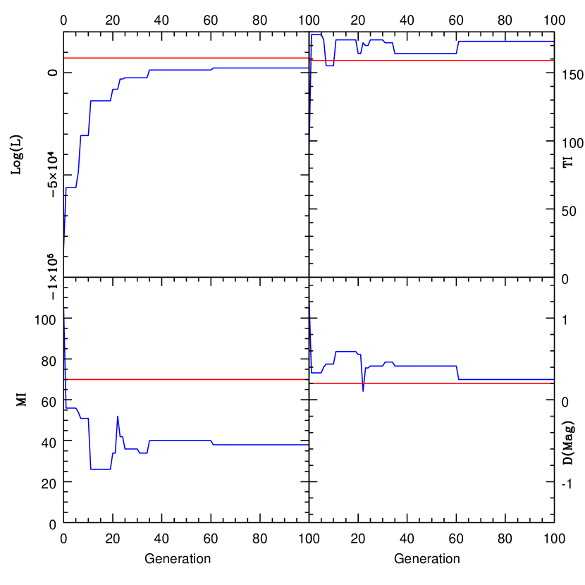
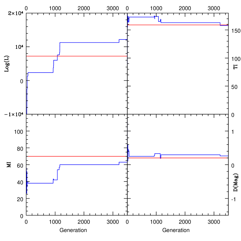
Figure 2: (Left) The four panels show, in a clockwise progression starting at the upper left, the maximum likelihood point found by the method, the optimal time index, the optimal distance modulus, and the optimal metallicity index, all as functions of generation number for the genetic algorithm simulation, for the first 100 generations. (Right) Same as the left panels, but showing the full 3500 generations of the genetic algorithm simulation.

Having an isochrone grid and an IMF, we can now pick a point in our $(T,Z,D,R)$ parameter space and place a chosen number of stars into the magnitude-colour plane. For the first implementation we have simulated an extreme example with close to 2000 stars around point $(13.9,-2.7,18.8,0.05)$, a single stellar population of age 13.9 Gyr, metallicity $-$2.7 (that is, close to $-$1.0 in solar units, for a solar metallicity of $\log Z_{\sun}=-$1.7), with a distance modulus of 18.8 magnitudes, and observed through a reddening of 0.05 magnitudes. Next we model magnitude and colour errors as Gaussian with sigmas as appropriate for current HST or high quality long integration ground-based observations. Explicitly we used

$$\sigma(L)=0.001\times\exp\left[(L+D-17.0)/2.25\right]$$

$$\sigma(C)=0.001\times\exp\left[(L+D-17.0)/1.97\right]$$

where $L$ is the magnitude, in the $V$ band, of the theoretical star, and $C$ its $V-I$ colour. At this point we can now produce a synthetic CMD, and for this first test obtain the 2009 points shown in Figure 1. A magnitude cut at $V=25$ has been used, limiting analysis to stars brighter than this cutoff. Given the highly correlated way in which star populate the main sequence, together with growing and sometimes divergent errors towards higher magnitudes, it is sufficient to restrict analysis to 2 magnitudes below the ’turn off’ region. In what follows we shall keep the 25 magnitude lower limit, although a changing magnitude cut as described above yields the same results.

At this point, Equation 7 can be used to obtain the likelihood function of the simulated CMD with respect to any given point on our 4-D parameter space. As discussed in section §2, the seeking of the optimal point will be carried out through a genetic algorithm simulation, the workings of which, for this first example, we describe below.

The upper left panel of Figure 2 shows the evolution of the value of the likelihood merit function of Equation 7 over the first 100 generations of the genetic simulation. The horizontal line gives the value of this same function, evaluated at the actual point in our $(T,Z,D,R)$ parameter space which was used to produce the synthetic CMD being inverted. This first panel shows an increase with the generation number of the optimal value of the likelihood function, as the absolute best point found in all the simulation up to a given generation is what is being plotted. This value increases very rapidly at first, as the initially random points begin to migrate towards regions more closely resembling the simulated CMD, but progress becomes increasingly slower. In fact, there is no definitive criterion to establish when a genetic algorithm simulation has finally converged, this has to be inferred from simulations with synthetic data and repeated experiments, as an approximate number of generations, suitable for a particular problem, after which no further improvement is achieved. For the problem being treated here, we have found the method stops yielding any improvement in the fits in general well before 3500 generations. We have thus ended the genetic simulations at 3500 generations. The value of the likelihood function evaluated at the actual input point always remains above the one corresponding to the optimal one found by the simulation for this first 100 generations shown here.

The upper right panel of Figure 2 gives the evolution of the optimal time grid index (TI) along the isochrone grid, found up to a certain point. In this case, the input age of 13.9 Gyr corresponds to our time index 159 out of 180, over this initial 100 generation period the time index corresponding to the optimal model found fluctuates from an initial value of 120 to 178, from 6 to 18 Gyr, and ends this initial period 12 grid points above the input value, at 16.9 Gyr. The bottom left and right panels show the corresponding evolution of the metallicity index and the distance modulus, again, the horizontal line gives the input parameters. We can see that after 2 generations the initially random values have approached significantly the input ones, and then show considerable variations of around 35 metallicity grid intervals (1.5 dex) and 0.8 mag in the distance modulus.

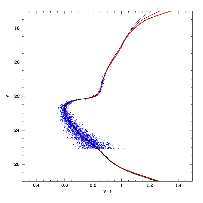
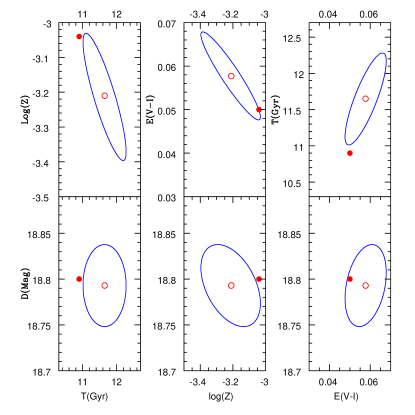
Figure 3: (Left) Simulated Single Stellar Population CMD having an age of 10.9 Gyr and $\log Z=-3.05$. The thick (black) curve shows the input isochrone, with the optimal fit isochrone recovered by the method appearing as a thin (red) curve. Dotted curves show the youngest and oldest isochrones allowed by the method, at the $1\sigma$ level, which in fact span a 1.48 Gyr interval. (Right) The six panels show the projection of the error ellipsoid resulting from the Monte Carlo simulation and inversion of a single stellar population with age 10.9 Gyr and metallicity $\log Z=-3.05$, onto different planes. The filled circles show input parameters, and the empty ones the average values for the recovered parameters.

It is interesting to re-plot the left panel of Figure 2 this time over the entire 3500 generation range, this is done in the right panel of Figure 2 where we can see that substantial improvements in the optimal likelihood value found are still occurring after 1000 generations. A striking feature seen in the upper left panel of this last Figure is that the genetic algorithm has actually found an optimal model which in fact yields a likelihood value above that of the input parameters. At around 1000 generations, the optimal likelihood found crosses the horizontal line giving the likelihood value of Equation 7 of the input parameters, with respect to this particular realization of the CMD corresponding to them. This apparently paradoxical result is in fact unavoidable, and highlights the statistical nature of the problem. The construction of a CMD from a point in the single stellar population parameter space can not be thought of as neither a deterministic nor a unique process. Even before the errors associated with procuring the observations enter the picture, the process of sampling an IMF has already introduced a probabilistic ingredient intrinsic to the cluster itself (e.g. Cerviño et al. 2002, Cerviño & Valls-Gabaud 2003). In this sense, obtaining a single simulated CMD and using it to compare with an observed one can only be at best a crude first approximation to the inverting of a CMD. In this particular case, the convolving of the theoretical stars with error gaussians has shifted the points around in such a way that the isochrone (understood as a series of stellar evolutionary models, not just a curve on a CMD) which has the greatest probability of having yielded the CMD is not the input one, but one which is one time grid interval above (0.2 Gyr), 11 metallicity grid intervals below (0.4 dex) and at a distance modulus around 0.05 magnitudes larger than the input parameters.

The above result makes it clear that inferring structural parameters of stellar populations, even in the simplest cases, can not be attempted without a full consideration of the probabilistic nature of the problem, and also, can not give error-free results. However, it is possible to evaluate the intrinsic errors of the method, in connection to any particular implementation, by the Monte Carlo method. The experiment is repeated a large number of times, and the various answers analyzed to obtain mean inferred values with well determined dispersions and correlations.

This method naturally takes into consideration all internal sources of error and dispersion inherent to the procedure being tested, and yields accurate and reliable confidence intervals on the inferences obtained. Figure 1 (right) shows with filled circles the input parameters of the CMD of Figure 1 and with empty ones the center of the distributions of the recovered parameters after the whole procedure of constructing a synthetic CMD and inverting it was repeated 20 times. The ellipses give projections of the error ellipsoid onto the different planes being shown. It can be seen that the only systematic which appears in this case beyond the $1\sigma$ level is an $+$0.03 magnitude offset in the recovered values of the reddening for the cluster. All other parameters have been recovered with no systematics, the $1\sigma$ errors for this 13.9 Gyr old cluster being 0.5 Gyr in age, 0.38 dex in metallicity and 0.05 mag in the distance modulus.

The isochrone corresponding to the solid circles is shown in Figure 1 by the thick solid curve, which practically lies above the thin (red) curve of the isochrone corresponding to the empty circles along all the CMD. Some differences between the two isochrones are evident along the upper half of the red giant branch, where so few stars are expected, that none of the 2009 obtained in the CMD realization shown appear there. The dotted curves give the isochrones corresponding to the oldest and youngest points on the ellipse in the age-metallicity plane, which are seen to bracket the HR-gap and RGB regions of the CMD shown.

The second example was constructed from point $(10.9,-3.05,18.8,0.05)$ in our parameter space, taken to represent a typical old Single Stellar Population (SSP). In testing the method for systematics related to effects not explicitly included in the model, comparisons will be made at this point in parameter space, in section § 4.

Figure 3 shows the CMD which results from convolving the modeled stars with the same simulated errors than last time. Also shown are the isochrone from which the simulated stars were constructed, thick (black) curve, and the optimal one found by the genetic algorithm, thin continuous curve. The dotted curves give the oldest and youngest isochrones consistent with the Monte Carlo simulation on the inverting procedure at a $1\sigma$ level, this time spanning 1.2 Gyr. Analogous to Figure 1, Figure 3(right) gives the projection of the error ellipsoid for the inferred parameters using the Monte Carlo method, projected onto 6 different planes. One again sees that there are no systematics beyond the $1\sigma$ level, from which we conclude that the method accurately recovers the input parameters of the cluster, and yields meaningful confidence intervals for the answer supplied.

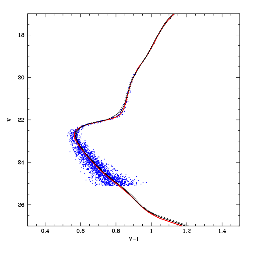
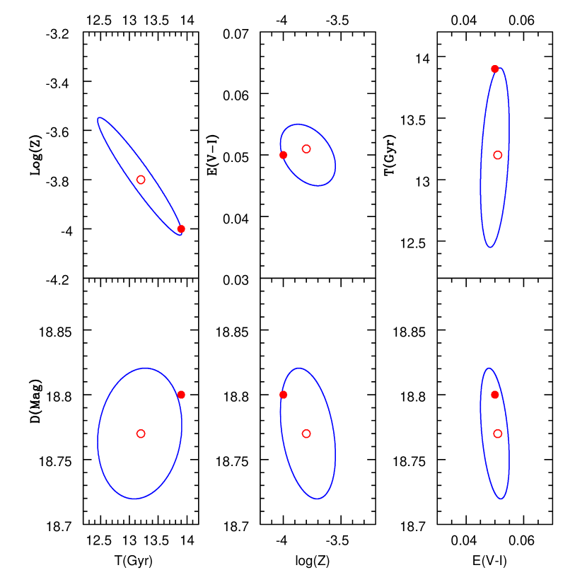
Figure 4: (Left) Simulated Single Stellar Population (SSP) CMD having an age of 13.9 Gyr and $\log Z=-4.0$. The thick (black) curve shows the input isochrone, with the optimal fit isochrone recovered by the method appearing as a thin (red) curve. Dotted curves show the youngest and oldest isochrones allowed by the method, at the $1\sigma$ level, which in fact span a 1.44 Gyr interval. (Right) The six panels show the projection of the error ellipsoid resulting from the Monte Carlo simulation and inversion of a SSP with age 13.9 Gyr and metallicity $\log Z=-4.0$, onto different planes. The filled circles show input parameters, and the empty ones the average values for the recovered parameters.

Looking at the upper left panel of Figure 3 (right) we clearly see the actual intrinsic age-metallicity degeneracy in the way the $1\sigma$ ellipse in the ($T,Z$) plane slants from the upper left to the lower right. Optimal fits with large ages tend to correspond to lower metallicities, and vice-versa. However, we see that having included all the information available both in the simulated CMD and in the theoretical isochrones minimizes this degeneracy and one obtains closed confidence intervals. If the CMD is reduced to, say two numbers, corresponding to the location of the ’turn off’, when comparing to a similarly restrictive view of what the stellar evolutionary models encode, one ends up with a confidence region which spans an extensive region of the ($T,Z$) plane, merely a relation between the possible age and metallicity, with no way of restricting the answer to a narrower region. The above highlights problems inherent to methods where information is being discarded, to which must be added ambiguities associated to the definition of the ’turn off’ point. Given the current high accuracy of the observations and the theoretical isochrones, inspection of simulated and observed CMDs makes it clear that there is in fact no such thing as a turn off ’point’, but rather a diffuse, hazy region which is prone to sampling fluctuations and the presence, or otherwise, of a few odd stars.

Other correlations are evident in Figures 1 and 3, for example a clear negative correlation between the inferred reddening and metallicity, also a generic feature of any stellar population inversion method, inherent to the structure of the isochrones. It is interesting to note in the lower 3 panels of Figures 1 and 3 that the inferred distance to the cluster shows no strong correlations with any of the other 3 parameters, contrary to what happens when the isochrones are reduced to a set of numbers such as location of the turn off point, slope of the RGB etc.

For a third example, in trying to cover points on our parameter space representative of old SSPs, we simulated an old, metal poor such system. Starting from point $(13.9,-4.0,18.8,0.05)$ we construct a series of CMDs, one of which is shown in Figure 4, with curves analogous to what appears in Figures 2 and 3. It is impressive to see how nearly indistinguishable the shapes of the input and mean recovered isochrones are on the CMD, together with the isochrones corresponding to the oldest and youngest isochrone allowed by the Monte Carlo simulation at a $1\sigma$ level. All 4 of these curves appear practically on top of each other in this case, with very minor differences only apparent at the curvature between the HR gap region and the RGB.

The above is particularly surprising when considering that the isochrones shown span almost a 1.5 Gyr-long time interval. Of course, the other parameters besides the age have been adjusted to maximize the fit when shifting the age, in accordance with the correlations shown in Figure 4, the oldest isochrone has the lowest metallicity together with a somewhat above average reddening correction. This point again shows that the isochrones have to be treated as collections of full stellar evolution models, not reduced to a few scalar shape parameters, not even to simply shapes on the CMD. Having used the full shape of the isochrones continuously throughout the full CMD, together with information regarding the duration of different stellar phases in constructing the merit function of Equation 7 has allowed a much finer discrimination within our $(T,Z,D,R)$ parameter space, much beyond what considering only the shape of the isochrones would have allowed. Changing the input parameters of the isochrone even at a 2-3 sigma level, would result in curves compatible with the shape of the simulated stellar distribution, but which are ruled out due to having included all available information both in the CMD and the stellar models.

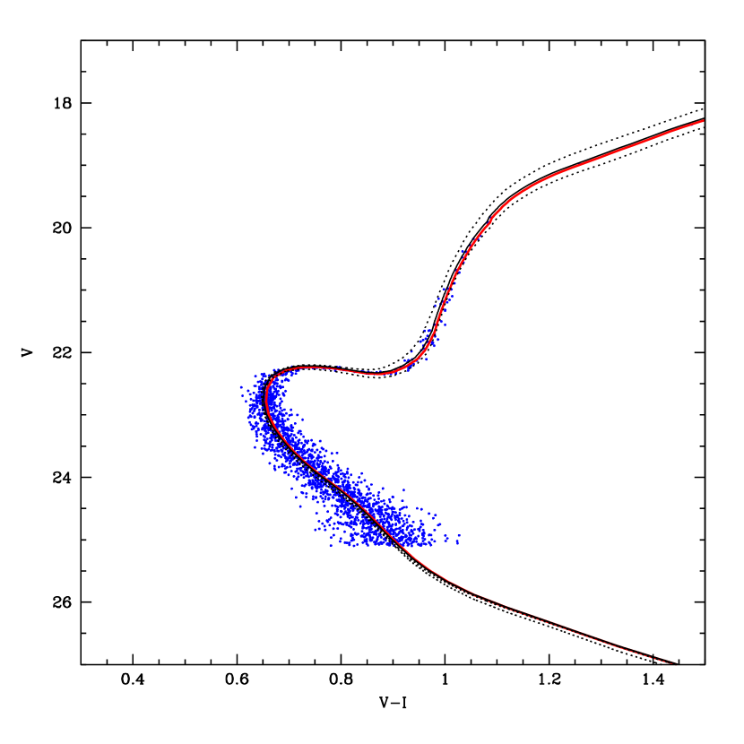
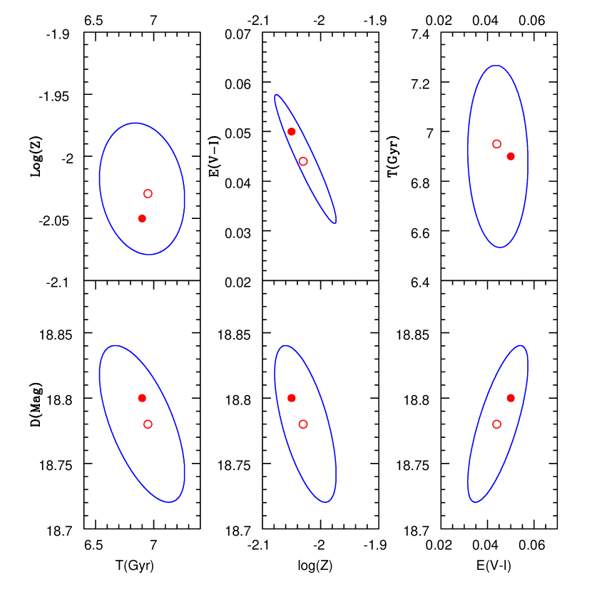
Figure 5: (Left) Simulated Single Stellar Population CMD having an age of 6.9 Gyr and $\log Z=-2.05$. The thick (black) curve shows the input isochrone, with the optimal fit isochrone recovered by the method appearing as a thin (red) curve. Dotted curves show the youngest and oldest isochrones allowed by the method, at the $1\sigma$ level, which in fact span a 1.0 Gyr interval. (Right) The six panels show the projection of the error ellipsoid resulting from the Monte Carlo simulation and inversion of a SSP with age 6.9 Gyr and metallicity $\log Z=-2.05$, onto different planes. The filled circles show input parameters, and the empty ones the average values for the recovered parameters.

Again, no systematic offsets between the input values and the mean recovered ones appears beyond the $1\sigma$ level, as can be seen from Figure 4. In this same Figure we see the same correlations evident in the previous analogous Figures, with the confidence intervals, particularly in age and metallicity having grown considerably in comparison to Figure 3. This is obvious when one considers how consecutive isochrones equally spaced in time will show progressively smaller differences as the age of a stellar population increases. Having left the assumed observational errors and stellar numbers constant, the uncertainties in the inferred parameters have grown in going to an old, metal poor population.

For the fourth and fifth examples we complete our sampling of SSPs parameter space with two clusters at $(6.9,-2.0,18.8,0.05)$ and $(6.9,-3.37,18.8,0.05)$. Figures 5 and 6 are completely analogous to the corresponding previous figures and essentially illustrate the same points mentioned before. For these younger simulated stellar populations the mean recovered parameters appear within one grid interval in metallicity of the input parameters, the theoretical maximum resolution of the implementation has been realized at these young ages, even after having considered realistic errors in magnitudes and colours. The age resolution is still above that of the isochrones, but robust $1\sigma$ errors of around 0.5 Gyr are encouraging.

We add that the precision of the method in recovering distance modulus and reddening parameters is sufficient to make it a useful tool in the determination of distances to single stellar populations, with errors sometimes as good as a few hundredths of a magnitude, as seen in Figure 5. Again, the correlations persist, although the details of these correlations change from example to example in ways that reflect the details of the isochrones around each region, and which are dependent on both the magnitude of the assumed observational errors and the actual numbers of stars present in the simulated CMDs.

With simulated errors tending to zero the inferred parameters would tend to the input ones, to within the resolution of the isochrone grid used, always. Also, if the statistical comparison between data and models is robust, the systematics and confidence intervals should tend to zero as the number of data points tends to infinity, which of course is never the case.

4 Systematics

Having tested successfully the method across representative points in the $(T,Z,D,R)$ space, we now turn to the problem of estimating how robust the inferences of our method will be in more realistic cases, where physical ingredients not explicitly considered in the statistical modeling behind Equation 7, and present in a real application, will complicate matters, and might result in systematic offsets between the actual physical parameters of a stellar population and our inferences.

In this section we explore such cases by constructing synthetic CMDs under assumptions different to the ones the method uses in the inversion procedure, and compare how serious these effects are in altering our inferences. The 5 effects considered will be: (1) Errors in the assumed IMF, (2) the presence of unresolved binaries, (3) the effects of reducing the numbers of stars present in the observed CMD, (4) systematics associated with the different sets of stellar tracks used in constructing the isochrone grids, and (5) the presence of contaminating stars in the observed CMDs.

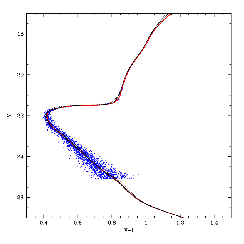
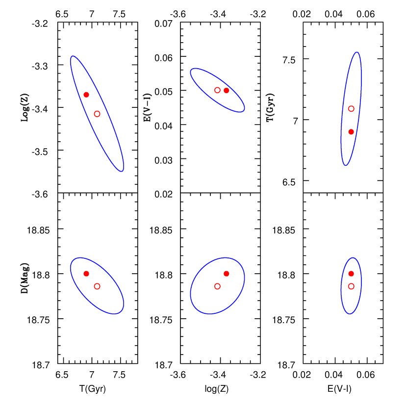
Figure 6: (Left) Simulated Single Stellar Population CMD having an age of 6.9 Gyr and $\log Z=-3.37$. The thick (black) curve shows the input isochrone, with the optimal fit isochrone recovered by the method appearing as a thin (red) curve. Dotted curves show the youngest and oldest isochrones allowed by the method, at a $1\sigma$ level, which in fact span a 1.0 Gyr interval. (Right) The six panels show the projection of the error ellipsoid resulting from the Monte Carlo simulation and inversion of a SSP with age 6.9 Gyr and metallicity $\log Z=-3.37$, onto different planes. The filled circles show input parameters, and the empty ones the average values for the recovered parameters.

4.1 Effects of the IMF

Figure 7 gives a CMD resulting from the same point in parameter space as Figure 3, $(10.9,-3.05,18.8,0.05)$, but created this time using a substantially different IMF, heavily weighted towards massive stars, increasing the slope with respect to the Kroupa et al. (1993) IMF such that the typical stellar mass increases by a factor of 3. Obtaining the same number of points thus requires turning a much larger total mass into stars, but under the assumption of an equal number of stars as in Figure 3, the results are highly similar. The precise manner in which the density of stars varies along the main sequence region is somewhat different from the case of Figure 3, but given the highly correlated manner in which magnitudes and colours scale along this region, the information content of the CMD is only marginally altered. The highly determinant sections beyond the main sequence span such a small mass range that all of these features are virtually left unchanged by even the strongest modifications in the IMF.

The inversion procedure was repeated 20 times, but assuming the same IMF as in Figure 3, which in this case no longer corresponded to the IMF used to create the synthetic CMDs. The results of the Monte Carlo procedure can be seen in Figure 7, which from the previous discussions would not have been expected to show any substantial difference to Figure 3, as is indeed the case. By comparing with Figure 3 we note no substantial differences, all inferred parameters are well within the $1\sigma$ error estimates, with very low uncertainties of around 0.5 Gyr in age, 0.2 dex in metallicity, 0.01 and 0.05 mag in reddening and distance modulus, respectively. The isochrones corresponding to the input, inferred, and oldest and youngest values recovered (at a $1\sigma$ level), practically overlap over the entire region over which significant numbers of stars are found. We see that the theoretical expectations of the previous sections are borne out, and our results are in fact highly robust to even large scale features of the IMF. This is reassuring from the point of view of inferring ages, metallicities, distances and reddening corrections of resolved stellar populations, but disheartening from that of inferring the IMF of observed stellar clusters through methods similar to what has been developed here.

4.2 Effects of unresolved binary stars

The second test was performed again using the same isochrone library, and the input point $(10.9,-3.05,18.8,0.05)$ of Figure 3, but this time to one in two of the simulated stars we added an unresolved companion, chosen from the same IMF, i.e., the synthetic CMD was produced assuming a 50% unresolved binary contribution. The inversion procedure was however exactly the same as in the previous cases, with Equation 7 remaining unchanged, a binary fraction of 0% was assumed in recovering the inferred parameters.

One of the resulting CMDs which was used in the Monte Carlo procedure for the inversion is shown in Figure 8, together with isochrones as in the previous Figures. The presence of 50% binaries is particularly conspicuous along the main sequence, where the distribution of points is clearly smeared towards redder colours, evident when comparing, for example, with Figure 7. A few binaries can also be seen around the critical turn off region, but these have had little effect. Given the large difference in luminosity between a RGB star and any main sequence one (the most likely secondary to be added to a binary), binary pollution along the RGB produces absolutely no effects.

By looking at the best fit inferred isochrones at the base of the main sequence, it can be seen that these have all shifted towards the right, in response to the weighting of the distribution of points towards this direction. By looking at Figure 8 one can see that this shift towards the right has been achieved optimally by the genetic algorithm not by altering the reddening correction, but rather through an offset in the distance modulus. Whilst inferred age, metallicity and reddening parameters have been obtained within the $1\sigma$ error ellipses, the inferred distance modulus is off at around a $2\sigma$ level, which however corresponds only to 0.15 magnitudes. The clearest correlation between the inferred parameters is still in the age-metallicity plane, and remains in the same sense as expected.

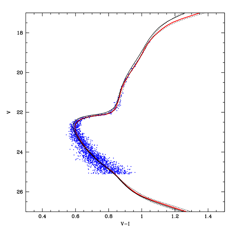
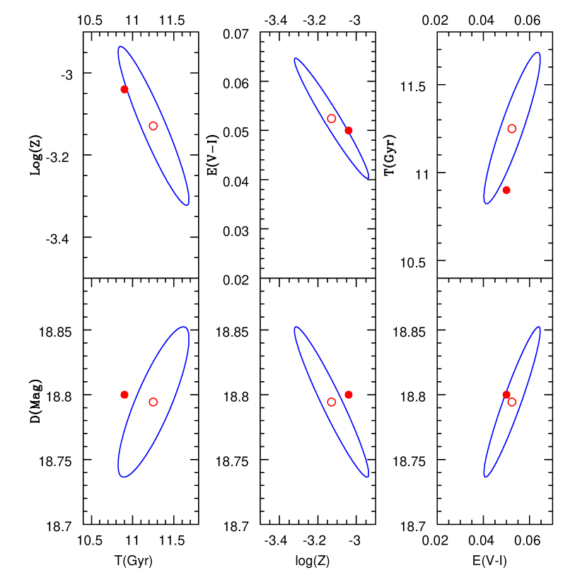
Figure 7: (Left) Simulated Single Stellar Population CMD having an age of 10.9 Gyr and $\log Z=-3.05$. The thick (black) curve shows the input isochrone which was used assuming a high mass weighted IMF, with the optimal fit isochrone recovered by the method, assuming the standard IMF, appearing as a thin (red) curve. Dotted curves show the youngest and oldest isochrones allowed by the method, at the $1\sigma$ level, which in fact span a 0.9 Gyr interval. (Right) The six panels show the projection of the error ellipsoid resulting from the Monte Carlo simulation and inversion of a SSP with age 10.9 Gyr and metallicity $\log Z=-3.05$, onto different planes, for CMDs constructed using a high mass weighted IMF and inverted using the standard IMF. The filled circles show input parameters, and the empty ones the average values for the recovered parameters.

Other than the slight offset in inferred distance modulus, the only other effect of having introduced a relatively high binary population has been the broadening of the errors. The confidence region is this time 2.5 Gyr across, compared to 1.4 Gyr for Figure 3. Again, the isochrones in Figure 8 are remarkably close to each other, but although regions beyond the turn off have not been much affected by the inclusion of the binaries, the fact that the main sequence has shifted out of correspondence with these other regions has resulted in poorer fits, and although no systematic offsets in age, metallicity or reddening correction have appeared, the error ellipses have certainly increased in size.

The particular case of blue stragglers has not been treated, but a good approximation can be obtained from the binary contamination example included. Binaries and blue stragglers can populate the region close to the turn off, and result in poorer fits. However, having weighted all the CMD equally, the much larger main sequence population, and the phases beyond the turn off, where errors are much smaller, anchor to a large extent the fit against a small number of blue stragglers or binaries very close to the turn off. More than 2 local error sigma away from the turn off, you can fill in almost any number of blue stragglers, by construction their effect will be negligible, see Eq. 4.

In the context of inverting resolved stellar populations, a binary does not necessarily imply a physical gravitational association between two stars, but merely that the light of two individual stars has appeared in the data as coming from a single point. The two stars hence show as a single one having the total luminosity of the sum for the two stars, and an effective temperature being the energy weighted sum of the temperatures of the two stars, as per a Stefan-Boltzmann law. Therefore, especially if thinking of dense systems such as globular clusters where crowding effects can be dominant, the adoption of the same IMF for the secondary component of the binary as for the primary one is justified.

4.3 Effects of different sets of isochrones

We now turn to a possibly important systematic, related to the validity of the underlying hypothesis that a single real star from an observed CMD does in fact behave and evolve as the stellar evolutionary code one is using to construct an isochrone grid assumes it to. Figure 9 gives the CMD produced again from the same point $(10.9,-3.05,18.8,0.05)$ in parameter space, but using this time the Padova stellar evolutionary models (Girardi et al. 2002), whilst in all previous examples, the Yale isochrones where used (Demarque et al. 2004). The distribution of stars on the magnitude-colour plane is much the same as in Figure 3, and no significant differences can be detected.

A number of such CMDs where then inverted using the Yale isochrones, resulting in the error ellipsoid whose projections onto the 6 usual planes is shown in Figure 9. The most immediate conclusion is that changing the stellar models has resulted in no systematics beyond the $1\sigma$ level, beyond a slight offset in the recovered reddening correction of around 0.02 magnitudes. Asides from the above, comparing with Figure 3 we note that using a ’wrong’ isochrone grid in the inversion procedure has resulted in slightly poorer fits, evident in larger error bars on the recovered parameters, the extremes of the $1\sigma$ confidence interval now span close to 2.0 Gyr, as opposed to only 1.2 Gyr when the same isochrone set was used to construct the CMDs and to invert them. This has been due to the details of the stellar evolutionary code in terms of the differential duration of stellar phases, more than to changes in the isochrones as plotted on the CMDs. In this particular case, the error ranges for the metallicity have grown by a larger fraction than the others. However, this is not a general feature of changing the isochrone set, but something which depends on the errors, no. of stars considered, actual age, distance and metallicity of the SSP being studied. Regarding the error ranges, the examples we have shown are only illustrative, and trustworthy error ranges have to be internally calculated for each particular case.

Note also that these different sets of isochrones use different calibrations to go from the theoretical diagram to the observed ones in the different sets of filters. This is perhaps the largest source of uncertainty at this level (VandenBerg 2007) for this range of masses and ages.

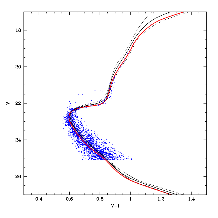
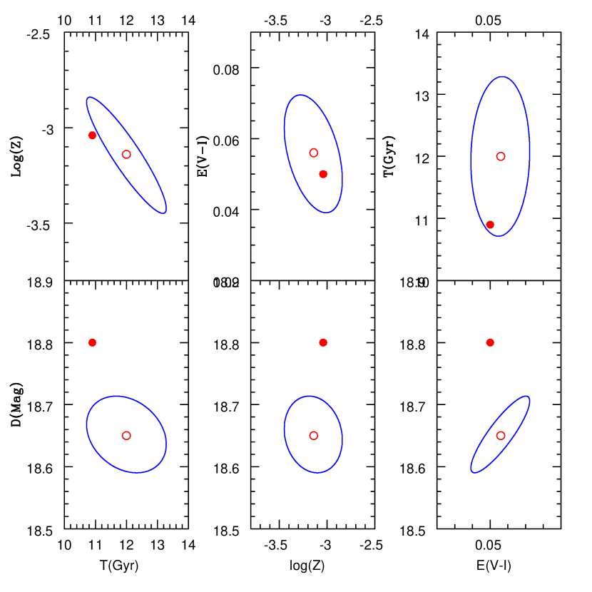
Figure 8: (Left) Simulated Single Stellar Population CMD having an age of 10.9 Gyr and $\log Z=-3.05$. The thick (black) curve shows the input isochrone which was used adding an unresolved binary companion to 50% of the stars, with the optimal fit isochrone recovered by the method, assuming no binaries, appearing as a thin (red) curve. Dotted curves show the youngest and oldest isochrones allowed by the method, at the $1\sigma$ level, which in fact span a 1.52 Gyr interval. (Right) The six panels show the projection of the error ellipsoid resulting from the Monte Carlo simulation and inversion of a SSP with age 10.9 Gyr and metallicity $\log Z=-3.05$, onto different planes, for CMDs constructed including 50% unresolved binaries and inverted assuming no binaries. The filled circles show input parameters, and the empty ones the average values for the recovered parameters.

All the isochrones throughout have been used only up to the tip of the RGB, with regions beyond which give rise to interesting ’red clump’ morphologies, having been excluded from the analysis. Even though inclusion of these phases, for example the HB region, would provide interesting independent restrictions and potentially enhance the effectiveness of the method, at present post helium flash regions have to be modeled through the inclusion of RGB mass loss rate recipes which can not yet be calculated or constrained from first principles. Thus, their inclusion would necessarily imply obtaining inferences which would be limited to the validity of the currently poorly grounded hypotheses one would chose regarding late stellar evolution.

Perhaps we can not conclude that stellar evolutionary modeling has converged to a final solution, even below the helium flash. However, by using broad band colours, where integration over relatively wide sections of a stellar spectrum is included, an averaging over details in fine features, and by restricting the analysis to stellar phases which are well understood, a method such as what we have implemented here is now capable of yielding results which are highly robust with regards to the current discussions and disagreements over stellar evolution.

Certainly in going from Figure 3 to Figure 9 the error ranges have increased, but the inferences correctly identify ages, metallicities and distances to within internally computed confidence intervals. In future, it would be desirable to use stellar evolutionary models more extensively, including phases beyond the helium flash, to yield much more restrictive inferences and narrow error ranges, but whilst debate rages over the physics of stars in those regions, we prefer to increase the size of both our error ranges and our confidence in the final results. The same applies to the use of more detailed features of stellar spectra, in going from broad band colours to narrow band colours and finally details of the emission line structure, more information is encoded, the potential of more refined inferences is there, but at least until the different models converge, inferences using such details should be considered as subject to short term revision.

4.4 Sampling and background/foreground contamination

As remarked previously, the numbers of stars in an observed CMD and the size of the observational errors dispersing the stars from their intrinsic locations all influence the quality of the inferences which can be obtained. Figure 10 is analogous to Figure 3, the same point in parameter space has been modeled, with the same errors, but the number of stars has been reduced in half, of the $\sim 2000$ stars simulated in all previous examples, only $\sim 1000$ where simulated this time.

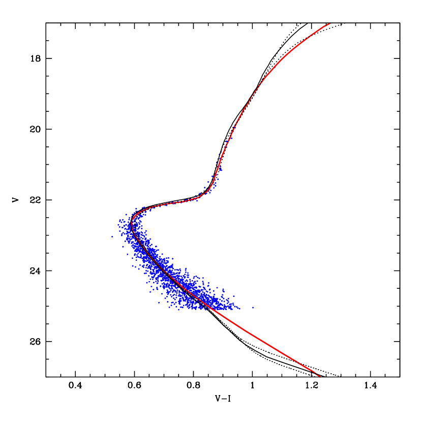
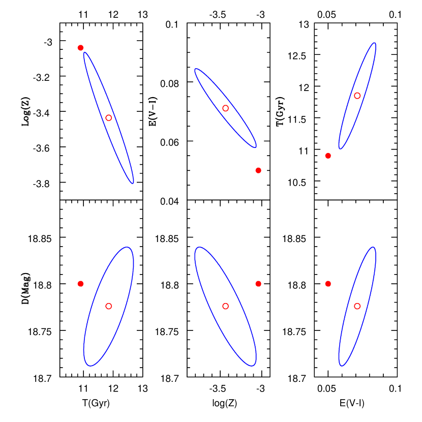
Figure 9: (Left) Simulated Single Stellar Population CMD having an age of 10.9 Gyr and $\log Z=-3.05$. The thick (black) curve shows the input isochrone (Padova models), with the optimal fit isochrone (Yale models) recovered by the method, appearing as a thin (red) curve. Dotted curves show the youngest and oldest isochrones allowed by the method, at a $1\sigma$ level, which in fact span a 1.8 Gyr interval. (Right) The six panels show the projection of the error ellipsoid resulting from the Monte Carlo simulation and inversion of a SSP with age 10.9 Gyr and metallicity $\log Z=-3.05$, onto different planes, for CMDs constructed using Padova models and inverted using Yale ones. The filled circles show input parameters, and the empty ones the average values for the recovered parameters.

We see from Figure 10 that no systematics appear, and that even with only $\sim 1000$ stars, a number easily achievable in current observations of Galactic Single Stellar Populations, the recovered parameters are all within the $1\sigma$ error ellipses of the input ones. By comparing with Figure 3 we do note that again, as in the two previous experiments, the confidence intervals have grown considerably, a similar trend is seen if the assumed observational errors are increased. The CMD of Figure 10 is clearly much more thinly populated than previous ones, but still the method manages to recover isochrones that do not differ much in their parameters from the input ones.

Table 1: Summary of the systematics effects explored. The recovered (output) values include their corresponding 1$\sigma$ confidence intervals.

Test	Figure	$t$(input) (Gyr)	$t$(output) (Gyr)	$\log Z$ (input)	$\log Z$ (output)	$D$ (mag)a	$R$ (mag)b
Old metal rich SSP	1	13.90	13.95 $\pm$ 0.50	$-2.70$	$-2.95\pm 0.38$	18.845 $\pm$ 0.06	0.082 $\pm$ 0.015
Typical old SSP	3	10.90	11.65 $\pm$ 0.74	$-3.05$	$-3.21\pm 0.17$	18.795 $\pm$ 0.04	0.059 $\pm$ 0.015
Old metal poor SSP	4	13.90	13.20 $\pm$ 0.72	$-4.00$	$-3.80\pm 0.21$	18.775 $\pm$ 0.04	0.051 $\pm$ 0.008
Young metal rich SSP	5	6.90	6.950 $\pm$ 0.50	$-2.05$	$-2.03\pm 0.06$	18.780 $\pm$ 0.06	0.045 $\pm$ 0.012
Young metal poor SSP	6	6.90	7.100 $\pm$ 0.50	$-3.37$	$-3.41\pm 0.13$	18.785 $\pm$ 0.03	0.050 $\pm$ 0.006
Wrong IMF	7	10.90	11.25 $\pm$ 0.45	$-3.05$	$-3.13\pm 0.20$	18.795 $\pm$ 0.06	0.051 $\pm$ 0.012
50% binaries	8	10.90	12.00 $\pm$ 1.26	$-3.05$	$-3.15\pm 0.30$	18.650 $\pm$ 0.06	0.056 $\pm$ 0.015
Wrong isochrones	9	10.90	11.90 $\pm$ 0.90	$-3.05$	$-3.44\pm 0.38$	18.775 $\pm$ 0.06	0.070 $\pm$ 0.014
50% less stars	10	10.90	11.40 $\pm$ 1.05	$-3.05$	$-3.13\pm 0.25$	18.772 $\pm$ 0.07	0.049 $\pm$ 0.021
60% contamination	11	10.90	12.08 $\pm$ 1.39	$-3.05$	$-3.12\pm 0.41$	18.751 $\pm$ 0.12	0.061 $\pm$ 0.023

^a The input distance modulus was kept at 18.80 mag in all cases.
^b The input reddening was kept at 0.05 mag in all tests.

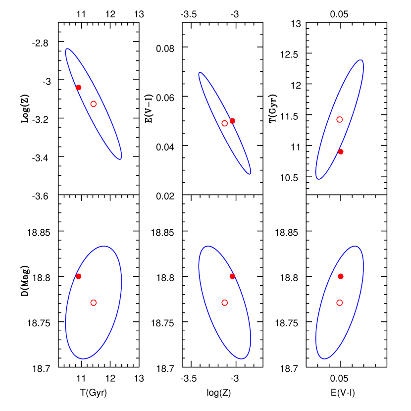
Figure 10: (Left) Simulated Single Stellar Population CMD having an age of 10.9 Gyr and $\log Z=-3.05$. The thick (black) curve shows the input isochrone, with the optimal fit isochrone recovered by the method, appearing as a thin (red) curve. Dotted curves show the youngest and oldest isochrones allowed by the method, at the $1\sigma$ level, which in fact span a 2.1 Gyr interval. (Right) The six panels show the projection of the error ellipsoid resulting from the Monte Carlo simulation and inversion of a SSP with age 10.9 Gyr and metallicity $\log Z=-3.05$, onto different planes, for CMDs constructed using only $\sim 1000$ star as opposed to the $\sim 2000$ used in all previous examples. The filled circles show input parameters, and the empty ones the average values for the recovered parameters.

As a final test of systematics which surely apply to the use of real data, we present Figure 11, where a fraction of 60% (by number) of polluting stars have been added to the CMDs, also produced from the same parameters as the previous tests. The presence of polluting stars is evident in Figure 11 where the area in the CMD which is taken into account in the analysis is clearly seen to have been filled with contaminating stars. To make this example as realistic as possible, we have modeled the contamination produced by field stars using the Besançon model of the Galaxy (Robin et al. 2003). We simulated a field of one square degree along the direction $(l,b)=(45^{\circ},23^{\circ})$ so that a significant contribution by the thin and thick discs is present. The errors which we have assumed apply to the polluting points are the same as the average for the actual ’observed’ stars at a given luminosity. From the 87000 simulated stars along that direction, we extracted a random sample of size 1200 to simulate a severe contamination of 60 % with respect to the number of stars in the CMD of the simulated cluster. This contamination appears in the CMD as an essentially constant density addition of random stars, as the typical scales over which variations appear in the Besançon model in both colour and magnitude, are larger than the domains of Figure 11.

From the integral over the model isochrone being compared to the data shown in equation 6, and from the form of $G_{i}(T,Z,D,R)$ of equation 4, it is obvious that a given star will only contribute significantly to ${\cal L}(T,Z,D,R)$ for isochrones passing within 1-2 $(\sigma(L_{i})^{2}+\sigma(C_{i})^{2})^{1/2}$ of it. The convolution of the error Gaussian which maps the model stars onto the CMD and the error Gaussian for an observed star converges quickly within a distance of $2\sigma$ of either. This means that features not yet well modeled by the theoretical stellar models, but which fall directly on the isochrones, such as the Red Giant Branch bump morphology seen in luminosity functions of RGBs, will not have any effect at all on our inferences. The CMDs we have modelled do not have sufficient stars to properly allow us to identify any Red Giant Branch bump, however, this feature is a second order effect the paucity of which, together with the fact that it does not move stars out of the isochrone, and only slightly changes the details of the density of points along it, that make the method robust against it. The uncertainties in our inferences due to the level of observational errors are already much larger than anything theoretical Red Giant Branch bump uncertainties might introduce. Similarly, the presence of a small number of blue stragglers will tend to bias the estimation, but given that their number is small in comparison with all the other stars which lie along the tentative isochrone, they do not bias the final estimate.

The above discussion leads us to expect that the method we have constructed should be highly robust against the presence of contaminating stars, as indeed can be concluded from Figure 11, where the resulting error ellipses for this experiment are shown. We can see that although the errors have increased, all inferred parameters are practically within $1\sigma$ error ellipses of the input ones. Some inferences are more affected than others, for example, the error in the age determination has nearly doubled when compared to Figure 3, but the one in the reddening correction has hardly changed. This result holds even for large polluting fractions than what is being simulated, and in fact suggests that the method can be applied to the identification of stellar populations in fields crowded by foreground and background contamination. The method is however sensitive to ’polluting’ stars occurring systematically close to critical regions of the isochrones, e.g. a sequence slightly off to one side of the RGB corresponding to the observed main sequence, essentially equivalent to having used grossly mistaken stellar tracks. The precise effect of foreground/background contamination will in fact depend on the details of the SSP being studied, $(T,Z,D,R)$ parameters, numbers of stars and observational errors, and location of contaminating stars. The final Monte Carlo assessment of the confidence intervals must hence also include a modeling of the fields contamination, in order to yield meaningful results.

Lastly, as a summary of these last 2 sections we present Table 1, where all the synthetic cases we have treated are given. The values for $(T,Z,D,R)$ in the table give the input parameters, followed by the recovered ones with the corresponding 1 sigma error ranges.

5 An example with observations

In this final section we present an example of the workings of the method, using data from an observed SSP, where in a sense, all possible systematics are at work. Of the 7263 stars observed by Rosenberg et al. (2000) for the globular cluster NGC 3201, we take the 5197 stars brighter than $V=20$, together with the corresponding error estimates, and use them as inputs for the method. The value of the magnitude cut used for this example was chosen so that the example should be comparable to the synthetic cases treated previously, where a lower cut of 2 magnitudes below the turn off was consistently assumed. This value guarantees the level of accuracy seen in the synthetic examples, and is designed to exclude the lower main sequence, where incompleteness begins to enter the data. In this particular case, the completeness limit given by the observations lies below the lower limit we take. Also, the discarded region is one of inherent low information content (see discussion following Equation 2). By construction, the method assumes the observations are complete down to the lower limit included. If one is forced to cut the CMD closer to the turn off region, the quality of the fit is reduced, with growing error ellipses. Inclusion of regions beyond the completeness limit will result in formal error ranges which can appear smaller, but violation of the hypothesis of completeness will result in unreliable inferences.

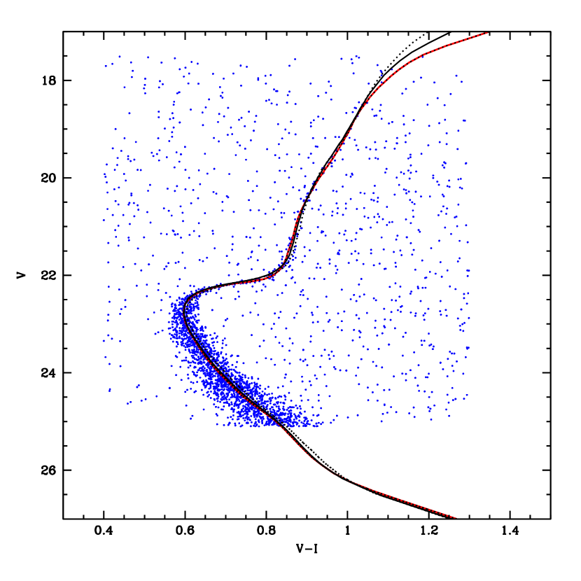
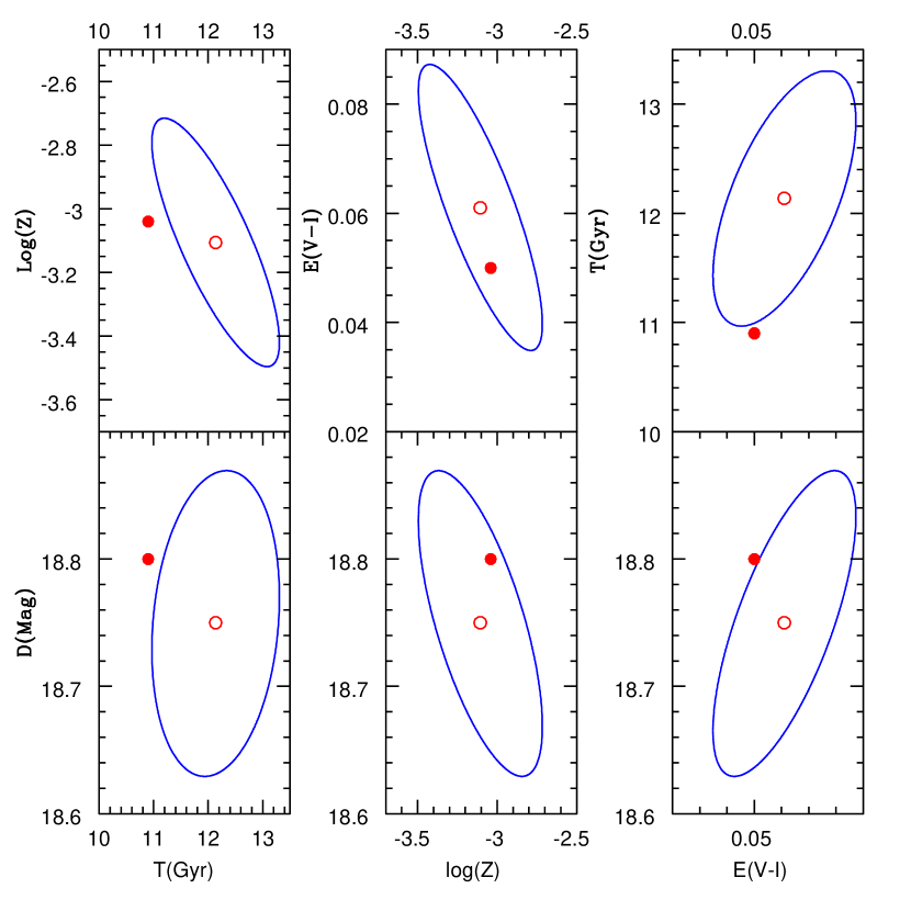
Figure 11: (Left) Simulated Single Stellar Population CMD having an age of 10.9 Gyr and $\log Z=-3.05$. The thick (black) curve shows the input isochrone, with the optimal fit isochrone recovered by the method, appearing as a thin (red) curve. Dotted curves show the youngest and oldest isochrones allowed by the method, at the $1\sigma$ level, which in fact span a 1.78 Gyr interval. (Right) The six panels show the projection of the error ellipsoid resulting from the Monte Carlo simulation and inversion of a SSP with age 10.9 Gyr and metallicity $\log Z=-3.05$, onto different planes, for CMDs including the addition of 60% Galactic pollution stars. The filled circles show the input parameters, and the empty ones the average values for the recovered parameters.

In general, the choice in the details of any implementation will depend on the robustness of the available data and theoretical models. One would expect that with time, stellar modeling will improve to the point of making more reliable predictions, not only for very young stellar populations, but also for stellar phases beyond the helium flash, perhaps even into the white dwarf cooling sequence, and including all the currently poorly understood features like blue stragglers and horizontal branch. At that point, the implementation can be trivially updated by simply changing the range of masses considered along the theoretical isochrone, yielding more accurate and restrictive inferences. On the observational side, when for example GAIA data are available, the effectiveness of the implementation can be improved by including stars further down along the main sequence, to result in improved metallicity and reddening corrections.

The actual stars for this cluster appear in the left panel of Figure 12, together with the best fit isochrone found by the method, using the Yale isochrones, changing the isochrone set, yields results only marginally different. This is clearly seen to be a good fit, obtained this time through a completely automatic and objective procedure, maximizing use of information both from the data and from the stellar models with which the data was compared.

The basic parameters associated to this best fitting isochrone, together with their 1-$\sigma$ confidence intervals are: $T=12.1\pm 0.5$ Gyr, $\log Z=-3.14\pm 0.15$, $D=14.03\pm 0.1$ mag, and E(V-I)$=0.34\pm 0.02$ mag, and are shown in the right panel of Figure 12. As in the previous examples, the method returns not only best fit values and associated statistically robust confidence intervals, but also the full covariance structure of the inference, as shown in Figure 12. We see the 1-$\sigma$ confidence ellipse in the $(T,Z)$ plane slanting as expected from the ’age-metallicity degeneracy’, but again, almost no correlation in the $(T,D)$ plane. Again, when moving along the correlations in the recovered parameters, we see that the maximum and minimum age isochrones, at the 1-$\sigma$ level, dotted curves, are practically indistinguishable from each other, or from the the best fit one, based only on shape. The three solid dots in Figure 12 give the center of our inferences, for three different values of the [$\alpha$/Fe] enhancement parameter, 0.0, +0.3 and +0.6, a final systematic, which also has little effect. The isochrones shown are only for the alpha enhancement of 0.0, as the inclusion of the corresponding isochrones for the other two values would only result in a complete overlapping of curves, all within the region defined by the oldest and youngest isochrones at [$\alpha$/Fe] =0.0 shown. The resolution of the method, as mentioned earlier, is much enhanced from a simple geometric fitting of isochrones by having included the duration of evolutionary phases explicitly in the merit function being used. Confidence intervals similar to the case of Figure 11 are the result of the large number of stars available above the lower magnitude cut.

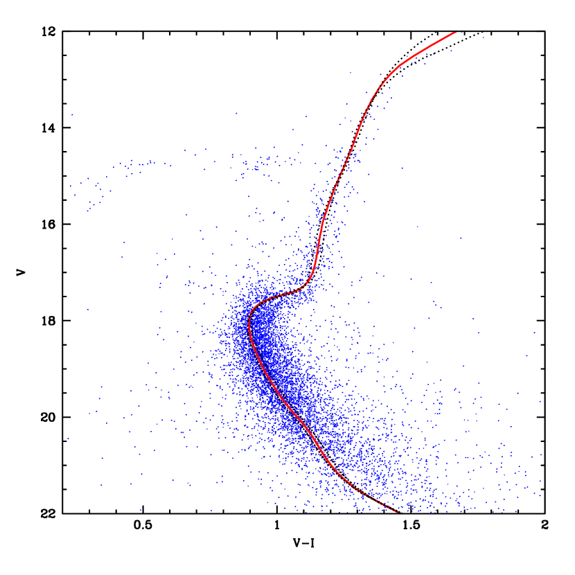
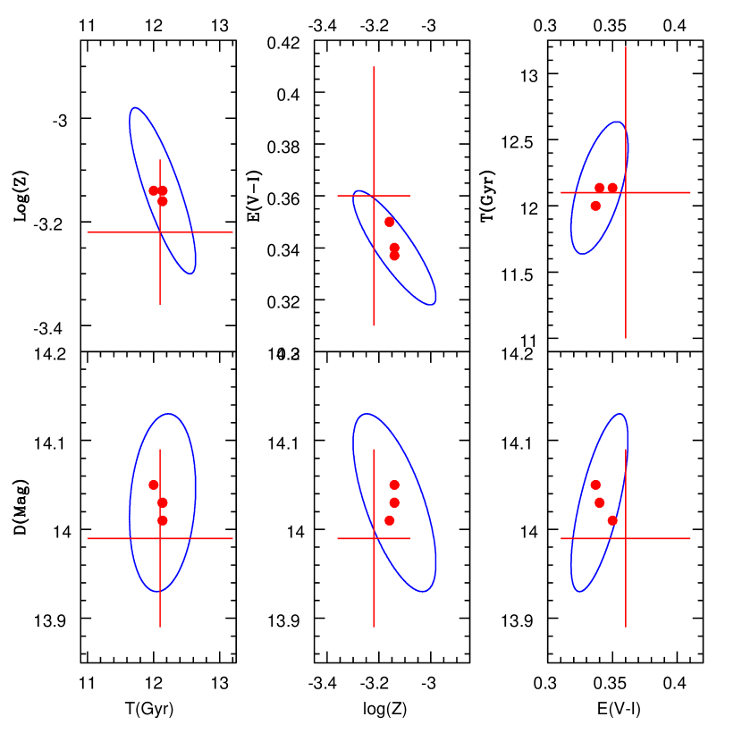
Figure 12: (Left) Observed CMD for NGC 3201. The thick (red) curve shows the optimal fit isochrone recovered by the method. Dotted curves show the youngest and oldest isochrones allowed by the method, at the $1\sigma$ level, which in fact span a $1.0$ Gyr interval. (Right) The six panels show the projection of the error ellipsoid resulting from the Monte Carlo simulation and inversion of a SSP with age 12.1 Gyr and metalicity $\log Z=-3.14$, onto different planes, for CMDs including a similar number of stars, and errors modeled as the reported ones for NGC 3201. Filled circles show the average values for the recovered parameters, for 3 different values of assumed [$\alpha$/Fe] enhancement, 0.0, +0.3 and +0.6, and the crosses give inferences and uncertainties as found in the recent literature for this cluster, see text.

For comparison, in the globular cluster compilation by Harris (1996), NGC 3201 is listed as having $(m-M)_{V}=14.24$ mag, E(B-V) = $0.24$ mag (which translates into E(V-I)=0.25), and a metallicity of $\log Z=-3.28$, with no confidence intervals for any of the above. The more recent Salaris & Weiss (2002) report an age for this cluster of $12.1\pm 1.1$ Gyr, Kraft & Ivans (2003) quote a metalicity of between $\log Z=-3.08$ and $-3.36$, taking the extremes of all the possibilities they give, for different red giant spectral metalicity determinations and a solar value of $\log Z_{\odot}=-1.7$. Rosenberg et al. (2000) give a value for the apparent $D=(m-M)_{V}=14.17$ mag, with no estimates of the associated confidence intervals. Recent determinations of the reddening towards this field include Salaris & Cassisi (1998) giving E(B-V) = $0.24\pm 0.02$ mag (which translates into E(V-I)=0.29 $\pm 0.024$), and Piersimoni et al. (2002) giving E(V-I)=$0.36\pm 0.05$ mag, which compares very well with our measure of E(V-I)=R=$0.34\pm 0.02$. This results in a distance modulus of $\mu=D-1.92$E(V-I) = 13.38$\pm$0.1, which agrees with the determination of Piersimoni et al. (2002) of $\mu=13.31\pm 0.06$ mag based on RR Lyr stars in the cluster.

The crosses in Figure 12 summarize the independent determination for the parameters of NGC 3201 which we treated, as discussed in the text above. Overall, comparing our results for NGC 3201 with independent determinations from the literature, we find very good agreement within the uncertainties of the different determinations, and we notice that our results have typically more restrictive confidence intervals. We see that in spite of the absence of evolutionary phases beyond the helium flash in the models we used, the fit is robust and yields good results. The presence of a level of contamination and a horizontal branch, lead to larger error ellipses than in the controlled experiments of previous sections, but no evidently wrong systematics are apparent, we conclude no large systematics remain. The lower region of the CMD appears more poorly fitted, a consequence of having only considered stars brighter than $V=20$ in the fitting procedure. These lower regions of the CMD however, are heavily affected by incompleteness and very large observational errors, requiring, in the context of the method used, their exclusion.

This results can be seen as an overall validation of the method, as metalicities, distances and reddening corrections reported by the authors cited where often derived through methods completely independent to the stellar evolution model comparisons we have performed here. We find that in going to real data, the expectations of the previous sections hold, and we are able to obtain a best fit solution which is clearly a good solution, the resulting isochrone is a good match to the observed stars, and the values for the $(T,Z,D,R)$ vector obtained match well with completely independent determinations found in the literature. The fit is of course not perfect, and inconsistencies between stellar models and reality undoubtedly remain, even below the turn off region, where available stellar models largely agree with each other. However, the full agreement between our inferences and those derived through completely independent physical and astronomical methods noted above, show that no systematics are being introduced by the remaining inadequacies of stellar evolutionary codes, at least not beyond the confidence intervals internally calculated by the method.

The comparison of results obtained with our method against accurate independent determinations of metalicities through spectroscopy, or distances through future parallax measurements, could hence be used to check stellar evolution theory.

6 Conclusions

We have presented a method which treats the inference of structural parameters of single stellar populations in a fully rigorous statistical manner, within a Bayesian approach, to construct a merit function for the comparison of an observed CMD in relation to a point in the 4-D parameter space of age, metallicity, distance modulus and reddening.

Implementing a genetic algorithm simulation we have shown through various examples using synthetic CMDs with parameters as appropriate for current observations of Galactic Single Stellar Populations, that the method accurately recovers the input parameters, and yields reliable confidence intervals, including naturally an analysis of the covariances and correlations between the recovered parameters.

By performing extensive Monte Carlo experiments with systematic effects, which surely apply to real cases and which are explicitly excluded from the formalism presented, we have evaluated the consequences these effects are expected to have on the results of our method. We found that although the error ranges on the recovered parameters typically increase, no systematic offsets appear, at least within the reasonable ranges tested.

This implies that our formalism, which explicitly takes into account the number density of stars along isochrones, can tentatively test stellar evolution models when using clusters with well-measured abundances, distances and reddenings. This, along with the absolute dating of clusters with precise photometry, will be presented in the second paper of this series (Valls–Gabaud & Hernandez 2007).

References

- (1) Bergbusch, P.A. & VandenBerg, D.A. 1997, AJ, 114, 2604
- (2) Buonanno, R., Corsi, C. E., Pulone, L., Fusi Pecci, F., Bellazzini, M., 1998, A&A, 333, 505
- (3) Cerviño, M., Valls-Gabaud, D., Luridiana, V., Mas-Hesse, J.M., 2002, A&A, 381, 51
- (4) Cerviño, M. & Valls-Gabaud, D., 2003, MNRAS, 338, 481
- (5) Charbonneau, P., 1995, ApJS, 101, 309
- (6) Demarque, P., Woo, J.H., Kim, Y.C., Yi, S.K., 2004, ApJS, 155, 667
- (7) Ferraro, F. R., Messineo, M., Fusi Pecci, F., et al., 1999, AJ, 118, 1738
- (8) Flannery, B.P. & Johnson, B.C. 1982, ApJ, 263, 166
- (9) Girardi, L., et al., 2002, A&A 391, 195
- (10) Georgiev, L. & Hernandez X., 2005, Rev. Mex. A&A, 41, 121
- (11) Harris, W. E., 1996, AJ, 112, 1487
- Hernandez, Valls-Gabaud and Gilmore (1999) Hernandez, X., Valls-Gabaud, D., Gilmore, G., 1999, MNRAS, 304, 705
- Hernandez, Gilmore and Valls-Gabaud (2000a) Hernandez, X., Gilmore, G., Valls-Gabaud, D., 2000a, MNRAS, 317, 831
- Hernandez, Valls-Gabaud and Gilmore (2000b) Hernandez, X., Valls-Gabaud, D., Gilmore, G., 2000b, MNRAS, 316, 605
- (15) Jimenez, R., Padoan, P., 1998, ApJ, 498, 704
- (16) Jørgensen, B., Lindegren, L., 2005, A&A, 436, 127
- (17) Kraft, R. P., Ivans, I., 2003, PASP, 115, 143
- (18) Kroupa, P., Tout, C. A., Gilmore, G., 1993, MNRAS, 262, 545
- (19) Lastennet, E., Valls-Gabaud, D., 2002, A&A, 396, 551
- (20) Metcalfe, T.S., 2003, ApJ, 587, L43
- (21) Naylor, T., Jeffries, R.D., 2006, MNRAS, 373, 1251
- (22) Paczyńsky, B., 1984, ApJ, 284, 670
- (23) Pagel, B.E.J., 1996, ASP Conf. Series 99, 307
- (24) Piersimoni, A. M., Bono, G., Ripepi, V., 2002, AJ, 124, 1528
- (25) Popper, D.M. 1980, ARAA, 18, 115
- (26) Ratcliff, S.J. 1987, ApJ, 318, 196
- (27) Renzini, A., Buzzoni, A., 1983, Mem. Soc. Ast. Ital., 54, 739
- (28) Renzini, A., Fusi Pecci, F., 1988, ARA&A, 26, 199
- (29) Ribas, I. 2006, in Astrophysics of Variable Stars, Sterken, C. and Aerts, C. (eds), ASP Conference Series, Vol. 349, 55
- (30) Robin, A.C. et al. 2003, A&A, 409, 523
- (31) Rosenberg, A., Saviane, I., Piotto, G., Aparicio, A., 1999, AJ, 118, 2306
- (32) Rosenberg, A., I, Piotto, A., Saviane, G., Aparicio, A., 2000, A&A Supp;. Ser., 144, 5
- (33) Salaris, M., Cassisi, S., 1998, MNRAS, 298, 166
- (34) Salaris, M. & Cassisi, S. 2006, Evolution of stars and stellar populations (Chichester: John Wiley & Sons)
- (35) Salaris, M. & Weiss, A. 1998, A&A, 335, 943
- (36) Salaris, M. & Weiss, A. 2002, A&A, 388, 492
- (37) Sevenster, M., Saha, P., Valls-Gabaud, D., Fux, R. 1999, MNRAS, 307, 584
- (38) Straniero, O., Chieffi, A., 1991, ApJS, 76, 525
- (39) Teriaca, L., Banerjee, D., Doyle, J.G. 1999, A&A, 349, 636
- (40) Valls-Gabaud, D. & Hernandez, X. 2007, in preparation (Paper II)
- (41) VandenBerg, D.A., 2000, ApJS, 129, 315
- (42) VandenBerg, D.A., Durrell, P. R., 1990, AJ, 99, 221
- (43) VandenBerg, D.A., Stetson, P.B., Bolte, M., 1996, ARA&A, 34, 461
- (44) VandenBerg, D.A. 2007, in Resolved Stellar Populations, eds. D. Valls-Gabaud & M. Chavez, ASP Conf. Series, in press
- (45) VandenBerg, D.A., Bergbusch, P.A., Dowler, P.D., 2006, ApJS, 162, 375
- (46) Wilson, R.E. & Hurley, J.D. 2003, MNRAS, 344, 1175
- (47) Zoccali, M., Piotto, G., 2000, A&A, 358, 943