Emerging singularities in the bouncing loop cosmology

Abstract

In this paper we calculate $\mathcal{O}(\mu^{4})$ corrections from holonomies in the Loop Quantum Gravity, usually not taken into account. Allowance of the corrections of this kind is equivalent with the choice of the new quatization scheme. Quantization ambiguities in the Loop Quantum Cosmology allow for this additional freedom and presented corrections are consistent with the standard approach. We apply these corrections to the flat FRW cosmological model and calculate the modified Friedmann equation. We show that the bounce appears in the models with the standard $\mathcal{O}(\mu^{2})$ quantization scheme is shifted to the higher energies $\rho_{\text{bounce}}=3\rho_{\text{c}}$. Also a pole in the Hubble parameter appears for $\rho_{\text{pole}}=\frac{3}{2}\rho_{\text{c}}$ corresponding to hyper-inflation/deflation phases. This pole represents a curvature singularity at which the scale factor is finite. In this scenario the singularity and bounce co-exist. Moreover we find that an ordinary bouncing solution appears only when quantum corrections in the lowest order are considered. Higher order corrections can lead to the nonperturbative effects.

I Introduction

Strength of the gauge field $F$ in some point $x$ can be obtained form holonomy calculated around this point and taking limit of the zero length of the loop. Loop Quantum Gravity (LQG) is kind of gauge theory describing gravitational degrees of freedom in terms of gauge field $A$ which is elements of $\mathfrak{su}(2)$ algebra and conjugated variable $E$ which is elements of $\mathfrak{su}(2)^{*}$ algebra Ashtekar:1987gu . To quantise this theory in a background independent way one introduces holonomies of the Ashtekar connection $A$

$$h_{\alpha}[A]=\mathcal{P}\exp\int_{\alpha}A\quad\text{where 1-form}\quad A=\tau_{i}A^{i}_{a}dx^{a}$$ (1)

where $\tau_{i}=-\frac{i}{2}\sigma_{i}$ ($\sigma_{i}$ are Pauli matrices) and conjugated fluxes

$$F_{S}^{i}[E]=\int_{S}dF^{i}\quad\text{where 2-form}\quad dF_{i}=\epsilon_{abc}E^{a}_{i}dx^{b}\wedge dx^{c}$$ (2)

as new fundamental variables Nicolai:2005mc ; Perez:2004hj . Other variables like the field strength $F$ should be expressed in term of these elementary variables. As we mentioned at the beginning the field strength can be expressed in term of holonomies. However, another aspect of loop quantisation starts to be important here. Namely, an area operator possesses a discrete spectrum with minimal nonzero eigenvalue $\Delta$ Ashtekar:1996eg . So we cannot simply shrink to zero the area enclosed by loop. Instead of this we must stop shrinking loop for a minimal value corresponding to the area gap $\Delta$. This effect leads to quantum gravitational corrections to the expression for classical field strength. The expression for the field strength as a function of holonomies have a form Ashtekar:2006wn

$$F^{k}_{ab}=\lim_{\mu\rightarrow\bar{\mu}}\left\{-2\frac{\text{tr}\left[\tau_{k}\left(h^{(\mu)}_{\Box_{ij}}-\mathbb{I}\right)\right]}{\mu^{2}V_{0}^{2/3}}{{}^{o}\omega^{i}_{a}}{{}^{o}\omega^{j}_{b}}+\frac{\mathcal{O}(\mu^{4})}{\mu^{2}}\right\}$$ (3)

where the limit $\mu\rightarrow\bar{\mu}$ corresponds to the minimal value of the area gap $\Delta$. However, this formula is adequate only when $\mathcal{O}(\mu^{4})$ terms can be neglected, i.e., in the classical limit. In fact these terms, which form infinite series, are a function of $F$ and $A$. The expression for the $F$ as a function of holonomies should be therefore obtained by solving this equation in terms of the first factor on the right side. In the classical limit $\mu\rightarrow 0$ terms $\mathcal{O}(\mu^{4})/\mu^{2}$ vanish and we recover a classical expression for the field strength. Until now in literature the first order quantum correction to field strength has been investigated. It means that terms $\mathcal{O}(\mu^{4})$ have been neglected. This approach was dictated be the choice of the simplest quantization scheme. Namely, as it has been shown by Bojowald Bojowald:2006gr ; Bojowald:2007gc ; Bojowald:2008pu , the precise effective Hamiltonian must be a periodic function of the canonical variable $c$. The simplest form of this function we obtain when we perform the regularisation of the expression for the classical field strength cutting off the terms $\mathcal{O}(\mu^{4})$. This is a standard procedure in the Loop Quantum Cosmology.

In this paper we calculate and study another non-vanishing contribution what is in fact a choice of the different regularisation of the expression for the field strength. It means that we hold $\mathcal{O}(\mu^{4})$ factor, which is a function of $F$, and we solve equations for $F$ as a function of the holonomies. This approach is equivalent to the choice of the new quantization scheme what is allowed due to quantization ambiguities.

The organisation of the text is the following. In section II we calculate expression for $F$ as a function of holonomies in $\mathcal{O}(\mu^{4})$ order. Then in section III we apply this result to the flat Friedmann-Robertson-Walker (FRW) cosmological model. We show that obtained correction have important influence for this model. In section V we summarise the results. Finally in the Appendix we give some basics of Loop Quantum Cosmology connected with the subject of this paper and explain the employed notation.

II Holonomy corrections

From the definition (1) we can calculate holonomy for homogeneous model in the particular direction ${}^{o}e^{a}_{i}\partial_{a}$ and the length $\mu V_{0}^{1/3}$

$$h_{i}^{(\mu)}=e^{\tau_{i}\mu c}=\mathbb{I}\cos\left(\frac{\mu c}{2}\right)+2\tau_{i}\sin\left(\frac{\mu c}{2}\right).$$ (4)

From such particular holonomies we can construct a holonomy along the closed curve $\alpha=\Box_{ij}$ as schematically presented in the diagram below

and can be written as

$$h_{\Box_{ij}}^{(\mu)}=h_{i}^{(\mu)}h_{j}^{(\mu)}h_{i}^{(\mu)-1}h_{j}^{(\mu)-1}=e^{\mu B_{i}}e^{\mu B_{j}}e^{-\mu B_{i}}e^{-\mu B_{j}}$$ (5)

where we have introduced

$$B_{i}:=V_{0}^{1/3}A_{a}{{}^{o}e^{a}_{i}}=V_{0}^{1/3}c\tau_{i}.$$ (6)

Factors $B_{i}$ are elements of $\mathfrak{su}(2)$ algebra so to perform product of exponents in equation (5) we need to use the Baker-Campbell-Hausdorff formula

$$e^{X}e^{Y}=\exp\left\{X+Y+\frac{1}{2}[X,Y]+\frac{1}{12}\left([X,[X,Y]]+[Y,[Y,X]]\right)-\frac{1}{24}[Y,[X,[X,Y]]]+\dots\right\}.$$ (7)

To calculate $\mathcal{O}(\mu^{4})$ correction the elements of the expansion written above are sufficient. Applying this formula to equation (5) we obtain

$$h_{\Box_{ij}}^{(\mu)} = \exp\left\{\mu^{2}[B_{i},B_{j}]+\frac{\mu^{3}}{2}[B_{i}+B_{j},[B_{i},B_{j}]]-\frac{\mu^{4}}{12}[B_{j},[B_{i},[B_{i},B_{j}]]]+\frac{\mu^{4}}{6}[B_{i}+B_{j},[B_{i}+B_{j},[B_{i},B_{j}]]]+\mathcal{O}(\mu^{5})\right\}$$ (8)

$$= \mathbb{I}+\mu^{2}[B_{i},B_{j}]+\frac{\mu^{3}}{2}[B_{i}+B_{j},[B_{i},B_{j}]]-\frac{\mu^{4}}{12}[B_{j},[B_{i},[B_{i},B_{j}]]]+\frac{\mu^{4}}{6}[B_{i}+B_{j},[B_{i}+B_{j},[B_{i},B_{j}]]]$$

$$+ \frac{\mu^{4}}{2}[B_{i},B_{j}][B_{i},B_{j}]+\mathcal{O}(\mu^{5}).$$

Now, multiplying this expression by $\tau_{k}$, using definition (6) and taking a trace of both sides we obtain

$$\text{tr}\left[\tau_{k}\left(h^{(\mu)}_{\Box_{ij}}-\mathbb{I}\right)\right] = \mu^{2}c^{2}_{\text{h}}\epsilon_{ijl}\text{tr}\left(\tau_{k}\tau_{l}\right)+\frac{\mu^{3}}{2}c^{3}_{\text{h}}\epsilon_{ijl}(\epsilon_{ilm}+\epsilon_{jlm})\text{tr}\left(\tau_{k}\tau_{m}\right)-\frac{\mu^{4}}{12}c^{4}_{\text{h}}\epsilon_{ijl}\epsilon_{ilm}\epsilon_{jmn}\text{tr}\left(\tau_{k}\tau_{n}\right)$$ (9)

$$+ \frac{\mu^{4}}{6}c^{4}_{\text{h}}\epsilon_{ijl}(\epsilon_{ilm}+\epsilon_{jlm})(\epsilon_{imn}+\epsilon_{jmn})\text{tr}\left(\tau_{k}\tau_{n}\right)+\frac{\mu^{4}}{2}c^{4}_{\text{h}}\epsilon_{ijl}\epsilon_{ijm}\text{tr}\left(\tau_{k}\tau_{l}\tau_{m}\right).$$

We mention that $\{ijk\}$ are external indices and the Einstein summation convention is not fulfilled. The introduced parameter $c_{\text{h}}$ corresponds to the effective canonical variable $c$ which is expressed as a function of holonomies. With use of equation (4) we can directly calculate the left side of equation (9), we obtain

$$\text{tr}\left[\tau_{k}\left(h^{(\mu)}_{\Box_{ij}}-\mathbb{I}\right)\right]=-\frac{\epsilon_{kij}}{2}\sin^{2}\left(\mu c\right).$$ (10)

Then, using properties of $\tau_{i}$ matrices we obtain

$$\frac{1}{3}\mu^{4}c^{4}_{\text{h}}-\mu^{2}c^{2}_{\text{h}}+\sin^{2}\left(\mu c\right)=0.$$ (11)

The $\mathcal{O}(\mu^{3})$ order contribution simply vanishes. The solutions of this equation have a form

$$c^{2}_{\text{h}\pm}=\frac{1\pm\sqrt{1-\frac{4}{3}\sin^{2}\left(\mu c\right)}}{\frac{2}{3}\mu^{2}}.$$ (12)

When we expand the square in the solution for $c^{2}_{\text{h}-}$ we obtain

$$c^{2}_{\text{h}-}=\left[\frac{\sin(\mu c)}{\mu}\right]^{2}+\frac{1}{3}\frac{\sin^{4}(\mu c)}{\mu^{2}}+\dots.$$ (13)

The first factor of the expansion corresponds to the known case when $\mathcal{O}(\mu^{4})$ corrections are ignored. We can easily check than the classical limit $\mu\rightarrow 0,\ c^{2}_{\text{h}}\rightarrow c^{2}$ is recovered only in the $c^{2}_{\text{h}-}$ case. The case $c^{2}_{\text{h}+}$ should be therefore treated as unphysical. However, as we will see in the next section, both solutions lead to the same modified Friedmann equation. So we can keep both solutions.

Finally the expression for the effective field strength has a form

$$F_{ab}^{k}=\epsilon^{k}_{\ ij}\frac{1\pm\sqrt{1-\frac{4}{3}\sin^{2}\left(\bar{\mu}c\right)}}{\frac{2}{3}\bar{\mu}^{2}V_{0}^{2/3}}{{}^{o}\omega^{i}_{a}}{{}^{o}\omega^{j}_{b}}.$$ (14)

We have performed here the limit $\mu\rightarrow\bar{\mu}$ where

$$\bar{\mu}=\sqrt{\frac{\Delta}{|p|}}.$$ (15)

For details of this limit see papers Ashtekar:2006wn or appendices to the papers Chiou:2007mg ; Mielczarek:2008zv ; Magueijo:2007wf .

As we have mentioned earlier the precise effective Hamiltonian must be a periodic function of $c$. In our case the effective Hamiltonian has a form $H_{\text{eff}}\sim\sqrt{|p|}c^{2}_{\text{h}-}$ where the $c^{2}_{\text{h}-}$ can be expressed as

$$c^{2}_{\text{h}-}=\frac{1}{2\bar{\mu}^{2}}\sum_{n=1}^{\infty}\frac{(2n)!}{(2n-1)n!^{2}3^{n-1}(2i)^{2n}}\left[\exp(i\bar{\mu}c)-\exp(-i\bar{\mu}c)\right]^{2n}.$$ (16)

As we see this function is periodic, and forms an infinite series numerated by integers. However, this infinity is allowed in the frames of Loop Quantum Cosmology. The obtained effective Hamiltonian is correct however is not given by the simple function as we should expect for fundamental expressions. However, we should to keep in mind that we are looking for the effective Hamiltonian and there is no circumstances that such a Hamiltonian must have mathematically simple allowed form.

In the next section we will use the calculated effective field strength $F$ for the FRW $k=0$ cosmological model.

III Application to FRW $k=0$

With use of equation (14) we can derive the effective Hamiltonian for the flat FRW model in the form

$$H_{\text{eff}}=-\frac{3}{8\pi G\gamma^{2}}\frac{1\pm\sqrt{1-\frac{4}{3}\sin^{2}\left(\bar{\mu}c\right)}}{\frac{2}{3}\bar{\mu}^{2}}\sqrt{|p|}+{|p|}^{3/2}\rho.$$ (17)

For details we send to the appendix. This Hamiltonian fulfils the so called Hamiltonian constraint $H_{\text{eff}}=0$. From Hamilton equations we can calculate evolution of the canonical variable $p$

$$\dot{p}=\left\{p,H_{\text{eff}}\right\}=-\frac{8\pi G\gamma}{3}\frac{\partial H_{\text{eff}}}{\partial c}$$ (18)

and with use of (17) we obtain

$$\dot{p}=\mp\frac{\sqrt{|p|}}{\gamma\bar{\mu}}\frac{2\sin(\bar{\mu}c)\cos(\bar{\mu}c)}{\sqrt{1-\frac{4}{3}\sin^{2}\left(\bar{\mu}c\right)}}.$$ (19)

Applying equation (19), the Hamiltonian constraint $H_{\text{eff}}=0$ and definition of the Hubble parameter $H=\frac{\dot{p}}{2p}$ we finally derive the modified Friedmann equation

$$H^{2}_{\mathcal{O}(\mu^{4})}=\frac{8\pi G}{3}\rho\left(1-\frac{\rho}{3\rho_{\text{c}}}\right)\left[\frac{3}{4}+\frac{1}{4}\frac{1}{\left(1-\frac{2}{3}\frac{\rho}{\rho_{\text{c}}}\right)^{2}}\right]$$ (20)

where we have introduced

$$\rho_{\text{c}}=\frac{\sqrt{3}}{16\pi^{2}\gamma^{3}l_{\text{Pl}}^{4}}.$$ (21)

As we see obtained equation does not depend on the sign $\pm$ in the Hamiltonian. An analogous equation in the lowest order has been calculated earlier Ashtekar:2006wn and have a form

$$H^{2}_{\mathcal{O}(\mu^{2})}=\frac{8\pi G}{3}\rho\left(1-\frac{\rho}{\rho_{\text{c}}}\right).$$ (22)

This equation lead to the bounce for $\rho=\rho_{\text{c}}$. An analogous bounce is also present in the derived model (20), however now the bounce is shifted to the higher energy densities

$$\rho_{\text{bounce}}=3\rho_{\text{c}}.$$ (23)

Another important property is the pole in the Hubble parameter for

$$\rho_{\text{pole}}=\frac{3}{2}\rho_{\text{c}}$$ (24)

as we see from equation (20). We show these features in Fig. 1. In the left panel we present $H^{2}$ as a function of energy density for $\mathcal{O}(\mu^{2})$ and $\mathcal{O}(\mu^{4})$ cases. In the right panel we compare evolution of the Hubble parameter as a function of $p$ for the radiation dominated Universe $(\rho\propto 1/p^{2})$.

$\begin{array}[]{cc}\includegraphics[width=170.71652pt,angle={270}]{fig1.eps}&\includegraphics[width=170.71652pt,angle={270}]{fig2.eps}\end{array}$

Figure 1: Left : Evolution of $H^{2}_{\mathcal{O}(\mu^{2})}$ (red, bottom curve) and $H^{2}_{\mathcal{O}(\mu^{4})}$ (green, top curve) as a function of energy density $\rho$. The parts below zero value of $H^{2}$ are unphysical. The $\rho$ is in the units of $\rho_{\text{c}}$. Right : Evolution of $H^{2}_{\mathcal{O}(\mu^{2})}$ (red, bottom curve) and $H^{2}_{\mathcal{O}(\mu^{4})}$ (green, top curve) as a function of $p$ for the model with radiation $(\rho\propto 1/p^{2})$. On the both panels a physically admissible region corresponds to $H^{2}\geq 0$.

In both case we observe a nonperturbative feature, namely the pole for $\rho=\frac{3}{2}\rho_{\text{c}}$. This fact indicates that higher order corrections from holonomies can have important influence for dynamical behaviour for small values of $p$. It is clear from a parameter of expansion (15) which grows for small values of $p$. For large $p$ the classical case is clearly recovered, however behaviour for small values of $p$ is highly complicated. Namely, as our study suggests higher order terms of expansion have nonperturbative influence for dynamics and this fact can seriously complicate a simple bouncing universe picture. We investigate this issue in the next section.

IV Qualitative analysis of dynamics

The advantage of qualitative methods of analysis of differential equations Perko is that we obtain all evolutional paths for all admissible initial conditions. In this approach the evolution of the system is represented by trajectories in the phase space and asymptotic states by critical points. We demonstrate that dynamics of the model can be reduced to 2-dimensional autonomous dynamical system. These methods allow to distinguish a generic evolutional scenario.

In Fig. 2 we show the phase portrait for all admissible initial conditions (all values of total energy $E$ of the fictitious particle moving in a $1$-dimensional potential proportional to $p^{3}$) for the model with the free scalar field.

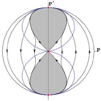
Figure 2: The phase portrait for all admissible initial conditions. The blue line is representing points at which trajectories pass horizontally through the inflection point (hyper-inflationary/deflationary phases).

The physical trajectories are situated in the region at which $E-V$ is non-negative or $p$ is larger than some minimal value and $p^{\prime}$ is zero. The physical trajectories lie in the non-shaded region bounded by a zero velocity curve which represents a homoclinic orbit. Of course the whole system is symmetric with respect to the reflection ($H$ is changed in $-H$). The blue line on the phase portrait represents points at which trajectories pass horizontally through the inflection point (hyper-inflationary/deflationary phases). Therefore, evolution comprises the bounce solution interpolating static phases of evolution, see Fig. 3. There is the intermediate phase of evolution at which we have the inflection point at the diagram of $p(t)$. Note that it is the singularity state with rapid growth of the scale factor, we call this phase the hyper-inflation. It is important to note that energy density is finite during transition through these singularities. Similar finite scale factor singularities has been studied recently by Cannata et al. Cannata:2008xc .

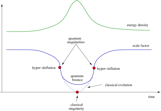
Figure 3: The schematic picture of the evolution of the model. The top curve (green) represents the energy density of the free scalar field. It is worth to note that this energy density is finite during whole evolution, even during transitions through singularities. The bottom curve (blue) presents schematic evolution of the scale factor for the investigated model. The dashed curve represents the classical evolution which is not realised in the presented quantum model.

In the phase diagram in Fig. 2 we adjoint a circle at infinity in standard way via Poincare construction. Note that all trajectories are starting from unstable node - representing static Einstein Universe and landing at stable node representing another static Einstein Universe.

Parisi et al. Parisi:2007kv pointed out that stability of Einstein static models in high-energy modifications of General Relativity is important from the point of view of so-called Emergent Universe scenario Ellis:2002we . Mulryne et al. Mulryne:2005ef investigated the stability of the Einstein static model and they found that LQC Einstein static model is representing a centre type of critical point on the phase portrait. As it is well known such a critical point is structurally unstable. Note that in our case this static universe is representing a node type of critical point. This modification of stability in presented model has important consequences for the Emergent Universe scenario, since as it is well known in General Relativity, a static Universe is unstable and is represented by a saddle type of critical point and therefore it requires the fine-tuning. Moreover corrections considered lead to a regularization of the big-bang singularity Bojowald:2001xe .

V Summary

In this paper we have calculated another non-vanishing contribution to the quantum holonomy correction in Loop Quantum Gravity. Quantum correction of this kind appears when we express the Ashtekar connection $A$ and field strength $F$ in terms of holonomies. The source of quantum modification to classical expressions is a non-vanishing area enclosed by loop as the result of existence of the area gap $\Delta$.

We had applied obtained corrections to the flat FRW cosmological model and the we have calculated resulting quantum gravitational modifications to the Friedmann equation. The holonomy correction in the lowest order to the flat FRW model has been calculated earlier Ashtekar:2006rx ; Ashtekar:2006uz ; Ashtekar:2006wn and extensively studied Singh:2006im ; Mielczarek:2008zv . These investigations uncovered existence of the bounce for energy scales $\rho_{\text{c}}$. In this picture the standard Big Bang singularity is replaced by the non-singular Big Bounce. Calculations performed in the present paper indicate that the holonomy correction in the next non-vanishing order holds this picture. Namely, the initial singularity is still preserved. However the bounce appears now for higher energy density $\rho_{\text{bounce}}=3\rho_{\text{c}}$. Another important new feature is the appearance of a pole in the Hubble parameter for $\rho_{\text{pole}}=\frac{3}{2}\rho_{\text{c}}$ corresponding to hyper-inflationary/deflationary phases. This leads to more complicated dynamical behaviour at these energy scales.

We showed that the generic evolutional scenario for the model with the free scalar field starts from the static Einstein universe then recolapse passing through the curvature singularity with a finite scale factor (hyper-deflation) towards the bounce and goes in the expanding phase through the second curvature singularity (hyper-inflation) and ends in the static Einstein universe. During the transition through the singularities the universal critical behaviour $H\propto|\rho-\rho_{\text{pole}}|^{-1}$ holds. Therefore in the presented scenario the bounce connects these two finite scale factor singularities.

As we see, the higher order quantum correction in LQG can have an important influence on dynamical behaviour of cosmological models. It is not unlikely that the non-singular bounce appeared in the lowest order can be only an artifact of simplifications and can disappear when whole contribution will be taken into account. Further investigations of quantum corrections from LQG are still necessary. We conclude that higher order holonomy corrections and resulting different quantization schemes should be also seriously taken into account in considerations.

Appendix A Flat FRW model in Loop Quantum Gravity

The FRW $k=0$ spacetime metric can be written as

$$ds^{2}=-N^{2}(x)dt^{2}+q_{ab}dx^{a}dx^{b}$$ (25)

where $N(x)$ is the lapse function and the spatial part of the metric is expressed as

$$q_{ab}=\delta_{ij}{\omega^{i}_{a}}{\omega^{j}_{b}}=a^{2}(t){{}^{o}q}_{ab}=a^{2}(t)\delta_{ij}{{}^{o}\omega^{i}_{a}}{{}^{o}\omega^{j}_{b}}.$$ (26)

In this expression ${{}^{o}q}_{ab}$ is fiducial metric and ${{}^{o}\omega^{i}_{a}}$ are co-triads dual to the triads ${{}^{o}e^{a}_{i}}$, ${{}^{o}\omega^{i}}({{}^{o}e_{j}})=\delta^{i}_{j}$ where ${}^{o}\omega^{i}={{}^{o}\omega^{i}_{a}}dx^{a}$ and ${}^{o}e_{i}={{}^{o}e_{i}^{a}}\partial_{a}$. From these triads we construct the Ashtekar variables

$$A^{i}_{a} \equiv \Gamma^{i}_{a}+\gamma K_{a}^{i}=cV_{0}^{-1/3}\ {{}^{o}\omega^{i}_{a}},$$ (27)

$$E^{a}_{i} \equiv \sqrt{|\det q|}e^{a}_{i}=pV_{0}^{-2/3}\sqrt{{}^{o}q}\ {{}^{o}e^{a}_{i}}$$ (28)

where

$$|p| = a^{2}V_{0}^{2/3},$$ (29)

$$c = \gamma\dot{a}V_{0}^{1/3}.$$ (30)

Note that the Gaussian constraint implies that $p\leftrightarrow-p$ leads to the same physical results. The factor $\gamma$ is called the Barbero-Immirzi parameter, $\gamma=\ln 2/(\pi\sqrt{3})$. In the definition (27) the spin connection is defined as

$$\Gamma^{i}_{a}=-\epsilon^{ijk}e^{b}_{j}(\partial_{[a}e^{k}_{b]}+\frac{1}{2}e^{c}_{k}e^{l}_{a}\partial_{[c}e^{l}_{b]})$$ (31)

and the extrinsic curvature is defined as

$$K_{ab}=\frac{1}{2N}\left[\dot{q}_{ab}-2D_{(a}N_{b)}\right]$$ (32)

what corresponds to $K^{i}_{a}:=K_{ab}e^{b}_{i}$.

The scalar constraint, in the Ashtekar variables, has the form

$$H_{\rm G}=\frac{1}{16\pi G}\int_{\Sigma}d^{3}xN(x)\frac{E^{a}_{i}E^{b}_{j}}{\sqrt{|\mathrm{det}E|}}\left[{\varepsilon^{ij}}_{k}F_{ab}^{k}-2(1+\gamma^{2})K^{i}_{[a}K^{j}_{b]}\right]$$ (33)

where field strength is expressed as

$$F^{k}_{ab}=\partial_{a}A^{k}_{b}-\partial_{b}A^{k}_{a}+\epsilon^{k}_{\ ij}A^{i}_{a}A^{j}_{b}.$$ (34)

With use of (27),(28) and (34) the Hamiltonian (33) assumes the form

$$H_{\text{G}}=-\frac{3}{8\pi G\gamma^{2}}\sqrt{|p|}c^{2}$$ (35)

where we have assumed a gauge of $N(x)=1$. Quantum corrections to this Hamiltonian come when we express $\sqrt{|p|}$ and $c^{2}$ in terms of background independent variables. In this paper we had concentrated on the corrections to the factor $c^{2}$, called holonomy corrections. For a short review of quantum corrections we send to the appendix in the paper Magueijo:2007wf .

References

- (1) A. Ashtekar, Phys. Rev. D 36 (1987) 1587.
- (2) H. Nicolai, K. Peeters and M. Zamaklar, Class. Quant. Grav. 22 (2005) R193 [arXiv:hep-th/0501114].
- (3) A. Perez, arXiv:gr-qc/0409061.
- (4) A. Ashtekar and J. Lewandowski, Class. Quant. Grav. 14 (1997) A55 [arXiv:gr-qc/9602046].
- (5) A. Ashtekar, T. Pawlowski and P. Singh, Phys. Rev. D 74 (2006) 084003 [arXiv:gr-qc/0607039].
- (6) M. Bojowald, Phys. Rev. D 74 (2007) 081301 [arXiv:gr-qc/0608100].
- (7) M. Bojowald, arXiv:0710.4919 [gr-qc].
- (8) M. Bojowald, arXiv:0801.4001 [gr-qc].
- (9) D. W. Chiou, Phys. Rev. D 76 (2007) 124037 [arXiv:0710.0416 [gr-qc]].
- (10) J. Mielczarek, T. Stachowiak and M. Szydlowski, arXiv:0801.0502 [gr-qc].
- (11) J. Magueijo and P. Singh, Phys. Rev. D 76 (2007) 023510 [arXiv:astro-ph/0703566].
- (12) L. Perko, “Differential Equations and Dynamical Systems “, Springer-Verlag, New York 1991.
- (13) F. Cannata, A. Y. Kamenshchik and D. Regoli, arXiv:0801.2348 [gr-qc].
- (14) L. Parisi, M. Bruni, R. Maartens and K. Vandersloot, Class. Quant. Grav. 24 (2007) 6243 [arXiv:0706.4431 [gr-qc]].
- (15) G. F. R. Ellis and R. Maartens, Class. Quant. Grav. 21 (2004) 223 [arXiv:gr-qc/0211082].
- (16) D. J. Mulryne, R. Tavakol, J. E. Lidsey and G. F. R. Ellis, Phys. Rev. D 71 (2005) 123512 [arXiv:astro-ph/0502589].
- (17) M. Bojowald, Phys. Rev. Lett. 86 (2001) 5227 [arXiv:gr-qc/0102069].
- (18) A. Ashtekar, T. Pawlowski and P. Singh, Phys. Rev. Lett. 96 (2006) 141301 [arXiv:gr-qc/0602086].
- (19) A. Ashtekar, T. Pawlowski and P. Singh, Phys. Rev. D 73 (2006) 124038 [arXiv:gr-qc/0604013].
- (20) P. Singh, K. Vandersloot and G. V. Vereshchagin, Phys. Rev. D 74 (2006) 043510 [arXiv:gr-qc/0606032].