ULB-TH/07-35

Gauge Theory RG Flows
from
a Warped Resolved Orbifold

Chethan KRISHNAN and Stanislav KUPERSTEIN

International Solvay Institutes,
Physique Théorique et Mathématique,
ULB C.P. 231, Université Libre de Bruxelles,
B-1050, Bruxelles, Belgium

Abstract

We study gauge-string duality of D3-branes localized at a point on the resolution of the ALE orbifold ${\mathbb{C}}^{3}/{\mathbb{Z}}_{3}$. By explicitly solving for the warp factor, we demonstrate the holographic RG flow from $AdS_{5}\times S^{5}/{\mathbb{Z}}_{3}$ (far away from the resolution) to the usual $AdS_{5}\times S^{5}$ (close to the stack). On the gauge theory side, this maps to the flow between the quiver gauge theory and ${\cal N}=4$ super Yang-Mills. We present two possible scenarios for this RG flow depending on the choice of the VEVs. In particular, one of the scenarios proceeds by two steps involving both Higgsing and confinement.

1 Introduction

One powerful way of constructing gauge theories with reduced supersymmetry in string theory is to consider stacks of D-branes at Calabi-Yau singularities [1]. The original proposal of the AdS/CFT correspondence [2] compared string theory on the near-horizon region of a stack of D3-branes in flat space to the low energy ${\cal N}=4$ super Yang-Mills theory living on the branes. The zoom-in involved in the near-horizon limit washes out all the details of the original background, so changing the background geometry from flat to curved does not result in new gauge theories. One way to get past this problem and to construct new gauge theories, is to look at D3-branes not at a smooth point, but instead at the tip of a Calabi-Yau cone. If the cone $Y_{6}$ is a 6-dimensional real cone over a compact base space $X_{5}$, then the near-horizon limit gives rise to string theory on $AdS_{5}\times X_{5}$ and the dual gauge theory is generically a quiver theory whose details depend on the nature of the singularity.

To construct phenomenologically interesting theories, we need less supersymmetry and we also need to break conformal invariance. One way to break some of the SUSY is to replace the $S^{5}$ in $AdS_{5}\times S^{5}$ with an orbifold $S^{5}/\Gamma$, where $\Gamma$ is a discrete group. This amounts to considering ${\mathbb{R}}^{3,1}\times{\mathbb{R}}^{6}/\Gamma$ instead of ${\mathbb{R}}^{9,1}={\mathbb{R}}^{3,1}\times{\mathbb{R}}^{6}$ before the near-horizon limit. If $\Gamma\in SU(2)$, then the dual theory is ${\cal N}=2$, and if $\Gamma\notin SU(2)$ then we have an ${\cal N}=1$ gauge theory. In this paper, we will consider the case $\Gamma={\mathbb{Z}}_{3}$ and the dual ${\cal N}=1$ superconformal quiver. Another class of examples with reduced supersymmetry where the explicit Ricci-flat metric on the cone is known, is when the base $X_{5}$ is topologically $S^{2}\times S^{3}$. The most extensively investigated gauge-theory/singular-geometry dual of this kind is where $Y_{6}$ is chosen to be the conifold [9], so that the base space is a coset space called $T^{1,1}$. More general classes of Ricci-flat metrics on cones over $S^{2}\times S^{3}$ are also known, leading to the so-called $Y^{p,q}$ and (even more general) $L^{a,b,c}$ spaces and their ${\cal N}=1$ gauge theory duals [16, 40, 41, 42, 43, 44, 45, 46, 47, 48, 49, 50, 51, 52, 21, 53, 54, 55, 29, 30].

In [1, 3], the dual ${\cal N}=1$ superconformal gauge theory corresponding to a stack of $N$ D3-branes at the tip of the conifold was argued to be an $SU(N)\times SU(N)$ gauge theory with matter content given by two chiral superfields $A_{i}$ and $B_{i}$ (where $i=1,2$). The fields $A_{i}$ transform in $(N,\bar{N})$ of $SU(N)\times SU(N)$ while $B_{i}$ transform in $(\bar{N},N)$. The gauge theory on the singular conifold corresponds to the case where none of the fields have a VEV, and the theory is conformal.

To break conformal invariance, we need to look at a space that is not a cone, because the radial direction of the cone is what gets absorbed into the $AdS^{5}$ when we take the near-horizon limit. In the case of the conifold theory described above, there are two ways in which we can accomplish this. One is to deform it by considering a non-vanishing $S^{3}$ at the tip, and the other is to resolve it and keep the $S^{2}$. The former case was the subject of the celebrated paper of Klebanov and Strassler [32] where the deformed $S^{3}$ is supported by a non-vanishing $3$-form flux. The dual theory was found to be a cascading gauge theory (related, but different, from the gauge theory on the singular space). The resolved conifold has also been investigated, but in the dual gauge theory, it corresponds to giving a non-zero VEV for the operator

$$\mathcal{U}=\frac{1}{N}{\rm Tr}\left(\left|A_{1}^{2}\right|+\left|A_{2}^{2}\right|-\left|B_{1}^{2}\right|-\left|B_{2}^{2}\right|\right)$$ (1.1)

in the same $SU(N)\times SU(N)$ gauge theory encountered in the case of the singular conifold. The dual supergravity solution under the assumption that the branes are smeared on the $S^{2}$ was constructed in [13]. The solution they found was singular, as expected. Ideally though, one would like to see the RG flow created by the specific non-zero VEVs on the supergravity side as well, and see the flow from $AdS_{5}\times T^{1,1}$ in the UV to $AdS^{5}\times S^{5}$ near the stack, when the stack is localized on a specific point on the resolution. This was accomplished in [12], where they found the precise form of the warp factor.

In this paper we consider instead the space ${\mathbb{C}}^{3}/{\mathbb{Z}}^{3}$, which after the near-horizon limit gives rise to $AdS_{5}\times S^{5}/{\mathbb{Z}}_{3}$. We look at the case where the space gets a resolution, and the orbifold singularity is replaced by a four-cycle instead of the two-cycle of the conifold. This four-cycle is the projective space ${\mathbb{C}}{\mathbb{P}}^{2}$. We consider the case where the stack of D-branes is localized on a point on the resolution. Far away from the resolution, we see that the warp factor tends to the unresolved case while close to the stack we see the emergence of the $AdS$ throat because the stack is no longer at a singular point. Exactly like in the conifold case there is a single parameter in the resolved metric, which controls the size of the “blown-up” cycle. In the dual gauge theory, this results in a non-zero VEV for a six-dimensional, yet to be constructed [39] operator. On the gauge theory side it corresponds to the fact that all baryonic symmetries are anomalous and no simple current of the form (1.1) is preserved. It means, that unlike in the conifold case there is no straight-forward way to figure out what fields acquire VEVs. However, using the relation between the holomorphic coordinates on the orbifold and the chiral superfields of the gauge theory we found that there are only two non-identical patterns for the RG flow triggered by different VEVs of the fields. In both cases the VEVs breaks the conformal invariance and launches an RG flow that yields the ${\cal N}=4$ SYM, but one of the two scenarios is more complicated then the other and involves two steps involving Higgsing and confinement, the details of which are presented in Section 5.

The structure of this paper is as follows. In the next section we explain the geometry of the orbifold and its resolution. In Section 3 we explain the supergravity solution corresponding to D3-branes on the unresolved space, and the corresponding dual quiver gauge theory. The next two sections are dedicated to the construction of the solution in the resolved space and a discussion of the RG flow on both the gravity and gauge theory sides of the duality. We end in the final section with some discussions and comments. Some of the technical details can be found in the appendices.

Various other aspects of the ${\mathbb{C}}^{3}/{\mathbb{Z}}_{3}$ orbifold have been studied in [10, 15, 7, 33]. Other recent papers which are of relevance to our work are [34, 35, 36, 37, 38].

2 The Toric Description of ${\mathbb{C}}^{3}/{\mathbb{Z}}_{3}$ and its Resolution

The space ${\mathbb{C}}^{3}/{\mathbb{Z}}_{3}$ is defined as the three-dimensional complex space ${\mathbb{C}}^{3}$ under the identification

$$\{w_{1},w_{2},w_{3}\}=\{\eta w_{1},\eta w_{2},\eta w_{3}\},\ {\rm with}\ \eta^{3}=1.$$ (2.1)

Clearly, the only orbifold point is the origin. The orbifold inherits the metric

$$ds_{6}^{2}=dr^{2}+r^{2}d\Omega_{S^{5}/{\mathbb{Z}}_{3}}^{2}$$ (2.2)

from the flat metric on ${\mathbb{C}}^{3}$. The subscript on the angular part is supposed to indicate that the periodicities of the angles are of the orbifold, not of flat space.

There is another, more algebraic, way in which we could define the above orbifold. This turns out to be very useful for comparisons with the gauge theory, so we explain it now. The idea is that the orbifold is fully defined by the invariant (under the orbifold action) monomials that one can construct from the coordinates $w_{i}$. There are ten such monomials as is easily checked, and the domain over which these collection of monomials is well-defined is precisely ${\mathbb{C}}^{3}/{\mathbb{Z}}_{3}$. So one could also define our orbifold by

$${\mathbb{C}}^{3}/{\mathbb{Z}}_{3}={\mathbb{C}}[w_{1}^{3},\,w_{1}^{2}w_{2},\,w_{1}^{2}w_{3},\,w_{2}^{3},\,w_{2}^{2}w_{1},w_{2}^{2}w_{3},\,w_{3}^{3},\,w_{3}^{2}w_{1},\,w_{3}^{2}w_{2},\,w_{1}w_{2}w_{3}].$$ (2.3)

If we call these monomials $U_{ijk}$, with indices ${i,j,k}={1,2,3}$, then the algebraic relations between $U_{ijk}$ (e.g., $U_{112}U_{123}=U_{223}U_{111}$) captures the geometry of the orbifold. It should be understood that $U_{ijk}$ with different permutations of $i,j,k$ are identified. So we could also write,

$${\mathbb{C}}^{3}/{\mathbb{Z}}_{3}={\mathbb{C}}[U_{ijk}]/\{{\rm algebraic\ relations\ between\ the}\ U_{ijk}{\rm{}^{\prime}s}\}.$$ (2.4)

Another important useful fact about ${\mathbb{C}}_{3}/{\mathbb{Z}}_{3}$ is that it is toric. A quick and practical introduction to toric geometry can be found in appendix B of [29] or section 4 of [4]. Essentially, in the present context toric means that all the information about the space (as a complex variety) can be captured using a cone that has its apex at the origin of a 3-dimensional integer lattice. There are qualifications that need to be added to the cone to make this more precise, but instead of stating them, we will refer the exacting reader to [4, 5, 6]. In any event, it turns out that the cone that defines our orbifold can be specified by the (rational) vertices that span it:

$$v_{1}=(-1,0,1),\ \ v_{2}=(0,-1,1),\ \ v_{3}=(1,1,1).$$ (2.5)

One feature of toric spaces that are in addition Calabi-Yau is that their vertices (other that the origin) all have to lie on the same plane. Thus, we can capture them on the toric diagram presented in Fig. 1.

Figure 1: Toric Diagram of ${\mathbb{C}}^{3}/{\mathbb{Z}}_{3}$.

Toric diagrams are useful because many questions about the original space can be answered in terms of simple geometrical features of the diagram. The Calabi-Yau property being translated into co-planarity of vertices is a simple example. Another question that is readily answered is the question of singularities and their resolutions. In fact, the way in which the fact that ${\mathbb{C}}^{3}/{\mathbb{Z}}_{3}$ is singular is captured by our toric diagram is through the presence of a vertex, marked 4 in figure 1, in its interior. In general, if the volume of the cone with origin as its apex is greater than one, then the space is singular. Notice that the volume can be greater than one only if there is an interior point (which in our case is the vertex marked 4). This motivates the following simple recipe for resolving our singular space: add more vertices in the interior in such a way that the new cones have no vertices in their interior, and then look at the resulting collection of cones (the “fan”) as the new space. In our case, since there is only one interior point, ${\mathbb{C}}^{3}/{\mathbb{Z}}_{3}$ has a unique (“crepant”) resolution, and the fan for the resolved space will involve the three new cones that have been created by the addition of vertex 4.

We will be interested in the resolution of the orbifold in later sections, so we make some comments about that here. The vector for vertex 4 is easily seen to be

$$v_{4}=(0,0,1).$$ (2.6)

Clearly, the four vertices should satisfy 4 (= no. of vertices) - 3 (= dimensionality of the lattice) = 1 linear relation between them, which we write as

$$\sum_{i=1}^{4}Q_{i}v_{i}=0,\ {\rm with}\ Q_{i}=(1,1,1,-3).$$ (2.7)

The reason why these charges $Q_{i}$ are interesting is because the translation between the toric diagram and the actual space we are interested in, is effected through them. This is done by means of the “quotient construction” as follows. Pick 4 (= no. of vertices) complex coordinates $z_{i}$. We can define a ${\mathbb{C}}^{*}$-action on these coordinates

$$(z_{1},z_{2},z_{3},z_{4})\rightarrow(\lambda z_{1},\lambda z_{2},\lambda z_{3},\lambda^{-3}z_{4}),\ \lambda\in{\mathbb{C}}^{*},$$ (2.8)

where the powers are the charges above. At this stage, we are only defining the action, we have not yet modded out by anything. The space now is constructed by first imposing

$$|z_{1}|^{2}+|z_{2}|^{2}+|z_{3}|^{2}-3|z_{4}|^{2}=\mu,$$ (2.9)

and then modding out by the phase part (the $U(1)$’s) of (2.8). This should be compared to the two-step construction of ${\mathbb{C}}{\mathbb{P}}^{1}$ by first setting $|z_{1}|^{2}+|z_{2}|^{2}=\mu$ in ${\mathbb{C}}^{2}$, and then modding out by phases, instead of modding out by ${\mathbb{C}}^{*}$ in one go. Notice that the charges $Q$ affect both steps of the quotienting operation (2.9)-(2.8). This quotient construction of the geometry finds its gauge theory analogue in the description of the moduli space in terms of D-terms and is the basis for Witten’s Gauged Linear Sigma Model (GLSM) construction [8] applied to ${\cal N}=1$ theories.

Now, we can try to see how this toric construction of (the resolution of) ${\mathbb{C}}^{3}/{\mathbb{Z}}_{3}$ ties up with the earlier definitions. First we notice that instead of doing the $U(1)$ quotienting, we can parametrise the space through the zero-charge monomials defined by

$$z_{1}^{3}z_{4},\,z_{1}^{2}z_{2}z_{4},\,z_{1}^{2}z_{3}z_{4},\,z_{2}^{3}z_{4},\,z_{2}^{2}z_{1}z_{4},z_{2}^{2}z_{3}z_{4},\,z_{3}^{3}z_{4},\,z_{3}^{2}z_{1}z_{4},\,z_{3}^{2}z_{2}z_{4},\,z_{1}z_{2}z_{3}z_{4}.$$ (2.10)

Obviously, these monomials satisfy the same algebra as the $U_{ijk}$’s in (2.3).

We claim that $\mu=0$ corresponds to the unresolved case, and when $\mu>0$ we get the resolved space where the origin is replaced by a ${\mathbb{C}}{\mathbb{P}}^{2}$. For this, first note that when $z_{4}=0$, all the monomials above are zero, which corresponds to the orbifold point in the language of the $U_{ijk}$’s. But from (2.9) it is clear that when $\mu=0$, $z_{4}=0$ forces $z_{1,2,3}$ to be zero and therefore we end up with a single point, but when $\mu>0$, setting $z_{4}=0$ results in a ${\mathbb{C}}{\mathbb{P}}^{2}$. Thus, $\mu$ can be thought of as the size of the ${\mathbb{C}}{\mathbb{P}}^{2}$ on the resolved orbifold, and when it is zero we end up with ${\mathbb{C}}^{3}/{\mathbb{Z}}_{3}$. It is also possible to see the resolution using only the monomials $U_{ijk}$ similar to the famous conifold construction of [9]. It follows from the algebra satisfied by $U_{ijk}$’s that all $3$d complex vectors of the form

$$v_{jk}^{T}\equiv\left(U_{1jk},U_{2jk},U_{3jk}\right)$$ (2.11)

lie on the same $2$d plane, which means that there exists a $3$d vector $\lambda$ we have

$$v_{jk}^{T}\cdot\lambda=0\qquad{\rm for\,\,any}\quad j,k.$$ (2.12)

This fact follows directly from relations of the form $U_{1jk}U_{2j^{\prime}k^{\prime}}=U_{2jk}U_{1j^{\prime}k^{\prime}}$. The existence of $\lambda$ becomes even more evident if we notice that $v_{jk}^{T}=z_{j}z_{k}(z_{1},z_{2},z_{3})$ for arbitrary $j$ and $k$. Now, the non-zero vector $\lambda$ is fixed up to an overall re-scaling, which means that it defines a point on ${\mathbb{C}}{\mathbb{P}}^{2}$. Furthermore, $\lambda$ is well-defined everywhere except the origin, where all the vectors $v_{jk}$ are identically zero. At the apex $\lambda$ is however un-restricted and we resolve the orbifold by replacing the singular point with the $\lambda$-parametrized ${\mathbb{C}}{\mathbb{P}}^{2}$. This is exactly the same ${\mathbb{C}}{\mathbb{P}}^{2}$ we found setting $\mu>0$.

Before we leave the geometry, we add some comments about how Higgsing in the gauge theory is described in the geometry. When $\mu>0$ and $z_{4}=0$ the rest of the coordinates in (2.9) define ${\mathbb{C}}{\mathbb{P}}^{2}$. Let us assume that $\left|z_{3}\right|$ is of the same order of magnitude as the parameter $\mu$. It means that we consider the $z_{3}\neq 0$ patch of the ${\mathbb{C}}{\mathbb{P}}^{2}$. On this patch we can introduce the coordinates $u_{1}\equiv z_{1}/z_{3}$ and $u_{2}\equiv z_{2}/z_{3}$. Together with the monomial $U_{333}=z_{3}^{3}z_{4}$ these coordinates parametrise the entire patch $z_{3}\neq 0$. Indeed, starting from the set $(u_{1},u_{2},U_{333})$ we can easily determine the rest of the $U_{ijk}$’s. For example, we have $U_{123}=u_{1}u_{2}U_{333}$. If we now send $\mu\to\infty$ still focusing on the $z_{3}\neq 0$ patch we arrive at the regular ${\mathbb{C}}^{3}$ parametrized by $u_{1}$, $u_{2}$ and $U_{333}$. On the toric diagram it looks like we “chop” off the 3d node, while in the dual gauge theory it corresponds to the RG flow to the ${\cal N}=4$ SYM theory.

3 Gauge-String Duality on the Unresolved Orbifold

3.1 Supergravity with Brane Sources

When we put a stack of D3-branes in some background, they act as sources for the type IIB supergravity equations of motion. There is a standard ansätz for solving these equations of motion (see e.g. [11]), which is given by the following prescriptions for the various fields (the metric, the dilaton and the five-form):

$$ds^{2}=H^{-1/2}(y)\eta_{\mu\nu}dx^{\mu}dx^{\nu}+H^{1/2}(y)ds_{6}^{2},\hskip 21.68121pt$$ (3.1)

$$\Phi={\rm const}.,\ \ F_{5}=(1+*)dH^{-1}\wedge dx^{0}\wedge...\wedge dx^{3},$$ (3.2)

The $*$ stands for the Hodge dual operator. The $ds_{6}^{2}$ piece in the metric denotes the dimensions transverse to the D3-branes, and is given in our case by (2.2). The worldvolume (3+1)-metric of the D-branes is Minkowskian, and the entire solution is essentially given by one function, $H(y)$, where $y$ denotes the coordinates on the transverse space. This function is called the warp factor. With this ansätz, the supergravity EOMs (with source terms for the branes) reduce to a single equation, the Green’s equation on the transverse space ($y_{0}$ denotes the location of the stack):

$$\Box_{y}H(y,y_{0})=-\frac{C}{\sqrt{g_{6}}}\delta^{6}(y-y_{0}).$$ (3.3)

We denote the determinant of the 6-metric by $g_{6}$. The strength of the source is captured by $C=2\kappa_{10}^{2}T_{3}N=(2\pi)^{4}g_{s}N\alpha^{\prime 2}$ where $T_{3}=1/(8\pi^{3}g_{s}\alpha^{\prime 2})$ is the brane tension and $\kappa_{10}=8\pi^{7/2}g_{s}\alpha^{\prime 2}$ is the 10-D Newton’s constant.

For the case of the unresolved ${\mathbb{C}}^{3}/{\mathbb{Z}}_{3}$, when we place the stack at the orbifold singularity, this equation can be immediately solved because the warp factor depends only on the radial coordinate. Green’s equation takes the form

$$\frac{1}{r^{5}}\frac{\partial}{\partial r}\Big{(}r^{5}\frac{\partial}{\partial r}H\Big{)}=-\frac{3C}{\pi^{3}r^{5}}\delta(r).$$ (3.4)

The normalization of the delta function accounts for the fact that we are ignoring the angular dependence, it comes from an integral over the angles. Away from the origin the equation is easily integrated, and integrating over the delta function fixes the constant of integration:

$$H(r)=\frac{L^{4}}{r^{4}}\ \ {\rm where}\ \ L^{4}=12\pi g_{s}N\alpha^{\prime 2}.$$ (3.5)

With the usual substitution $z=L^{2}/r$, we end up with

$$ds^{2}=\frac{L^{2}}{z^{2}}(dz^{2}+\eta_{\mu\nu}dx^{\mu}dx^{\nu})+L^{2}d\Omega_{S^{5}/{\mathbb{Z}}_{3}}$$ (3.6)

which is nothing but $AdS^{5}\times S^{5}/{\mathbb{Z}}_{3}$ with equal radii ($=L$) for both the AdS and the $S^{5}/{\mathbb{Z}}_{3}$.

Another thing that we could do is to put the stack away from the tip, in which case we expect that far away, the solution should still look like the one we found above. But close to the stack, now we should see the emergence of the AdS throat because the stack is now at a smooth point. The full solution will have a singularity at $r=0$. We verify these expectations explicitly in an appendix.

The general picture is that when the stack is at the singularity we have the $AdS^{5}\times S^{5}/{\mathbb{Z}}_{3}$ background, and this corresponds to zero VEVs for the fields in the dual gauge theory. When we resolve the space, that is equivalent to turning on specific VEVs and one of the purposes of this paper is to investigate the RG flows triggered by these VEVs.

3.2 The Dual Quiver Theory

There are more or less standard recipes for constructing dual gauge theories corresponding to D-branes probing singularities. Building on the work of [19, 20], algorithms for constructing the dual gauge theory corresponding to generic toric singularities have been developed in a sequence of papers starting with [21]. The state of the art can be found in the excellent review by Kennaway [22].

But for Abelian orbifolds, like the one we are considering here, we can deduce the gauge theory from simple arguments starting with AdS/CFT duality for $AdS_{5}\times S^{5}$ [23, 24]. It turns out that the gauge theory information can be captured using a simple quiver diagram (Fig. (2)).

Figure 2: The quiver for the gauge theory dual to ${\mathbb{C}}^{3}/{\mathbb{Z}}_{3}$.

Quiver diagrams are merely a compact way of describing the field content in an ${\cal N}=1$ theory. In our case, there are three gauge groups and the fields transform as bi-fundamentals. For example, $A_{i}\ (i=1,2,3)$, transforms in the fundamental $N$ of $U(N)_{3}$ and and the anti-fundamental ${\bar{N}}$ of $U(N)_{2}$ in the figure. Notice that we have three sets of three fields each, one set on each edge. We also assign charges for these fields under the $U(1)$ contained in the $U(N)$: fields in the fundamental of $U(N)$ are assigned a $+1$ under the associated $U(1)$ and those in the anti-fundamental are assigned a $-1$. For example, the $A_{i}$ have a charge of $-1$ under $U(1)_{2}$.

Apart from the $U(1)_{R}$ symmetry and the $SU(3)$ symmetry that acts on the $i$ indices, there are no anomaly-free global continuous symmetries in the theory. In particular, there are two candidates for the baryonic symmetry, but both prove to be anomalous as one can easily check. As we have already mentioned in the Introduction this fact is evident from the geometry, since the dual singular space has no two-cycle resolution, and so there is no parameter dual to the baryonic current. On the other hand, the theory enjoys some un-broken discrete symmetries. The precise form of these symmetries as well their action on various wrapped $D$-branes on the geometry side is beautifully explained in [10].

For all of the nodes one has $N_{\rm f}=3N_{\rm c}$, where $N_{\rm f}$ denotes the number of the flavors and $N_{\rm c}=N$ corresponds to the colour. Thus the $\beta$-functions vanish precisely and the theory is conformal.

The quiver also determines the D-term equations that constrain the moduli space of vacua of the gauge theory. For the $U(1)$ on the $a$-th node with Fayet-Iliopoulos parameter $t_{a}$, it takes the form $\sum_{m}Q_{a,m}|X_{m}|^{2}=t_{a}$. The $Q$ here are the charges, the $X$ are the fields, and the summation is over all fields. For our case then,

$$\sum_{i}(|A_{i}|^{2}-|B_{i}|^{2})=t_{3},$$ (3.7)

$$\sum_{i}(|B_{i}|^{2}-|C_{i}|^{2})=t_{1},$$ (3.8)

$$\sum_{i}(|C_{i}|^{2}-|A_{i}|^{2})=t_{2}.$$ (3.9)

Here we assume for simplicty that the branes are moving together, which means that the fields $A,B,C$ are assumed to be proportional to the identity. In the more general case, we will need to consider many copies of the space corresponding to independent motions of the branes. In any event, the fact that $t_{1}+t_{2}+t_{3}$ is identically zero, suggests that there are only two independent parameters instead of three: one corresponds to the resolution parameter $a$, and the other corresponds to the $B$ field that can be turned on in the background [39].

The D-terms do not fully fix the vacuum moduli space as can be clearly seen by counting the degrees of freedom (DOF). There are 3 $\times$ 3 complex fields, and each D-term equation together with $U(1)$ condition constrains one DOF each. But we also have to make allowance for the fact that the D-terms for all the gauge groups add up to zero from the equations above, so they are not all independent. Thus the vacuum moduli space according to the D-terms alone is $3\times 3-3+1=7$ complex dimensional, in conflict with our expectation that it should in fact be 3-dimensional. The resolution is of course that we haven’t taken the F-terms into account yet, for which we need the superpotential.

The superpotential for the quiver is

$$W=\epsilon_{ijk}{\rm Tr}\left(A_{i}B_{j}C_{k}\right).$$ (3.10)

The trace is over the gauge indices, and we will suppress writing it from now on. The F-term equations $\frac{\partial W}{\partial X}=0$ (where $X$ is $A_{i},B_{i}\ {\rm or\ }C_{i}$) therefore give rise to a bunch of algebraic relations of the form $B_{2}C_{3}=C_{2}B_{3}$ (this particular one arises for the choice $X=A_{1}$). The vacuum moduli space should be described by the independent gauge-invariant chiral operators, modulo the F-term constraints. The gauge-invariant chiral mesonic operators are of form $A_{i}B_{j}C_{k}$, and after imposing the F-term conditions the ones that are left are ten in number:

$$\begin{array}[]{c}A_{1}B_{1}C_{1},A_{1}B_{1}C_{2},A_{1}B_{1}C_{3},A_{2}B_{2}C_{2},A_{1}B_{2}C_{2},A_{2}B_{2}C_{3},\\ A_{3}B_{3}C_{3},A_{1}B_{3}C_{3},A_{2}B_{2}C_{3},A_{1}B_{2}C_{3}.\end{array}$$ (3.11)

But now, it can immediately be checked that these have a one-to-one correspondence with the ten monomials $U_{ijk}$ that we introduced in defining the orbifold in section 2, and that the algebraic relations that they satisfy are precisely the same. Therefore, the moduli space is precisely the orbifold ${\mathbb{C}}^{3}/{\mathbb{Z}}_{3}$.

4 Branes on the Resolved Orbifold

We saw in Section 3 that the orbifold singularity of our orbifold can be “blown-up” by replacing it with the compact projective space ${\mathbb{C}}{\mathbb{P}}^{2}$ so that one ends up with a non-compact Calabi-Yau manifold that looks asymptotically like ${\mathbb{C}}^{3}/{\mathbb{Z}}_{3}$. We will be interested in doing supergravity with D3-brane sources localized on this resolved space. In particular, we want the explicit form of the metric on it so that we can compute the Laplacian and solve for the warp factor in the full supergravity solution.

A strategy for the derivation of this metric (which generalizes readily to other ${\mathbb{C}}^{n}/{\mathbb{Z}}_{n}$ spaces [14, 15]) is given in an Appendix. In terms of the angular variables defined by

$$w_{1} = r\sin\sigma\sin\frac{\theta}{2}\ e^{i\big{(}\frac{\psi}{3}+\frac{\phi}{2}-\frac{\beta}{2}\big{)}},$$ (4.1)

$$w_{2} = r\sin\sigma\cos\frac{\theta}{2}\ e^{i\big{(}\frac{\psi}{3}-\frac{\phi}{2}-\frac{\beta}{2}\big{)}},$$ (4.2)

$$w_{3} = r\cos\sigma\ e^{i\frac{\psi}{3}},$$ (4.3)

the metric takes the form (with $\rho$ defined by $\rho^{6}=r^{6}+a^{6}$),

$$ds^{2}=\frac{d\rho^{2}}{\Big{(}1-\frac{a^{6}}{\rho^{6}}\Big{)}}+\frac{\rho^{2}}{9}\Big{(}1-\frac{a^{6}}{\rho^{6}}\Big{)}\big{(}d\psi-\frac{3}{2}\sin^{2}\sigma(d\beta+\cos\theta d\phi)\big{)}^{2}+\hskip 72.26999pt$$

$$\hskip 50.58878pt+\rho^{2}\Big{(}d\sigma^{2}+\frac{1}{4}\sin^{2}\sigma(d\theta^{2}+\sin^{2}\theta d\phi^{2})+\frac{1}{4}\sin^{2}\sigma\cos^{2}\sigma(d\beta+\cos\theta d\phi)^{2}\Big{)}.$$ (4.4)

In what follows, we will move back and forth freely between the radial coordinates $r$ and $\rho$. The form of the metric demonstrates that far away from the resolution ($\rho\rightarrow\infty$), the angular part of the metric reduces to that of the Lens space $S^{5}/{\mathbb{Z}}_{3}$ thought of as a $U(1)$ fibration over ${\mathbb{C}}{\mathbb{P}}^{2}$. The second term on the first line in (4.4) corresponds to the $U(1)$ fibration, and the second line corresponds to the ${\mathbb{C}}{\mathbb{P}}^{2}$ base. The ${\mathbb{C}}{\mathbb{P}}^{2}$ metric here is the standard Fubini-Study metric (see for instance, equation (5.2) in [16]). It should be emphasized that the ranges of the angles involved are important here. To get ${\mathbb{C}}{\mathbb{P}}^{2}$ as the base, we need the periodicity of $\beta$ to be $4\pi$ and the ranges of $\phi$ and $\theta$ to be $2\pi$ and $\pi$ respectively. To make sure the fibration is indeed the Lens space, which is what corresponds to the resolution of the orbifold, we also need to fix the $\psi$-periodicity to be $2\pi$. If instead we took the periodicity of $\psi$ to be $6\pi$, we get $S^{5}$ instead of $S^{5}/{\mathbb{Z}}_{3}$. To fix the range of $\sigma$ we need to look at the defining relations for the angles in terms of the $w_{i}$ given above. This fixes the range of $\sigma$ to be from $0$ to $\pi/2$. For later use, we also write down $\sqrt{g_{6}}$ for the resolved ${\mathbb{C}}_{3}/{\mathbb{Z}}_{3}$,

$$\sqrt{g_{6}}=\frac{1}{24}\rho^{5}\sin^{3}\sigma\cos\sigma\sin\theta,$$ (4.5)

which happens to be the identical to the unresolved case in the $a\rightarrow 0$ limit.

The metric is clearly a higher dimensional generalization of the usual Eguchi-Hanson ALE gravitational instanton familiar from four dimensional gravity. The 4D Eguchi-Hanson is the analogous metric on the the resolution of ${\mathbb{C}}^{2}/{\mathbb{Z}}_{2}$.

Before proceeding let us stress again that there is a single parameter $a$, which controls the size of the “blown-up” cycle. This parameter corresponds to a dimension six operator on the gauge theory side. This follows from the standard $AdS/CFT$ analysis exactly like in the case studied in detail in [39], where the authors considered a four cycle resolution of the ${\mathbb{Z}}_{2}$-orbifolded conifold.

With this metric, our next task is to calculate the scalar Laplacian so that we can do supergravity as sketched in the last section. This is most easily done in terms of differential forms, using the fact that $\Box=*d*d$ where $*$ stands for the Hodge dual. The form of the metric immediately lets us write it as a sum of squares of (non-coordinate) basis forms, and working with them simplifies the computation of the Laplacian. This is because the Hodge duals are trivial to compute in terms of these, as opposed to the coordinate basis. The final result, after the dust settles, is

$$\Box H=\Box_{\rho}H+\frac{1}{\rho^{2}}\Box_{\sigma}H=\Big{(}1-\frac{a^{6}}{\rho^{6}}\Big{)}^{1/2}\partial_{\rho}\left(\Big{(}1-\frac{a^{6}}{\rho^{6}}\Big{)}^{1/2}\partial_{\rho}H\right)+$$

$$+\frac{1}{\rho}\Big{(}5-\frac{2a^{6}}{\rho^{6}}\Big{)}\partial_{\rho}H+\frac{1}{\rho^{2}}\big{(}\partial_{\sigma}^{2}H+2(\cot\sigma+\cot 2\sigma)\partial_{\sigma}H\big{)}.$$ (4.6)

The Laplacian here is written under the assumption that $H=H(\rho,\sigma)$, so the other angular coordinates drop off. But we do present the full Laplacian in an appendix for the viewing pleasure of the reader.

The reason we can get away with looking at only the dependence on one of the angles, $\sigma$, is as follows. First, we are placing the stack of D3-branes precisely at the resolution $\rho=a$, where the $U(1)$ fibration has shrunk to zero size and therefore the dependence can only be on $\rho$ and the coordinates of the blown-up four-cycle. This is easily understood through an analogy in two dimensions. If we keep the source at any point other than the origin, we expect the Green’s function to depend both on the radial coordinate and the polar angle. But if we choose to place the source precisely at the origin (where the one-cycle, the circle corresponding to the polar angle, has shrunk to zero size), then the Green’s function is independent of the angle and is purely a function of the radius. The second simplification happens because by symmetry, we are free to place the stack on the “North pole” of the four-cycle, $\sigma=0$. Once we make that choice, the same kind of argument as above applies again, and we have a solution that is independent of the rest of the angles of ${\mathbb{C}}{\mathbb{P}}^{2}$. In any event, the end result is that we can capture all the interesting physics by just looking at the $\rho,\sigma$-dependence of the warp factor, $H$.

If we ignore the $\sigma$-dependence as well, on the other hand, we loose some physics, because then we are making the assumption that the D-brane sources are smeared over the resolved ${\mathbb{C}}{\mathbb{P}}^{2}$ instead of being localized. A solution of this form, but for the case of the resolved conifold, was constructed by Pando Zayas and Tseytlin [13]. For the resolved ${\mathbb{C}}^{3}/{\mathbb{Z}}_{3}$ we present a smeared solution in Appendix D. This gives us a nice consistency check: the full Green’s function that we construct in the following should reproduce the smeared result, when we look at its singlet-under-$\sigma$ part.

The equation that we need to solve for the unsmeared case takes the form:

$$\Box H=\Box_{\rho}H+\frac{1}{\rho^{2}}\Box_{\sigma}H=-\frac{3C}{4\pi^{3}\rho^{5}\sin^{3}\sigma\cos\sigma}\delta(\rho-a)\delta(\sigma).$$ (4.7)

The normalization on the delta function is again fixed by integrating over the suppressed angles. For future convenience, we will define $\sqrt{g_{\rho}}\equiv\rho^{5}$ and $\sqrt{g_{\sigma}}\equiv\sin^{3}\sigma\cos\sigma$. The standard technology for solving such Poisson-type equations dictates that we proceed by first solving $\Box_{\sigma}Y_{l}=-E_{l}Y_{l}$, where the $Y_{l}$ satisfy

$$\int Y_{l}^{*}(\sigma)Y_{l^{\prime}}(\sigma)\sqrt{g_{\sigma}}d\sigma=\delta_{ll^{\prime}},$$ (4.8)

$$\sum_{l}Y_{l}^{*}(\sigma_{0})Y_{l}(\sigma)=\frac{1}{\sqrt{g_{\sigma}}}\delta(\sigma-\sigma_{0}).$$ (4.9)

The next step is to solve the remaining (radial) part,

$$\Box_{\rho}H_{l}(\rho,\rho_{0})-\frac{E_{l}}{\rho^{2}}H_{l}(\rho,\rho_{0})=-\frac{3C}{4\pi^{3}\rho^{5}}\delta(\rho-\rho_{0}).$$ (4.10)

while using the boundary conditions relevant to the problem. Then, it is easy to check that

$$H(\rho,\rho_{0}=a,\sigma,\sigma_{0}=0)=\sum_{l}H_{l}(\rho,\rho_{0}=a)Y_{l}^{*}(\sigma_{0}=0)Y_{l}(\sigma),$$ (4.11)

is the desired solution to (4.7).

The first step in this program is the solution of the angular part. This can in fact be recast as a hypergeometric equation, with the solution

$$Y_{l}=A_{l}\ {}_{2}F_{1}(-l,l+2,1,\cos^{2}\sigma)=A_{l}\ P_{l}^{(0,1)}(-\cos 2\sigma),$$ (4.12)

where we re-write the hypergeometric function in terms of an orthogonal (Jacobi) polynomial to emphasis the fact that they satisfy an orthonormality relation. The orthonormality relation of the Jacobi polynomials [25] in the present context takes precisely the form we want, i.e. eqn(4.8), provided we take the normalization to be

$$A_{l}=2\sqrt{l+1}.$$ (4.13)

Notice also that with the malice of hindsight, we have written $E_{l}=2l(2l+4)$. We mention also that the Jacobi polynomials are defined only if we choose $l$ to be an integer. Since the angular “energy” eigen values of the harmonics on the $d$-sphere take the form $l(l+d-1)$ (with $d=5$ for our case) for any integer $l$, we are missing half of the harmonics in our description. Let us now show that this is just an immediate result of the fact that we are interested only in the $\psi$-independent harmonics, since, as we have already explained, this angle collapses at the tip leaving only the ${\mathbb{C}}{\mathbb{P}}^{2}$. Obviousely, any $S^{5}$ harmonics can be multiplied by the $r^{l(l+4)}$ factor making it a solution of the full $\mathbb{R}_{6}$ Laplacian equation, which we will denote by $\Psi_{l}$. On the other hand, any such solution can be expressed in terms of the $\mathbb{C}_{3}$ holomorphic coordinates (4.1). Morever, this dependence on $w_{i}$’s have to be homogenous, both due to the $r$ dependence of $w_{i}$’s and because by definition $\Psi_{l}$ is a regular function of the angles. This means that $\Psi_{l}$ looks like a sum of terms each being a product of exactly $l$ $w_{i}$’s or $\bar{w_{i}}$’s. Finally, to cancel the $\psi$-dependence of $\Psi_{l}$ we need equal number of $w_{i}$’s and of $\bar{w_{i}}$’s in each term, so, indeed, only harmonics with even $l$ can contribute to our expansion.

In any event, with the angular harmonics at hand, we turn to the radial part which takes the form

$$\Big{(}1-\frac{a^{6}}{\rho^{6}}\Big{)}\frac{d^{2}H_{l}}{d\rho^{2}}+\Big{(}\frac{5}{\rho}+\frac{a^{6}}{\rho^{7}}\Big{)}\frac{dH_{l}}{d\rho}-\frac{2l(2l+4)}{\rho^{2}}H_{l}=-\frac{3C}{4\pi^{3}\rho^{5}}\delta(\rho-a).$$ (4.14)

Away from the stack, these can again be solved in terms of hypergeometric functions, and the independent solutions are

$$H_{l}^{A} = {}_{2}F_{1}\Big{(}\frac{2}{3}+\frac{l}{3},\ -\frac{l}{3},\ \frac{2}{3};\ \frac{\rho^{6}}{a^{6}}\Big{)},$$ (4.15)

$$H_{l}^{B} = \frac{\rho^{2}}{a^{2}}\ {}_{2}F_{1}\Big{(}1+\frac{l}{3},\ \frac{1}{3}-\frac{l}{3};\ \frac{4}{3};\ \frac{\rho^{6}}{a^{6}}\Big{)}.$$ (4.16)

The radial equation has a symmetry under $l\leftrightarrow-(l+2)$, which manifests itself in the solutions above as the symmetry of the hypergeometric function ${}_{2}F_{1}(a,\ b;\ c;z)$ under $a\leftrightarrow b$. This choice can be judiciously used to simplify some of the computations below.

We want to look for a specific solution that is defined for all $r>0$ ($\rho>a$), with the condition that it should vanish at infinity. This fixes it upto an overall constant which in turn we can determine by integrating across the delta function. The word across here should be taken with a grain of salt because this is a radial delta function localized at the (equivalent of the) origin. Effectively this means that when we integrate (4.14), the entire contribution to the discontinuity on the first derivative comes from the “outside” piece because there is no inside piece at the origin. The end result is:

$$H_{l}^{{\rm out}}\equiv C_{l}H_{l}^{O}=C_{l}\Big{[}H_{l}^{A}-\frac{\Gamma(1+\frac{l}{3})^{2}\Gamma(-\frac{1}{3})}{\Gamma(2+\frac{l}{3})^{2}\Gamma(\frac{1}{3})}H_{l}^{B}\Big{]},$$ (4.17)

$${\rm where}\ \ C_{l}=\frac{C\Gamma(-\frac{l}{3})\Gamma(\frac{l}{3}+\frac{2}{3})}{4\pi^{3}a^{4}\big{(}3-\sqrt{3}\cot(\frac{\pi l}{3})\big{)}\Gamma(\frac{2}{3})}.\hskip 36.135pt$$ (4.18)

In fixing the normalization above, it is useful to notice that the unnormalized warp factor $H_{l}^{O}$ behaves near $r=0$ as

$$H_{l}^{O}\longrightarrow\frac{3\big{(}\sqrt{3}\cot(\frac{\pi l}{3})-3\big{)}\Gamma(\frac{2}{3})}{\Gamma(\frac{-l}{3})\Gamma(\frac{l}{3}+\frac{2}{3})}\log(r),$$ (4.19)

as can be checked.

Using all the above ingredients, and using (4.11), we can finally write down the warp factor for the stack on the “North pole” of the resolution as

$$H(\rho,\sigma)=\sum_{l=0}^{\infty}4(-1)^{l}(l+1)^{2}P_{l}^{(0,1)}(-\cos 2\sigma)\ H_{l}^{{\rm out}}(\rho).$$ (4.20)

We have used the fact that $P_{l}^{(0,1)}(-1)=(-1)^{l}(l+1)$.

4.1 Consistency Checks and Holographic RG Flow

As already commented, the solution found above should reproduce the result of Appendix D, when we restrict ourselves to the $l=0$ terms. This is indeed what we find:

$$H(\rho,\sigma)|_{(l=0)}=4H_{l=0}^{{\rm out}}(\rho) = \frac{16\pi^{2}g_{s}N\alpha^{\prime 2}}{a^{4}\sqrt{3}}\Big{[}1+\frac{(a^{6}+r^{6})^{1/3}}{a^{2}\Gamma(\frac{4}{3})\Gamma(\frac{2}{3})}\ {}_{2}F_{1}\Big{(}\frac{1}{3},1;\frac{4}{3};1+\frac{r^{6}}{a^{6}}\Big{)}\Big{]}$$ (4.21)

$$= \frac{12\pi g_{s}N\alpha^{\prime 2}}{r^{4}}{}_{2}F_{1}\Big{(}\frac{2}{3},\frac{2}{3};\frac{5}{3};-\frac{a^{6}}{r^{6}}\Big{)},$$

where, in the last line we have used a functional identity relating hypergeometric functions [26]. From the asymptotic of the hypergeometric function, it is clear that at $r\rightarrow\infty$ the correction from the $\frac{1}{r^{4}}$ behavior is proportional to $a^{6}$, which ties in with the expectations from [39].

It can also be checked that this singularity at $r=0$ arising from the smearing is removed by the sum over the various $l$’s. In our case, from the small $r$ behavior of $H_{l}^{{\rm out}}$ presented above, we see that this sum takes the form

$$H = \frac{-C}{8\pi^{3}a^{4}}\log(\rho^{6}-a^{6})\sum_{l=0}^{\infty}4(-1)^{l}(l+1)^{2}P_{l}^{(0,1)}(-\cos 2\sigma)$$ (4.22)

$$= \frac{-C}{8\pi^{3}a^{4}}\log(\rho^{6}-a^{6})\frac{\delta(\sigma)}{\sqrt{g_{\sigma}}},$$

where in the last line, we have used the completeness relation (4.9) for Jacobi polynomials [27]. This makes it immediately clear that the singularity of in the smeared case at $r=0$ is removed because of the vanishing of the delta-function away from the location of the stack ($\sigma=0$), in our case. The smearing of the source on the four-cycle is also evident because the radial part takes the form $\log(\rho^{6}-a^{6})\sim\log r$, which is nothing but the Green’s function in (the remaining) two dimensions.

We can in fact do more, if we keep track of the $l$-dependence of the $H_{l}^{{\rm out}}$ in the sum. In fact, the sum of all the various $l$ pieces near $r=0$ should gives rise to an AdS throat, because around a smooth point, all spaces are locally flat. The emergence of the throat is most easily seen if we approach $r=0$ along $\sigma=0$, because then the warp factor looks like

$$H(r)=\sum_{l=0}^{\infty}4(l+1)^{3}H_{l}^{{\rm out}}(r).$$ (4.23)

We are interested in the near-horizon behavior where the local curvatures have become negligible, which means we are working in the limit where the distance scales are much less than the resolution size, $r\ll a$. We can solve the radial equation (away from the source) in this limit, and the solution that dies down at infinity can be expressed in terms of modified Bessel functions of the second kind [28]. The details of the solution are irrelevant to us, except for one piece of information: the entire dependence of the solution on $r$ and $l$ (the normalization fixed by integrating across the delta function turns out to be independent of $l$), is captured by the combination $\sqrt{l(l+2)}\ r^{3}\sim l\ r^{3}$. So we can write

$$H(r)\sim\sum_{l}^{\infty}l^{3}f(lr^{3}),$$ (4.24)

where the fact that we expect this sum to be convergent in $l$ implies that the function $f(lr^{3})$ can be thought of as a regulator. In particular, the regulator accomplishes finiteness by decaying rapidly for $l>\frac{1}{r^{3}}$, so we can restrict the sum as

$$H(r)\sim\sum_{l=0}^{1/r^{3}}l^{3}f(lr^{3})\sim\int_{0}^{1/r^{3}}l^{3}f(lr^{3})dl\sim\frac{1}{r^{12}}\int_{0}^{1}x^{3}f(x)dx=\frac{{\rm const.}}{r^{12}}.$$ (4.25)

The second to last step involves a change of variables, and it can be checked that the final integral converges for the modified Bessel function mentioned earlier: for small $r$, it can be approximated by $\log r$. All that remains, is to notice that close to $\rho=a$ (with $\sigma=0$), the metric (4.4) takes the flat form with a new radial coordinate $u=\frac{r^{3}}{3a^{3}}$. So in terms of this flat coordinate, the warp factor goes as $\sim\frac{1}{u^{4}}$, suggesting the emergence of the AdS throat through the usual arguments.

5 RG Flow in the Gauge Theory

In this section we will describe various RG flows triggered by non-zero VEVs of the fields $A_{i}$, $B_{i}$ and $C_{i}$.

We will start with the unresolved case. The supergravity counterpart of this discussion can be found in Appendix C. The unresolved case corresponds to $t_{a}=0$ in (3.7). As we have already explained above the set (3.7) does not describe the moduli space, since we also have to impose the F-terms conditions. For instance, it immediately follows that setting $A_{1}=B_{2}=C_{3}=v$ and giving zero VEVs to the rest of the fields is consistent with the D-terms equations, but still does no satisfy the F-term restrictions, since $A_{1}B_{2}C_{3}\neq A_{2}B_{3}C_{1}=0$. The VEVs that do not contradict the F-term relations are of the form $A_{3}=B_{3}=C_{3}=v$. We see that in this case $U_{333}=v^{3}$ and all the other mesons are zero, so the VEVs corresponds to a point on the unresolved orbifold away from the apex. To be more precise, comparing (2.10) and (3.11) we learn that $\left|z_{3}\right|=\frac{1}{\sqrt{3}}\left|z_{4}\right|=v^{3/4}$.

Let us now analyse the superpotential. The $SU(N)_{1}\times SU(N)_{2}\times SU(N)_{3}$ gauge group is broken down to a single $SU(N)$. Substituting $A_{3}=B_{3}=C_{3}=v$ into (3.10) we find that the mass matrix for the remaining six fields has rank four. Being more specific, the eigenvalues are $0$, $\frac{\sqrt{3}}{2}v$ and $-\frac{\sqrt{3}}{2}v$, each having degeneracy two. The matrix appears in Appendix E, where we also report its related eigenvectors. Since out of three $SU(N)$ gauge groups two are broken by the VEVs, two chiral superfields should be “eaten” by the corresponding vector multiplets to form two massive multiplets. This is easily seen in the unitary gauge. Indeed, the gauge is completely fixed by putting $A_{3}=B_{3}=v$, while we still have to take into account the fluctuations of $C_{3}$. As for the rest of the fields the following parameterization proves to be convenient:

$$C_{3}=C_{3}+\Phi,\quad A_{1}=\Phi_{1}+2\Psi_{1},\quad B_{1}=\Phi_{1}-\Psi_{1}-\Psi_{4},\quad C_{1}=\Phi_{1}-\Psi_{1}+\Psi_{4},$$

$$\qquad\qquad A_{2}=\Phi_{2}+2\Psi_{3},\quad B_{2}=\Phi_{2}+\Psi_{2}-\Psi_{3},\quad C_{2}=\Phi_{2}-\Psi_{2}-\Psi_{3}.$$ (5.1)

Substituting this into the superpotential we find:

$$W = 6v\hbox{\rm Tr}(\Psi_{1}\Psi_{2}+\Psi_{3}\Psi_{4})+\hbox{\rm Tr}\left(\Phi\left[\Phi_{1},\Phi_{2}\right]\right)-$$ (5.2)

$$-\hbox{\rm Tr}\bigg{(}\Phi\Big{(}\{\Phi_{1},\Psi_{2}\}+\{\Phi_{2},\Psi_{4}\}+[\Phi_{1},\Psi_{3}]-[\Phi_{2},\Psi_{1}]+$$

$$\qquad+\{\Psi_{1},\Psi_{2}\}+\{\Psi_{3},\Psi_{4}\}+[\Psi_{1},\Psi_{3}]-[\Psi_{2},\Psi_{4}]\Big{)}\bigg{)}.$$

As expected four fields, $\Psi_{1}$, $\Psi_{2}$,$\Psi_{3}$, and $\Psi_{4}$, become massive and we have to integrate all of them out. As a result all the terms in the last two lines of the superpotential expression become quartic in terms of the three surviving fields $\Phi$, $\Phi_{1}$ and $\Phi_{2}$. The quartic terms will be irrelevant in the IR, thus we are left only with the second term of (5.2), which is precisely the ${\cal N}=4$ superpotential.

We now consider the resolved orbifold case. For D3-branes localized away from the resolved apex, the RG flow is essentially the same as for the unresolved case. The only difference is that the VEVs of $A_{3}$, $B_{3}$ and $C_{3}$ cannot anymore be equal. Let us focus instead on D3-branes located at the point $\left|z_{3}\right|^{2}=\mu$ of ${\mathbb{C}}{\mathbb{P}}^{2}$.

In this case, we found that there are two different scenarios that describe the RG flow. According to the first, two bi-fundamentals acquire VEVs (say $A_{3}=B_{3}=v$), while in the second only one VEV is non-trivial (without losing generality we will put $C_{3}=v$). Notice that in both cases all the mesonic fields vanish and the $SU(3)$ symmetry is broken down to $SU(2)$ matching the geometry expectations. Unfortunately, since we don’t know the precise form of the dual dimension six operator, we cannot directly check what scenario is the right one. Instead, we will describe both possibilities arguing that in any case the RG flow re-produces the ${\cal N}=4$ field content and the superpotential.

5.1 The $A_{3}=B_{3}=v$ RG flow

Again, these VEVs leave only one un-broken $SU(N)$. Furthermore, plugging the VEVs into the superpotential we find that the fields $C_{1}$ and $C_{2}$ become massive, so we have to integrate them out. This, in turn, leads to two constraints: $A_{1}=B_{1}$ and $A_{2}=B_{2}$. Substituting this into the remaining two terms in the superpotential we immediately arrive at the ${\cal N}=4$ superpotential:

$$W={\rm Tr}\left(C_{3}\left[A_{1},A_{2}\right]\right).$$ (5.3)

5.2 The $C_{3}=v$ RG flow

Now the superpotential reads:

$$W=vA_{1}B_{2}-vA_{2}B_{1}+A_{2}B_{3}C_{1}-A_{1}B_{3}C_{2}+A_{3}B_{1}C_{2}-A_{3}B_{2}C_{1}$$ (5.4)

Integrating the massive fields $A_{1,2}$ and $B_{1,2}$ out we arrive at the following result:

$$W=\frac{1}{v}{\rm Tr}\left(A_{3}B_{3}\left[C_{1},C_{2}\right]\right).$$ (5.5)

The VEV of $C_{3}$ breaks also $SU(N)_{1}\times SU(N)_{2}$ down to the diagonal $SU(N)$ so we end up with the quiver depicted in Fig. (3).

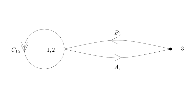
Figure 3: The gauge theory quiver for the theory after the first “step” of the RG flow. The VEV of the field $C_{3}$ breaks $SU(N)_{1}\times SU(N)_{2}$ down to $SU(N)_{1,2}$ and the massive fields $A_{1,2}$ and $B_{1,2}$ are integrated out. At the second step, node 3 confines.

This theory, however, is not conformal anymore, since we now have $N_{\rm f}=N_{\rm c}$ for the 3d node on the quiver on Fig. (3). The theory flows to the strongly coupled region and the right node confines. Apart from the adjoint fields $C_{1}$ and $C_{2}$ we have a meson $M=A_{3}B_{3}$, which also transforms in the adjoint of the left node of the quiver diagram. The field content, therefore, exactly reproduces the ${\cal N}=4$ SYM theory. The superpotential, however, involves an additional non-perturbative Affleck-Dine-Seiberg term:

$$W=\frac{1}{v}{\rm Tr}\left(M\left[C_{1},C_{2}\right]\right)+X({\rm det}M-B\tilde{B}-\Lambda^{2N}).$$ (5.6)

Here $B$ and $\tilde{B}$ are the baryon fields, $\Lambda$ is the strong coupling scale and the chiral field $X$ is the Lagrange multiplier imposing the quantum moduli constraint in the parentheses. In the deformed conifold model this constraint exhibits two completely separated branches of solutions [31, 32], since the meson and the baryons cannot acquire VEVs simultaneousely. In the present model the two branches are not separated. This, however, does not modify the observation that the superpotential is still cubic. For instance, the “purely” mesonic branch corresponds to $B=\tilde{B}=0$ and ${\rm det}M=\Lambda^{2N}$, which can solved by $M=\mathbf{1}_{N\times N}\Lambda^{2}$. Substituting this into (5.6) we find that the superpotential vanishes, so, similar to what we did in the unresolved case, we have to consider next to the leading order corrections. We will set:

$$M=\mathbf{1}_{N\times N}\Lambda^{2}+\frac{\Phi}{v},$$ (5.7)

reproducing eventually the ${\cal N}=4$ superpotential:

$$W={\rm Tr}\left(\Phi\left[C_{1},C_{2}\right]\right).$$ (5.8)

6 Discussion

In this paper we have constructed a supergravity solution that describes an RG flow from the gauge theory dual to $AdS_{5}\times S^{5}/{\mathbb{Z}}_{3}$, to ${\cal N}=4$ SYM theory which in turn is dual to $AdS_{5}\times S^{5}$. The resolution of the ${\mathbb{Z}}_{3}$ singularity is given by a ${\mathbb{C}}{\mathbb{P}}^{2}$ placed at the tip of the cone. From the explicit metric that we wrote down, it can be checked [39] that far away in the UV, the leading order correction from AdS describes an order six operator acquiring VEV in the gauge theory. This VEV is nothing but the resolution parameter in the geometry. The explicit form of this operator unfortunately is unknown.

The problem of constructing a 10$d$ supergravity background based on the resolved 6$d$ space reduces to finding the six-dimensional Green function, which serves as a warp function in the full solution. If the function, however, is taken to depend only on the radial coordinate, and so the D$3$-brane source is “smeared” over the ${\mathbb{C}}{\mathbb{P}}^{2}$, the total 10$d$ solution proves to be singular. This is just a common phenomenon for 10$d$ backrounds based on “smeared” D-branes. To avoid the singularity we have placed the D$3$ branes stuck at a point of the ${\mathbb{C}}{\mathbb{P}}^{2}$. The map between the D$3$ branes coordinates and the gauge invariant (mesonic) combination of the fields was presented in Section 3.

Back in the dual gauge theory, this corresponds to giving VEVs to some bi-fundamental fields. Although the precise form of the dimension six operator dual to the resolution parameter remains a mystery, we are able to show that there are only two distinct ways in which the fields can acquire non-trivial VEVs. In both cases the non-trivial VEVs break the $SU(3)$ isometry, the conformal invariance of the original theory and trigger (presumably) different RG flows to the same ${\cal N}=4$ SYM theory.

We have argued that in the second scenario the RG flow proceeds in two “steps”. First, some fields acquire VEVs breaking three gauge groups down to two. Integrating the massive fields out, we are left with four (two adjoints and two bi-fundamentals) out of nine original fields and a quartic superpotential. Second, one of the nodes confines. In terms of the two adjoint fields and a new meson constructed from the two bi-fundamentals, the superpotential becomes cubic like in the ${\cal N}=4$ SYM theory. It is very tempting, therefore, to identify these two steps on the supergravity side. Unfortunately, it does not look possible if one wants to stick with the supergravity approximation, which requires large t’Hooft coupling $\lambda=Ng_{YM}^{2}$. Indeed, the strong coupling scale on the second “step” of the RG flow is related to the energy scale $E$ set by the VEV $v$ as:

$$\Lambda=Ee^{-\frac{8\pi^{2}}{2Ng_{YM}^{2}(E)}}\qquad{\rm where}\qquad E=\sqrt{v}.$$ (6.1)

We see that, for large $\lambda=Ng_{YM}^{2}$ the scale $\Lambda$ and $E$ are of the same order and we cannot distinguish between them. This situation is actually familiar from the conifold model cascade [32], where on the supergravity side the cascade steps are “smoothed” out for the same reasons as in our case.

A number of interesting questions can be raised for further investigation. In [12] the presence of the baryonic VEV was verified from the analysis of the DBI action of an Euclidian D$3$-brane wrapped on a 4$d$ cycle of the resolved conifold. Similar computation can also be performed in our case. Remarkably, from the gauge theory point of view this condensate has to be the same in both suggested RG flow scenarios. Indeed, the baryon constructed from the field $A_{3}B_{3}$ and the baryon built from $C_{3}$ describe the same baryonic operator, since their product can be written only in terms of the meson $A_{3}B_{3}C_{3}$. This, and the fact that the Fayet-Iliopoulos parameters (3.7-3.9) turn out to be identical for both these choices, leads us to speculate that perhaps the two RG flows are dual descriptions of each other.

Finally, it will be very interesting to find the dimension six operator dual to the resolution parameter $a$. We hope that our paper might provide useful results towards this direction, along the lines of [39].

7 Acknowledgments

We would like to thank Riccardo Argurio, Cyril Closset and Carlo Maccaferri for helpful discussions. This work is supported in part by IISN - Belgium (convention 4.4505.86), by the Belgian National Lottery, by the European Commission FP6 RTN programme MRTN-CT-2004-005104 in which the authors are associated with V. U. Brussel, and by the Belgian Federal Science Policy Office through the Interuniversity Attraction Pole P5/27.

Appendix

A.  Metric on the ALE space

One way to derive the metric on the resolution of ${\mathbb{C}}^{3}/{\mathbb{Z}}_{3}$ is to use the fact that the Kähler form $K(r)$ on this space depends only on $r^{2}=|w_{1}|^{2}+|w_{2}|^{2}+|w_{3}|^{2}$. Since the space is Calabi-Yau, among other things, it is both Rici-flat and Kähler. So the metric can be written as $g_{i\bar{j}}=\partial_{i}\partial_{\bar{j}}K$, and then the Ricci-flatness condition turns out to be a differential equation for $K(r)$:

$${\rm det}(\partial_{i}\partial_{\bar{j}}K)={\rm const.}$$ (A.1)

After absorbing the irrelevant constant by rescaling $K(r)$, this translates to

$$(K^{\prime})^{2}(r^{2}K^{\prime\prime}+K^{\prime})=1.$$ (A.2)

The primes here are with respect to $r^{2}$. It will prove convenient to introduce a new function ${\cal F}$ defined by

$${\cal F}\equiv r^{2}K^{\prime},$$ (A.3)

in terms of which the differential equation above has the simple solution

$${\cal F}=(r^{6}+a^{6})^{1/3},$$ (A.4)

with $a^{6}$ an integration constant which reflects the resolution of the space. By tuning $a$ to zero, we can recover the unresolved space. It is easy to integrate ${\cal F}$ once again to obtain an explicit expression for $K(r)$ in terms of hypergeometric functions, but we will not need it, so we will refrain from writing it down.

Using these, and the angular variables defined in section 4 in terms of the $w_{i}$, we can calculate the metric directly as $ds^{2}=g_{i\bar{j}}dw^{i}d{\bar{w}}^{\bar{j}}$. The result is

$$ds^{2}={\cal F}^{\prime}dr^{2}+\frac{{\cal F}^{\prime}r^{2}}{9}\big{(}d\psi-\frac{3}{2}\sin^{2}\sigma(d\beta+\cos\theta d\phi)\big{)}^{2}+\hskip 122.85876pt$$

$$\hskip 43.36243pt+{\cal F}\Big{(}d\sigma^{2}+\frac{1}{4}\sin^{2}\sigma(d\theta^{2}+\sin^{2}\theta d\phi^{2})+\frac{1}{4}\sin^{2}\sigma\cos^{2}\sigma(d\beta+\cos\theta d\phi)^{2}\Big{)}.$$ (A.5)

This turns into the metric presented in Section 4, once we make the definition $\rho^{2}\equiv{\cal F}$.

B.  The Scalar Laplacian

In this appendix we exhibit the full Laplacian for the resolved ${\mathbb{C}}^{3}/{\mathbb{Z}}_{3}$ space. It takes the form

$$\Box H=\Big{(}1-\frac{a^{6}}{\rho^{6}}\Big{)}^{1/2}\partial_{\rho}\Big{(}\big{(}1-\frac{a^{6}}{\rho^{6}}\big{)}^{1/2}\partial_{\rho}H\Big{)}+\frac{1}{\rho}\Big{(}5-\frac{2a^{6}}{\rho^{6}}\Big{)}\partial_{\rho}H+\hskip 36.135pt$$

$$+\frac{1}{\rho^{2}}\Big{[}\big{(}\partial_{\sigma}^{2}H+2(\cot\sigma+\cot 2\sigma)\partial_{\sigma}H\big{)}+\frac{4}{\sin^{2}\sigma\sin\theta}\partial_{\theta}(\sin\theta\partial_{\theta}H)+\hskip 14.45377pt$$

$$+\frac{4}{\sin^{2}\sigma}\Big{(}\frac{1}{\sin\theta}\partial_{\phi}-\cot\theta\partial_{\beta}\Big{)}^{2}H+\frac{4}{\cos^{2}\sigma}\Big{(}\frac{3}{2}\sin\sigma\partial_{\psi}+\frac{1}{\sin\sigma}\partial_{\beta}\Big{)}^{2}H+$$

$$+9\Big{(}1-\frac{a^{6}}{\rho^{6}}\Big{)}^{-1}\partial_{\psi}^{2}H\Big{]}.\hskip 144.54pt$$ (B.6)

C.  Branes on the Unresolved ${\mathbb{C}}^{3}/{\mathbb{Z}}_{3}$: Away from the Tip

Here we compute the Green’s function for a D-brane stack on the unresolved orbifold, but away from the tip ($\rho\neq a$). Far away from the stack, we expect to reproduce the behavior we calculated in section 3.1, but we also expect to see the AdS throat in the near-horizon region because the stack is no longer at a singular point. The fact that the space is unresolved will be reflected in the fact that the solution is still singular.

To simplify the computations, we will look at the case where the stack is at the point $\rho=\rho_{0},\ \sigma=0$. The location $\sigma=0$ kills the dependence of the Green function on the other angles of the ${\mathbb{C}}{\mathbb{P}}^{2}$ as was argued in the main body of the paper. We will only be interested in the case where the solution is of the form $H(\rho,\sigma)$, which means that we are assuming that the D3-branes are smeared over the $\psi$-circle. The form of the Laplacian permits such a choice. The equation to be solved takes the form

$$\Box_{\rho}H+\frac{1}{\rho^{2}}\Box_{\sigma}H=\frac{-3C}{4\pi^{3}\rho^{5}\sin^{3}\sigma\cos\sigma}\delta(\rho-\rho_{0})\delta(\sigma),$$ (C.7)

$${\rm where}\ \ \Box_{\rho}=\frac{1}{\rho^{5}}\frac{\partial}{\partial\rho}\Big{(}\rho^{5}\frac{\partial}{\partial\rho}\Big{)},\hskip 54.2025pt\ \$$

with $\Box_{\sigma}$ as defined by (4.6). As before, we now solve

$$\Big{(}\Box_{\sigma}+2l(2l+4)\Big{)}\Sigma(\sigma)=0,$$ (C.8)

for the angular part in terms of Jacobi polynomials. The full normalized angular solutions are

$$Y_{l}(\sigma)=\sqrt{4(l+1)}P_{l}^{(0,1)}(-\cos 2\sigma).$$ (C.9)

The remaining radial part of the equation looks like

$$\frac{\partial^{2}H_{l}}{\partial\rho^{2}}+\frac{5}{\rho}\frac{\partial H_{l}}{\partial\rho}-\frac{2l(2l+4)}{\rho^{2}}H_{l}=\frac{-3C}{4\pi^{3}\rho^{5}}\delta(\rho-\rho_{0}),$$ (C.10)

whose solution, after matching the function and its derivative through the delta function is

$$H_{l}(\rho,\rho_{0})=\left\{\begin{array}[]{ll}\displaystyle{\frac{3C}{16\pi^{3}(l+1)}\rho_{0}^{-(2l+4)}\rho^{2l}}&\ \ \rho\leq\rho_{0},\\ \\ \displaystyle{\frac{3C}{16\pi^{3}(l+1)}\rho^{-(2l+4)}\rho_{0}^{2l}}&\ \ \rho\geq\rho_{0}.\\ \end{array}\right.$$ (C.14)

The full solution looks like

$$H(\rho,\rho_{0};\sigma,0)=\sum_{l}H_{l}(\rho,\rho_{0})Y_{l}^{*}(0)Y_{l}(\sigma).$$ (C.15)

Restricting to $l=0$ gives the dependence far away from the source

$$H(\rho)\rightarrow\frac{3C}{16\pi^{3}\rho^{4}}\times\big{(}\sqrt{4}\ \big{)}^{2}=\frac{12\pi g_{s}N\alpha^{\prime 2}}{\rho^{4}}$$ (C.16)

which reproduces the result obtained in section 3.1, eqn. (3.5), where the stack was assumed to be at the tip. The emergence of the AdS throat close to the stack is entirely analogous to the resolved case, which was discussed in the main text.

D.  Warp Factor with Smeared Sources

In this appendix, we compute the warp factor for the resolved ${\mathbb{C}}^{3}/{\mathbb{Z}}_{3}$, but with the assumption that the source branes are smeared all over the resolution and there is no angular dependence. We start with the Laplacian as defined by

$$\Box H=\frac{1}{\sqrt{g_{6}}}\ \partial_{\mu}(\sqrt{g_{6}}g^{\mu\nu}\partial_{\nu}H)=\frac{1}{\rho^{5}}\partial_{\rho}\Big{(}\rho^{5}\big{(}1-\frac{a^{6}}{\rho^{6}}\big{)}\partial_{\rho}H\Big{)}$$ (D.17)

where we have used (4.5) and assumed $H\equiv H(\rho)$, which is the basis of the smeared source approximation. For comparison with the unsmeared solution in the main body of the paper, we will solve the Green’s equation in terms of $r=(\rho^{6}-a^{6})^{1/6}$. The equation is effectively first order and can be solved by direct integration in terms of elementary functions. But we will write its solution in a hypergeometric form

$$H=\frac{12\pi g_{s}N\alpha^{\prime 2}}{r^{4}}\ {}_{2}F_{1}\Big{(}\frac{2}{3},\ \frac{2}{3};\ \frac{5}{3};-\frac{a^{6}}{r^{6}}\Big{)},$$ (D.18)

for ease of comparison. We have fixed the overall normalization by demanding that the warp-function should look like that of the unresolved case (3.5), far away from the resolution ($\frac{a}{r}\rightarrow 0$).

E.  The Mass Matrix for the Unresolved Case

We have argued above that the VEVs $A_{3}=B_{3}=C_{3}=v$ render the superpotential quadratic in terms of the remaining fields and the symmetric mass matrix $\mathbf{M}$ has rank four. In this appendix we present the basis in which the mass matrix acquires a diagonal form. In the $(A_{1},A_{2},B_{1},B_{2},C_{1},C_{2})$ basis we have:

$$\mathbf{M}=\frac{v}{2}\left(\begin{array}[]{cccccc}0&0&0&0&1&-1\\ 0&0&0&-1&0&1\\ 0&0&0&1&-1&0\\ 0&-1&1&0&0&0\\ 1&0&-1&0&0&0\\ -1&1&0&0&0&0\end{array}\right).$$

The matrix eigenvalues are $0$, $\frac{\sqrt{3}}{2}v$ and $-\frac{\sqrt{3}}{2}v$. Each of the eigenvalues has degeneracy two. The corresponding eigenvectors are as follows:

$$\left(\begin{array}[]{c}\frac{1}{\sqrt{3}}\\ \frac{1}{\sqrt{3}}\\ \frac{1}{\sqrt{3}}\\ 0\\ 0\\ 0\end{array}\right)\quad\left(\begin{array}[]{c}0\\ 0\\ 0\\ \frac{1}{\sqrt{3}}\\ \frac{1}{\sqrt{3}}\\ \frac{1}{\sqrt{3}}\end{array}\right)\quad\left(\begin{array}[]{c}\frac{1}{\sqrt{3}}\\ -\frac{1}{2\sqrt{3}}\\ -\frac{1}{2\sqrt{3}}\\ 0\\ \frac{1}{2}\\ -\frac{1}{2}\end{array}\right)\quad\left(\begin{array}[]{c}0\\ -\frac{1}{2}\\ \frac{1}{2}\\ \frac{1}{\sqrt{3}}\\ -\frac{1}{2\sqrt{3}}\\ -\frac{1}{2\sqrt{3}}\end{array}\right)\quad\left(\begin{array}[]{c}\frac{1}{\sqrt{3}}\\ -\frac{1}{2\sqrt{3}}\\ -\frac{1}{2\sqrt{3}}\\ 0\\ -\frac{1}{2}\\ \frac{1}{2}\end{array}\right)\quad\left(\begin{array}[]{c}0\\ \frac{1}{2}\\ -\frac{1}{2}\\ \frac{1}{\sqrt{3}}\\ -\frac{1}{2\sqrt{3}}\\ -\frac{1}{2\sqrt{3}}\end{array}\right)$$ (E.19)

References

- [1] I. R. Klebanov and E. Witten, Superconformal field theory on threebranes at a Calabi-Yau singularity, Nucl. Phys. B 536, 199 (1998) [arXiv:hep-th/9807080].
- [2] J. M. Maldacena, The large N limit of superconformal field theories and supergravity, Adv. Theor. Math. Phys. 2, 231 (1998) [Int. J. Theor. Phys. 38, 1113 (1999)] [arXiv:hep-th/9711200].
- [3] D. R. Morrison and M. R. Plesser, Non-spherical horizons. I, Adv. Theor. Math. Phys. 3, 1 (1999) [arXiv:hep-th/9810201].
- [4] V. Bouchard, Lectures on complex geometry, Calabi-Yau manifolds and toric geometry, arXiv:hep-th/0702063.
- [5] K. Hori et al., Mirror symmetry, Providence, USA: AMS (2003) 929 p.
- [6] W. Fulton, Introduction to toric varieties, Annals of Mathematical Studies, Princeton University Press, 1993, 157 p.
- [7] B. Ezhuthachan, S. Govindarajan and T. Jayaraman, Fractional two-branes, toric orbifolds and the quantum McKay correspondence, JHEP 0610, 032 (2006) [arXiv:hep-th/0606154].
- [8] E. Witten, Phases of N = 2 theories in two dimensions, Nucl. Phys. B 403, 159 (1993) [arXiv:hep-th/9301042].
- [9] P. Candelas and X. C. de la Ossa, Comments on Conifolds, Nucl. Phys. B 342, 246 (1990).
- [10] S. Gukov, M. Rangamani and E. Witten, Dibaryons, strings, and branes in AdS orbifold models, JHEP 9812, 025 (1998) [arXiv:hep-th/9811048].
- [11] I. R. Klebanov and E. Witten, AdS/CFT correspondence and symmetry breaking, Nucl. Phys. B 556, 89 (1999) [arXiv:hep-th/9905104].
- [12] I. R. Klebanov and A. Murugan, Gauge/gravity duality and warped resolved conifold, JHEP 0703, 042 (2007) [arXiv:hep-th/0701064].
- [13] L. A. Pando Zayas and A. A. Tseytlin, 3-branes on resolved conifold, JHEP 0011, 028 (2000) [arXiv:hep-th/0010088].
- [14] S. G. Nibbelink, M. Trapletti and M. Walter, Resolutions of C**n/Z(n) orbifolds, their U(1) bundles, and applications to string model building, JHEP 0703, 035 (2007) [arXiv:hep-th/0701227].
- [15] O. J. Ganor and J. Sonnenschein, On the strong coupling dynamics of heterotic string theory on C**3/Z(3), JHEP 0205, 018 (2002) [arXiv:hep-th/0202206].
- [16] J. P. Gauntlett, D. Martelli, J. Sparks and D. Waldram, Sasaki-Einstein metrics on S(2) x S(3), Adv. Theor. Math. Phys. 8, 711 (2004) [arXiv:hep-th/0403002].
- [17] T. Eguchi, P. B. Gilkey and A. J. Hanson, Gravitation, Gauge Theories And Differential Geometry, Phys. Rept. 66, 213 (1980).
- [18] A. Lukas and S. Morris, Moduli Kaehler potential for M-theory on a G(2) manifold, Phys. Rev. D 69, 066003 (2004) [arXiv:hep-th/0305078].
- [19] M. R. Douglas and G. W. Moore, D-branes, Quivers, and ALE Instantons, arXiv:hep-th/9603167.
- [20] M. R. Douglas, B. R. Greene and D. R. Morrison, Orbifold resolution by D-branes, Nucl. Phys. B 506, 84 (1997) [arXiv:hep-th/9704151].
- [21] B. Feng, A. Hanany and Y. H. He, D-brane gauge theories from toric singularities and toric duality, Nucl. Phys. B 595, 165 (2001) [arXiv:hep-th/0003085].
- [22] K. D. Kennaway, Brane Tilings, Int. J. Mod. Phys. A 22, 2977 (2007) [arXiv:0706.1660 [hep-th]].
- [23] S. Kachru and E. Silverstein, 4d conformal theories and strings on orbifolds, Phys. Rev. Lett. 80, 4855 (1998) [arXiv:hep-th/9802183].
- [24] F. Bigazzi, A. L. Cotrone, M. Petrini and A. Zaffaroni, Supergravity duals of supersymmetric four dimensional gauge theories, Riv. Nuovo Cim. 25N12, 1 (2002) [arXiv:hep-th/0303191].
- [25] C. E. Pearson, Handbook of Applied Mathematics: Selected Results and Methods, Van Nostrand Reinhold, (1983) 1307 p.
- [26] http://functions.wolfram.com/HypergeometricFunctions/Hypergeometric2F1/17/02/07/
- [27] http://functions.wolfram.com/Polynomials/JacobiP/23/01/0003/index.html
- [28] http://en.wikipedia.org/wiki/Bessel_function
- [29] R. Argurio, M. Bertolini, S. Franco and S. Kachru, Gauge/gravity duality and meta-stable dynamical supersymmetry breaking, JHEP 0701, 083 (2007) [arXiv:hep-th/0610212].
- [30] R. Argurio, M. Bertolini, S. Franco and S. Kachru, Metastable vacua and D-branes at the conifold, JHEP 0706, 017 (2007) [arXiv:hep-th/0703236].
- [31] I. R. Klebanov and A. A. Tseytlin, Gravity duals of supersymmetric SU(N) x SU(N+M) gauge theories, Nucl. Phys. B 578, 123 (2000) [arXiv:hep-th/0002159].
- [32] I. R. Klebanov and M. J. Strassler, Supergravity and a confining gauge theory: Duality cascades and chiSB-resolution of naked singularities, JHEP 0008, 052 (2000) [arXiv:hep-th/0007191].
- [33] A. Butti, D. Forcella, A. Hanany, D. Vegh and A. Zaffaroni, Counting Chiral Operators in Quiver Gauge Theories, JHEP 0711, 092 (2007) [arXiv:0705.2771 [hep-th]].
- [34] W. Chen, M. Cvetic, H. Lu, C. N. Pope and J. F. Vazquez-Poritz, Resolved Calabi-Yau Cones and Flows from Superconformal Field Theories, Nucl. Phys. B 785, 74 (2007) [arXiv:hep-th/0701082].
- [35] H. Singh, 3-Branes on Eguchi-Hanson 6D Instantons, arXiv:hep-th/0701140.
- [36] M. Cvetic and J. F. Vazquez-Poritz, Warped Resolved Cones, arXiv:0705.3847 [hep-th].
- [37] D. Martelli and J. Sparks, Baryonic branches and resolutions of Ricci-flat Kahler cones, arXiv:0709.2894 [hep-th].
- [38] I. R. Klebanov, A. Murugan, D. Rodriguez-Gomez and J. Ward, Goldstone Bosons and Global Strings in a Warped Resolved Conifold, arXiv:0712.2224 [hep-th].
- [39] S. Benvenuti, M. Mahato, L. A. Pando Zayas and Y. Tachikawa, The gauge / gravity theory of blown up four cycles, arXiv:hep-th/0512061.
- [40] M. Bertolini, F. Bigazzi and A. L. Cotrone, New checks and subtleties for ads/cft and a-maximization, [arXiv:hep-th/0411249].
- [41] S. Benvenuti, S. Franco, A. Hanany, D. Martelli and J. Sparks, An infinite family of superconformal quiver gauge theories with Sasaki-Einstein duals, [arXiv:hep-th/0411264].
- [42] M. Cvetic, H. Lu, D. N. Page and C. N. Pope, New Einstein-Sasaki spaces in five and higher dimensions, [arXiv:hep-th/0504225].
- [43] S. Benvenuti and M. Kruczenski, Semiclassical strings in Sasaki-Einstein manifolds and long operators in N = 1 gauge theories, [arXiv:hep-th/0505046].
- [44] S. Benvenuti and M. Kruczenski, From Sasaki-Einstein spaces to quivers via BPS geodesics: , [arXiv:hep-th/0505206].
- [45] S. Franco, A. Hanany, D. Martelli, J. Sparks, D. Vegh and B. Wecht, Gauge theories from toric geometry and brane tilings, [arXiv:hep-th/0505211].
- [46] M. Cvetic, H. Lu, D. N. Page and C. N. Pope, New Einstein-Sasaki and Einstein spaces from Kerr-de Sitter, [arXiv:hep-th/0505223].
- [47] D. Martelli and J. Sparks, Toric Sasaki-Einstein metrics on , [arXiv:hep-th/0505027].
- [48] D. Berenstein, C. P. Herzog, P. Ouyang and S. Pinansky, Supersymmetry breaking from a Calabi-Yau singularity, [arXiv:hep-th/0505029].
- [49] S. Franco, A. Hanany, F. Saad and A. M. Uranga, Fractional branes and dynamical supersymmetry breaking, [arXiv:hep-th/0505040].
- [50] M. Bertolini, F. Bigazzi and A. L. Cotrone, Supersymmetry breaking at the end of a cascade of Seiberg dualities, [arXiv:hep-th/0505055].
- [51] J. Evslin, C. Krishnan and S. Kuperstein, Cascading Quivers from Decaying D-branes, JHEP 0708, 020 (2007) [arXiv:0704.3484 [hep-th]].
- [52] D. Martelli and J. Sparks, Toric geometry, Sasaki-Einstein manifolds and a new infinite class of AdS/CFT duals, [arXiv:hep-th/0411238].
- [53] C. P. Herzog, Q. J. Ejaz and I. R. Klebanov, Cascading RG flows from new Sasaki-Einstein manifolds, [arXiv:hep-th/0412193].
- [54] B. A. Burrington, J. T. Liu, M. Mahato and L. A. Pando-Zayas, Towards supergravity duals of chiral symmetry breaking in Sasaki-Einstein cascading quiver theories, [arXiv:hep-th/0504225].
- [55] D. Gepner and S. S. Pal, Branes in L(p,q,r), [arXiv:hep-th/0505039].