Spectra of accretion discs around white dwarfs

Abstract

We present spectra of accretion discs around white-dwarfs calculated with an improved and updated version of the Shaviv & Wehrse (1991) model. The new version includes line opacities and convective energy transport and can be used to calculate spectra of hot discs in bright systems (nova–like variables or dwarf novae in outburst) as well as spectra of cold accretion discs in quiescent dwarf novae.

1 Introduction

In weakly magnetized cataclysmic variable stars (CVs) matter lost by a Roche-lobe filling low-mass companion forms an accretion disc around the white-dwarf primary. In bright systems such as nova-like binaries and dwarf-novae in outburst the disc is the dominant source of luminosity but even in quiescence the disc emission might provide crucial information about the physics of accretion, in particular about the mechanisms transporting angular momentum and releasing gravitational energy.

Until now one could calculate only spectra for hot accretion discs (see Wade & Hubeny, 1998, and references therein). In such an approach the disc is divided into rings whose vertical structure is calculated using the program TLUSDISK Hubeny (1990, 1991). A different way of solving radiative transfer equations in accretion discs was presented by Shaviv & Wehrse (1991, hereafter SW). Also, in their approach one could apply it to hot discs only. The preliminary attempt to apply the SW code to cold quiescent discs in Idan et al. (1999) was not conclusive. The main obstacle in solving the vertical structure of cold accretion discs is the presence of convection-dominated zones. (The description of the quiescent disc of SS Cyg by Kromer et al., 2007, neglects convection).

The absence of spectral models for cold quiescent discs is the reason why fitting models to observations can be a frustrating exercise(see Urban & Sion, 2006, and references therein). Using the models of hot stationary discs of Wade & Hubeny (1998) to describe the spectra of cold (and non-stationary) quiescent discs cannot be expected to give relevant results. In fact since the observational data were the UV spectra obtained by the IUE, it was not very surprising that the best fits were obtained with no disc emission at all: quiescent discs are not supposed to be UV emitters so that the only source of UV radiation in such systems should be the white dwarf.

The description of the quiescent state of the dwarf-nova cycle is the Achilles heel of the widely accepted disc instability model (DIM) according to dwarf-nova outbursts are due to a thermal-viscous instability (see Lasota, 2001, for a review). For example while the DIM predicts the quiescent disc to be optically thick (especially in its outer regions), the observations of the quiescent dwarf-nova IP Peg seem to suggest the opposite (Littlefair et al., 2001; Ribeiro et al., 2007). Correct modeling of the emission from quiescent discs is therefore an obvious prerequisite to solving this thorny problem .

In general a full description of dwarf-nova outburst cycle should include the radiation transfer equations. In practice this much too costly and therefore unfeasible. However, instead of including one can combine the DIM with the solutions of the radiative transfer equations for the same disc parameters. The Hameury et al. (1998, hereafter HMDLH) version of the DIM in which the time-dependent radial evolution equations use as input a pre-calculated grid of hydrostatic vertical structures (a 1+1D scheme) is well suited to such enterprize. The vertical structures are calculated using the standard equations of stellar structure or the grey-atmosphere approximation in the optically thin case. The angular-momentum viscosity transport mechanism is described by the $\alpha$-ansatz of Shakura & Sunyaev (1973). For a given $\alpha$, $M/R^{3}$ and effective temperature $T_{\mathrm{eff}}$ there exist a unique solution describing the disc vertical structure. Such solutions which are very handy for solving the time-dependent equations of the disc evolution cannot be used to produce emission spectra. These can be, however, calculated by using the same input parameters ($\alpha$, $M/R^{3}$ and $T_{\mathrm{eff}}$) in a radiative-transfer code on the condition that the vertical solutions calculated by the two methods are the same. In this way one can reproduce spectra of the whole cycle of a dwarf-nova outburst.

The outline of the present article is as follows. In section 2 we discuss the model used with special stress put on marking the differences with original SW code on which it has been based. In section 3 we present solutions obtained for various types of physical set-ups. In subsection 3.2 we compare our solutions for vertical structure with those obtained with HMDLH code. Then in 3.5 we compare our disc spectra with the UV spectra obtained by Wade & Hubeny (1998). In the following subsection subsec:non-stat we present spectra of cold non-equilibrium discs which in the DIM represent the quiescent state of the dwarf-nova outburst cycle. Section 4 contains the discussion, and conclusion.

2 Assumptions, equations and methods of solution

The structure of the code is based on the model of Shaviv & Wehrse (1991). The principal improvements consist in using (modern) line opacities and in a different treatment of the convective energy transport. It seems that our code is the only working accretion-disc radiative-transfer code which includes convection self-consistently and is able to handle dominant convective fluxes.

2.1 Assumptions

The accretion disc is described as composed of concentric rings orbiting the central gravitating body of mass $M$ with the Keplerian angular frequency

$$\Omega_{\rm K}=\sqrt{\frac{GM}{R^{3}}}.$$ (1)

We assume that the disc is geometrically thin, i.e.

$$z_{0}\ll R$$ (2)

where $z_{0}$ is the disc height. This assumption allows to decompose the disc equations into their vertical and radial components. In this paper we will solve only the vertical accretion-disc equations and obtain the corresponding emission spectra. However, since the radiation of a steady-state accretion disc can be considered as a sum of radiation from individual rings our results can directly applied to such configurations. The same is true of quasi-stationary phases of dwarf-nova outbursts. Also radiation from non-steady quiescent discs of dwarf-nova stars can be treated as being the sum of the emission of individual rings. This is true as long as radial gradients are much smaller than the vertical ones. During the outburst of dwarf nova when the temperature and densities fronts are propagating through the disc this assumption might no longer be valid.

2.2 Equations

The vertical structure of a ring at a distance $R$ from the center is found by solving:

• The hydrostatic equilibrium equation

  $$\frac{dP}{dz}=-\rho\,g_{z}=-\rho\,\Omega_{K}\,z,$$ (3)

• The energy balance equation

  $$\frac{dF_{\rm z}}{dz}=Q_{\rm vis}=\left(\frac{dF_{\rm z}}{dz}\right)_{\rm rad}+\left(\frac{dF_{\rm z}}{dz}\right)_{\rm conv},$$ (4)

  where $F_{\rm z}$ is the energy flux in the vertical ($z$) direction. We use the $\alpha$ prescription of Shakura & Sunyaev (1973) to describe the viscous energy generation

  $$Q_{\rm vis}(z,R)=\frac{3}{2}\alpha\Omega_{\rm K}\frac{P}{\rho}.$$ (5)

• The radiative energy flux is given by

  $$\begin{array}[t]{r}\int_{0}^{\infty}\,\left(J(z,R,\lambda)-B(T(z,R),\lambda)\right)\kappa(\lambda)d\lambda\\ =-Q_{\rm vis}(z,R)\end{array}$$ (6)

  where $J$ is the mean intensity, $B$ the Planck function and $\kappa(\lambda)$ is the monochromatic mass absorption coefficient.

• The radiative transfer equation is

  $$\mathbf{n}\cdot\mathbf{{\nabla}}I=\kappa(S-I),$$ (7)

  where $I$ is the intensity, $S$ the source function and $\mathbf{n}$ is a unit vector in the ray direction.

• Following HMDLH the convective energy flux is calculated by the method of Paczyński (1969).

  Whenever the radiative gradient

  $$\nabla_{\rm rad}\equiv\left(\frac{d\ln T}{d\ln P}\right)_{\rm rad}$$ (8)

  is superadiabatic, the temperature gradient of the structure $\nabla$ is convective ($\nabla=\nabla_{\rm conv}$). The convective gradient is calculated in the mixing length approximation, with the mixing length taken as $H_{\rm ml}=\alpha_{\rm ml}H_{P}$, where $H_{P}$ is the pressure scale height:

  $$H_{P}={P\over\rho g_{\rm z}+(P\rho)^{1/2}\Omega_{\rm K}},$$ (9)

  The convective gradient is found from:

  $$\nabla_{\rm conv}=\nabla_{\rm ad}+(\nabla_{\rm rad}-\nabla_{\rm ad})Y(Y+A)$$ (10)

  where $\nabla_{\rm ad}$ is the adiabatic gradient, and $Y$ is the solution of the cubic equation:

  $${9\over 4}{\tau_{\rm ml}^{2}\over 3+\tau_{\rm ml}^{2}}Y^{3}+VY^{2}+V^{2}Y-V=0$$ (11)

  where $\tau_{\rm ml}=\kappa\rho H_{\rm ml}$ is the optical depth of the convective eddies. It is assumed that the eddies are optically thick so that the convection is efficient, yet the contribution to the adiabatic gradient $\nabla_{\rm ad}+(\nabla_{\rm rad}-\nabla_{\rm ad})Y(Y+A)$ cannot be neglected. In those cases in which the convection reached the photosphere the effect on the weak lines must be noticeable. The coefficient $V$ is given by:

  $$V^{-2} = \left({3+\tau_{\rm ml}^{2}\over 3\tau_{\rm ml}}\right)^{2}{g_{\rm z}^{2}H_{\rm ml}^{2}\rho^{2}C_{P}^{2}\over 512\sigma^{2}T^{6}H_{P}}$$ (12)

  $$\hskip 30.00005pt\times\left({\partial\ln\rho\over\partial\ln T}\right)_{P}(\nabla_{\rm rad}-\nabla_{\rm ad})$$

  In our model we take $\alpha_{\rm ml}=1.5$

• The outer boundary condition is

  $$Q_{\rm vis}=\sigma T_{\rm eff}^{4}$$ (13)

  In the case of a stationary disc

  $$\dot{M}=2\pi R\int_{0}^{Z_{0}}\rho v_{r}dz=constant,$$ (14)

  where $v_{r}$ is the radial flow velocity one has

  $$Q_{\rm vis}=\frac{3}{8\pi\sigma}\left(\frac{GM_{\rm wd}\dot{M}}{R^{3}}\right)\left(1-\left(\frac{R_{wd}}{R}\right)^{1/2}\right)$$ (15)

  but our solutions apply to any distribution of accretion rate $\dot{M}(r)$ in a geometrically thin accretion disc.

2.3 Input (opacities and EOS)

We have improved several features of the original SW code but the use of modern opacities and especially of the line opacities is the major improvement that we present here in some detail.

There are several ways of calculating opacities. They can be obtained using either codes such as PHOENIX (Hauschildt et al., 1999), “Atlas 12” (Kurucz, 1992) or from the database of the OP project (Seaton et al., 1994). The updated version of the SW code can use the opacities from “Atlas 12” but since calculating the opacities is time consuming we decided to use tabulated data from the OP database. To tabulate the data we used the data from the Opacity Project - $OPCD\_3.3$ that were downloaded from the website at the Centre des Donnés de Strasbourg (CDS). For a given abundance mixture the subroutines $mx.f$, $mixv.f$, $opfit.f$ and $mixz.f$ allowed us (with some modifications) getting the tabulated opacities for the wavelengths chosen as our basic grid. For the emerging spectra from every ring we use 10,000 wavelengths starting from $100$Å up to $10^{6}$Å. The grid interval varies between $\Delta\lambda=0.25$Å for the most important zone such as the range between $850-2300$Å and $1-2$Å used for wavelengths shorter than $800$Å or above $2300$Å. For wavelengths longer than $5000$Å, $\Delta\lambda$ varies logarithmicaly starting at $2$Å and getting up to $200$Å for the very long wavelengths. All the data were tabulated using a grid for the temperature $T$ and electron density $Ne$. The indices $ite$ and $jne$ are defined by

$$\begin{array}[t]{l}ite=40x\log(T),\ \ jne=4x\log(Ne)\\ \triangle(ite)=\triangle(jne)=2\end{array}$$ (16)

The mesh in the tables is calculated for $140<ite<320$ therefore the lowest temperature that can be used in the code is $3160\rm K$. Let us stress that the opacities in the present work do NOT take into account the global line broadening due effects such as velocities, (expansion opacity, see Shaviv & Wehrse, 2005), the inclination of the disc or microscopic such as microturbulence. Consequently, the lines provide only an indication of the presence of a given ion and cannot be used, so far, for abundance determinations etc. These broadenings will be included in the code in the near future. Therefore the results presented here should be treated as more qualitative than quantitative in the sense that for the moment we will not discuss the ratios between the emission or absorption lines but rather their presence or absence in the spectrum.

The reason for allowing the code to work either with OP tabulated data or with “Atlas 12” was to test the tabulated opacities. In Figure 1 we show the comparison of opacities as function of wavelength calculated for $T=10^{5}$K and $\rho=2\times 10^{-8}$ g cm^-3, and $T=3\times 10^{4}$K and $\rho=2\times 10^{-7}$g cm^-3 using either “Atlas 12” or the OP. The “Atlas 12” continuum opacities used were for a solar mixture with the addition of only H and He lines. The opacities from the OP Project are for also for mixture of solar abundance (which includes the lines and the continuum).

The Rosseland mean opacities are taken from OPAL tables for solar composition. While solving the radiative transfer equation we checked for the consistency between the Rosseland mean opacity obtaining from the solution of the radiative transfer equation and the value from the OPAL table. The equation of state is interpolated from the tables of Fontaine & Graboske & Van Horn (1977). The equation of state used in the OP project is different than the one use by Kurucz or in OPAL. We are aware of the this problem and its effect on the opacities but we will not discussed it here.

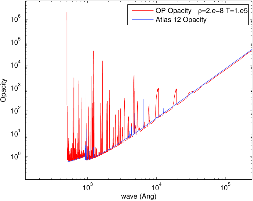
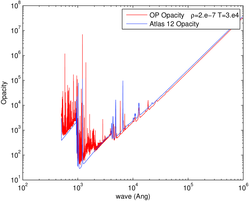
Figure 1: Comparision between the opacities as function of wavelength obtained from Atlas 12 and those obtain from the OP for T= and $\rho=$ (upper figure) and T= and $\rho=$ (lower figure). The Atlas 12 opacities are the continuum opacities with only H and He lines, while the OP opacities are for solar mixture

2.4 The method of solution

The basic idea behind the SW code was to couple the hydrostatic with the radiative-transfer equations. Therefore the code iterates the two equations simultaneously. The iteration continues until a structure is found to which both the solution for the hydrostatic and the radiative-transfer equations converge.

The temperature profile is determined from Eq. (6). The temperature $T(z,R)$ in this equation is solved by expressing $J$ in terms of $B$ using the radiative transfer equation (for detail description see Kalkofen & Wehrse (1984),Wehrse (1981)). As mentioned above we assumed that each radial ring is independent of its neighboring rings hence there is only a vertical radiative flux. The radiative transfer equation is solved in the two stream approximation. $I^{+}$ represent the specific intensity in the outward direction and $I^{-}$ is the specific intensity in the inward direction. The radiative equation is then written as:

$$\pm\frac{dI^{\pm}(R,z,\lambda)}{dz} = -(\kappa(\lambda)+\sigma(\lambda))I^{\pm}(R,z,\lambda)$$

$$+ \sigma(\lambda)J(R,z,\lambda)+\kappa(\lambda)B(T(R,z),\lambda)$$

where $\sigma(\lambda)$ is the scattering coefficient. We use the same N grid points as in the hydrostatic calculation. The boundary conditions are: no incident flux ($I^{-}_{j,1}=0$) and at the equatorial plane the upward and downward specific intensities are equal ($I^{+}_{j,N}=I^{-}_{j,N}$), where j designates the ring number.

When solving the vertical-structure equations of an accretion disc the main problem is that contrary to stellar atmospheres the exact height of the photosphere is unknown a-priori. Because of gravity increasing with height a change in the position of the photosphere is followed by a change of the gravitational acceleration which leads to a change in the entire vertical structure of the disc. One has to remember that the upper part of the disc is optically thin and may include, depending on the assumptions, a non negligible energy production. However, since this optically thin region is a poor radiator and absorber a small energy production there might have large effect on the final temperature structure. Once the line opacities are taken into account the importance of tuning the disc height is crucial since otherwise the outgoing radiative flux might not be equal to the total energy flux of the ring. Consequently the great sensitivity of the emission lines to the details of the temperature at the edge of the photosphere might be used to investigate the properties of the energy-release (“viscosity”) mechanism.

In view of the above we approach the problem in the following way: we guess first an initial temperature–optical depth relation and assume an initial height $z_{0}$. The optical depth in the disc uppermost point is chosen to be $10^{-6}$, and this assumption is checked again once the final structure is obtained. With the help of the T($\tau$) relation we can integrate the hydrostatic equation from $z_{0}$ down to $z=0$. One should emphasize that $\tau$ in the current work is the Rosseland mean and not the optical depth at 5000Å as in SW. When the height $z_{0}$ is the correct height, the total energy generation rate in the ring calculated from the energy equation is equal to the total luminosity of that particular ring. If this is not the case we alter $z_{0}$ keeping the T($\tau$) relation fixed, until the this condition is satisfied. Once this iteration is solved the hydrostatic model is consistent with the energy generation but not yet with the radiation field.

We then turn to solving the radiative transfer equation using the disc height, the pressure and the density structure obtained from the hydrostatic iteration. This structure is kept fixed during the iteration for the radiative field. We now solve the radiative transfer equation and obtain a new $T(\tau)$ relation, where new values of the temperature are assigned to old values of the optical depth. If the new $T(\tau)$ relation from the radiative iteration agrees (to a chosen degree of accuracy) with the old $T(\tau)$ relation from the hydrostatic iteration the hydrostatic structure is consistent with the radiation field. If not we iterate again with the new $T(\tau)$ relation.

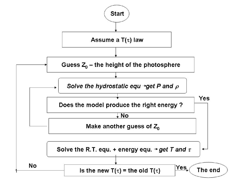
Figure 2: The iteration scheme

To summarize we have 3 basic iteration loops (see figure 2) in the code :

1. Calculating the hydrostatic structure using a given $T(\tau)$ relation. The output results are the disc height, pressure and density structure.

2. Solving the radiative transfer for a given disc height, P and $\rho$. The output result is a new $T(\tau)$ relation.

3. Repeating the previous two iterations until the $T(\tau)$ relation from the hydrostatic part is equal to the $T(\tau)$ relation from the radiative transfer equation.

Only after these iterations converge the emerging flux from the disc is calculated using the radiative transfer equation.

As mentioned before the entire disc is divided into a series of concentric rings and their width is determined according to their distance from the WD. All rings which are further away than $2\mbox{$R_{\mathrm{wd}}$}$ are assumed to have a width of $1\mbox{$R_{\mathrm{wd}}$}$, below $2\mbox{$R_{\mathrm{wd}}$}$ the width of the ring is taken to be $0.05\mbox{$R_{\mathrm{wd}}$}$, which allows a detailed calculation of the emission of the rings near the boundary layer.

The vertical structure of the ring itself is divided into 100 $z$ points (100 layers) and we use 10000 wavelengths. The above procedure is repeated for each ring. The emerging fluxes from the rings are then integrated in order to get the total flux from the entire disc according to:

$$F_{\rm total}=\int_{\mbox{$R_{\mathrm{in}}$}}^{\mbox{$R_{\mathrm{out}}$}}F(R)RdR$$ (18)

3 Results

3.1 Comparison with HMDLH vertical structures

As we mention in the introduction a 1+1D scheme was developed by HMDLH to describe the time-dependent evolution of the dwarf nova outbursts. The scheme uses as input a pre-calculated grid of hydrostatic vertical structures. For a given $\alpha$, $M/R^{3}$ and effective temperature $T_{\mathrm{eff}}$ there exist a unique solution describing the vertical structure of a disc in thermal equilibrium. HMDLH code cannot be used to produce emission spectra. These can be, however, calculated by using the same input parameters ($\alpha$, $M/R^{3}$ and $T_{\mathrm{eff}}$) in the present code (hereafter ILHS) on the condition that the vertical solution calculated by the two methods are the same. In this way one can reproduce spectra of almost the whole cycle of a dwarf-nova outburst. This procedure makes sense only if the structures calculated by the two methods are practically the same.

In order to compare the solutions obtained by HMDLH with those calculated with ILHS we show in Figures 3 and 4 the vertical structures for hot and cold discs with effective temperatures $15000$K and $5000$K respectively. The mass of the white dwarf is $0.6M_{\odot}$, the ring radius is $5\mbox{$R_{\mathrm{wd}}$}$ where the white dwarf radius was calculated according to Nauenberg (1972) mass-radius relation.We used two values of the viscosity parameter $\alpha=0.03$ and $0.3$. One sees a perfect agreement for the $\alpha=0.3$, while the minor differences for the $\alpha=0.03$ are of the order of $3\%$.

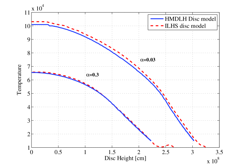
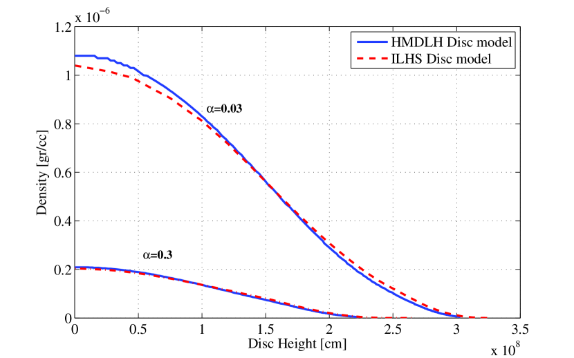
Figure 3: Comparison between the temperature and density profile at R=5$R_{\mathrm{wd}}$ and $T_{\mathrm{eff}}$=$15000$K calculated by the HMDLH disc model and the present disc model taking into account the radiative transfer equation for $\alpha=0.3$ and $\alpha=0.03$.

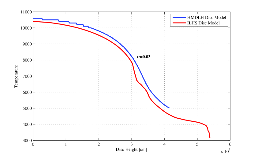
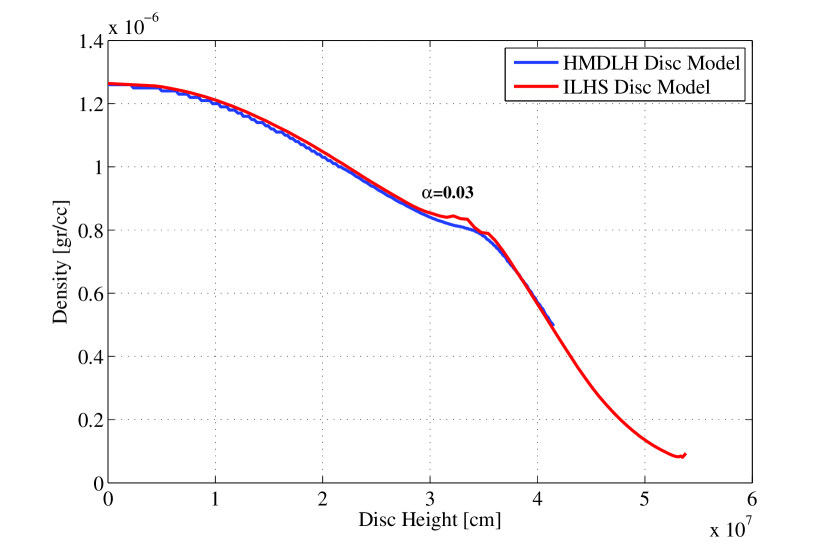
Figure 4: Comparison between the temperature and density profile at R=5$R_{\mathrm{wd}}$ and $T_{\mathrm{eff}}$=$5000$K, $\alpha=0.03$ calculated by the HMDLH disc model and the present disc model taking into account the radiative transfer equation.

3.2 S-curves

For a given mass and distance from the center the thermal equilibria of accretion discs can be represented as a $T_{\rm eff}(\Sigma)$-relation. These equilibria forms an S shape on the $(\Sigma,T_{\rm eff})$ plane. Figure 5 shows an example‘s of $\Sigma-\mbox{$T_{\mathrm{eff}}$}$ S curves obtained with both the HMDLH code and the radiative-transfer calculation of the ILHS. $\alpha$ is constant and the radius is $5R_{\rm wd}$. Each point on the S-curve represents a thermal-equilibrium at that radius. The upper branch of the S-curve is the hot stable branch, while the lower branch where the temperature is below $\simeq 6000$K, represent the cold stable solutions. The middle branch of the S-curve corresponds to thermally unstable equilibria.

The agreement between the two codes is very good especially on the upper branch of the S-Curve. However, the disc at the lower turning knee of the S-curve (in the unstable zone) is fully convective. Here we were unable to calculate the structure with the full radiative transfer equation code. The degree of accuracy that was chosen for the $T-\tau$ to converge in these calculations was $1\%$. But since near the lower turning knee of the S-curve the disc is almost completely convective and any small change in the initial conditions such as the initial optical depth will affect the structure of the disc, we assume that the acceptable error are of the order of few percent. The agreement between the two codes on the lower stable branches of the S-curve is very good.

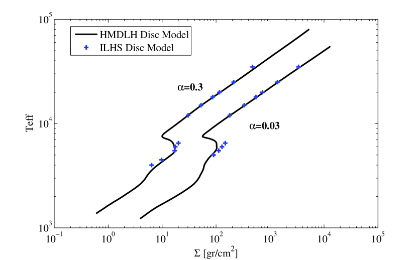
Figure 5:  $\Sigma-\mbox{$T_{\mathrm{eff}}$}$ curves for $R=\mbox{$R_{\mathrm{wd}}$}$, $\mbox{$M_{\mathrm{wd}}$}=0.6\mbox{$\mathrm{M_{\odot}}$}$, and $\alpha=0.03$ and 0.3. The solid line is the HMDLH model while + represent the results from the ILHS disc calculation.

3.3 The single ring spectrum

In Figures 6, 7 and 8 we present the spectra obtained from single-ring calculations at $\mbox{$R_{\mathrm{wd}}$}=5\mbox{$\mathrm{R_{\odot}}$}$ for $\mbox{$M_{\mathrm{wd}}$}=0.6\mbox{$\mathrm{M_{\odot}}$}$. The spectra (in arbitrary units) were calculated for a cold disc with $\alpha=0.03$ $\mbox{$T_{\mathrm{eff}}$}=5000$K and a hot disc with $\alpha=0.3$, $\mbox{$T_{\mathrm{eff}}$}=15000$K. The spectrum of the cold disc is dominated by narrow emission lines while the spectrum of the hot disc is dominated by wide absorption line. In the hot disc spectrum (8) we can identify the Balmer lines (the $4100{\AA},4340{\AA},4860{\AA}$ lines). The absorption lines have various structures : in some cases such as the Lyman lines or the $H_{\gamma}$ line in hot disc, there is an emission line in the center of the absorption line. We should emphasize again that one must be careful when interpreting the results at this point, since in this paper the opacities do not include line broadening and are not taking into account the Gaussian instrumental broadening function that affects and smears most of the fine lines. Such broadening can change or even eliminate some of the fine structure of the lines that is seen in the figures.

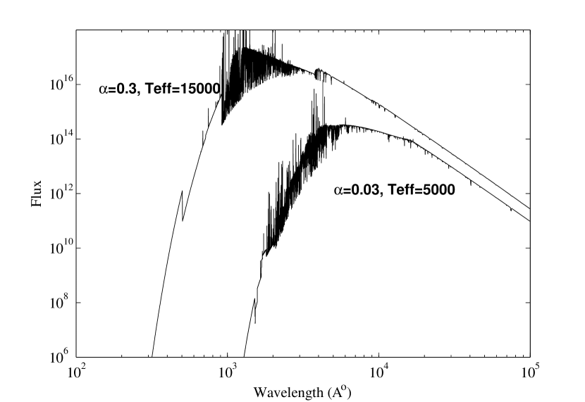
Figure 6: The spectra obtained from a single-ring calculation for cold ($\alpha=0.3$,$\mbox{$T_{\mathrm{eff}}$}=15000$K) and hot disc ($\alpha=0.03,\mbox{$T_{\mathrm{eff}}$}=5000$K). The ring parameters are $\mbox{$R_{\mathrm{wd}}$}=5\mbox{$\mathrm{R_{\odot}}$}$ and $\mbox{$M_{\mathrm{wd}}$}=0.6\mbox{$\mathrm{M_{\odot}}$}$.

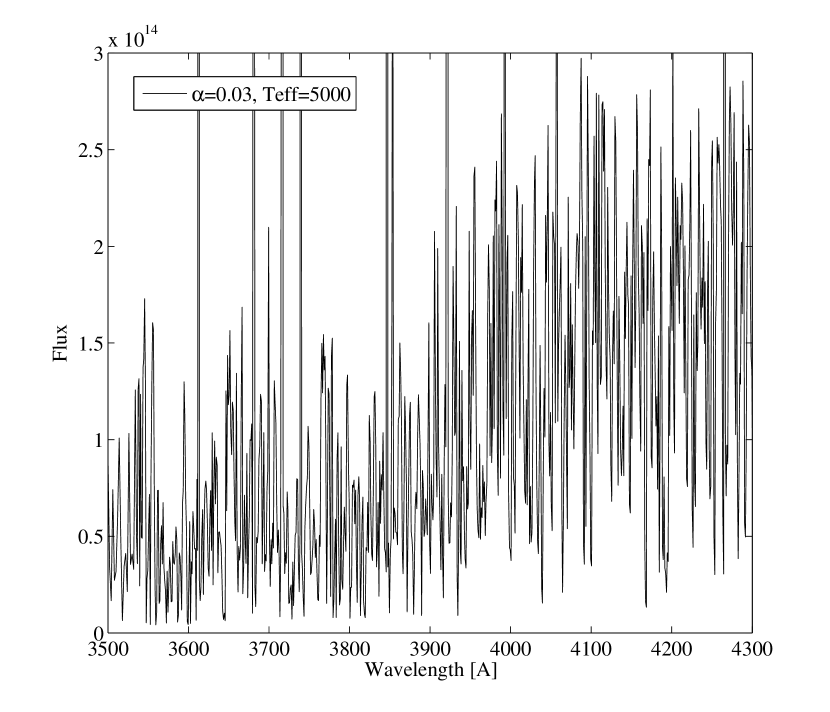
Figure 7: The flux at the wavelength between $3500-4000$Å, for cold disc ($\alpha=0.03,\mbox{$T_{\mathrm{eff}}$}=5000$K). The spectrum is dominated by emission lines.

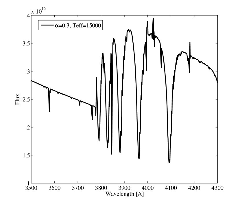
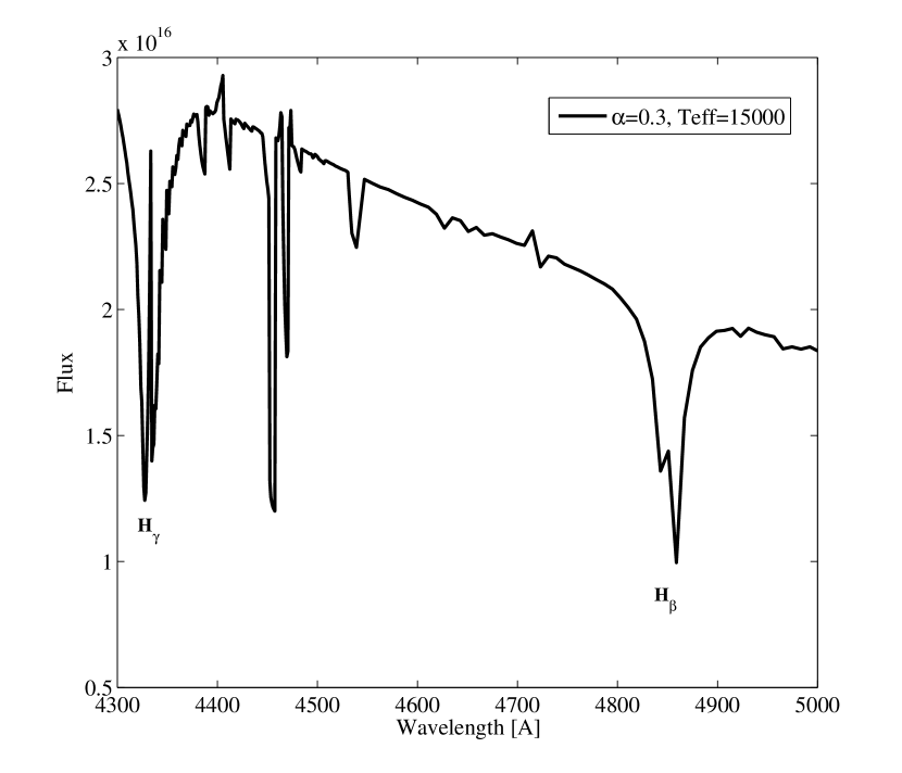
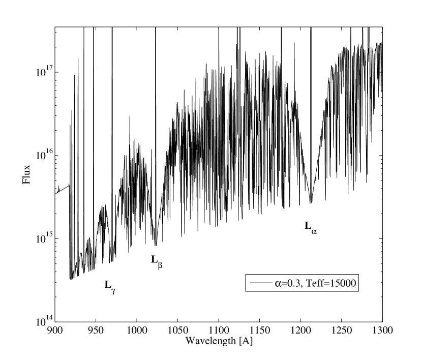
Figure 8: The flux as function of wavelength, for hot disc ($\alpha=0.3,\mbox{$T_{\mathrm{eff}}$}=15000$K). The spectrum is dominated by absorption lines and in some cases narrow emission line in the central of the absorption “well”

3.4 Stationary disc solutions for high accretion rates and $\alpha=0.3$

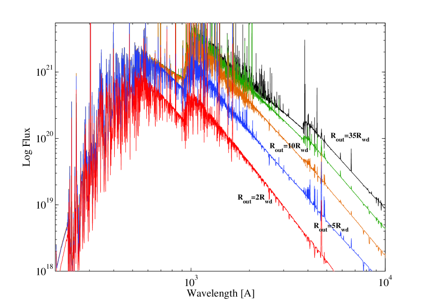
Figure 9: The integrated disc spectrum as function of the disc radii for a hot disc $\alpha=0.3,\mbox{$M_{\mathrm{wd}}$}=0.8\mbox{$\mathrm{M_{\odot}}$}$

In Figures 9 we present an example for the total spectrum of a hot disc $\alpha=0.3,\mbox{$M_{\mathrm{wd}}$}=0.8\mbox{$\mathrm{M_{\odot}}$}$ and accretion rate of $10^{17}\rm g\,s^{-1}$. We show spectra for increasing disc area - from the inner part of the disc (the inner $2\mbox{$R_{\mathrm{wd}}$}$ area) up to the largest outer radius calculated - $35\mbox{$R_{\mathrm{wd}}$}$. One can clearly see the different area in the disc in which different type of emission is formed. For example: the Balmer jump which will dominate the total flux from the disc is formed on the outer part of the disc, while the inner part of the disc is dominated only by few absorption lines.

3.5 Comparison with Wade & Hubeny hot accretion disc spectra

Wade & Hubeny (1998, hereafter WH) calculated a large grid of far- and mid-ultraviolet spectra (850-2000 Å) of the integrated light from steady-state accretion disks in bright cataclysmic variables. All their models are for disc atmospheres which are optically thick and are viewed from a distance of $100\rm pc$.

Figure 10 shows a comparison between a WH accretion disc spectrum (model cc) and a spectrum obtained with our model. The model parameters were are: $\mbox{$M_{\mathrm{wd}}$}=0.8\mbox{$\mathrm{M_{\odot}}$}$ and $\log\dot{M}=-8.5\mbox{$\mathrm{M_{\odot}}$}\rm y^{-1}$. In our disc model we used and the same number of rings as in their paper. The viscosity prescription in WH is different from the $\alpha$ ansatz used in our model. Their viscosity is based on Reynolds number approach ($\rm K\check{r}\acute{\i}\check{z}$ & Hubeny, 1986) . A value of $Re=5000$ was assumed for all radii. We estimated that $\alpha=0.3$ corresponds to the parameters of WH model cc.

WH spectra are smoother than our spectra since their models have been convolved with a Gaussian instrumental profile but one can expect that in our spectrum most of the narrow emission lines will disappear after such convolution. In general both spectra are similar.

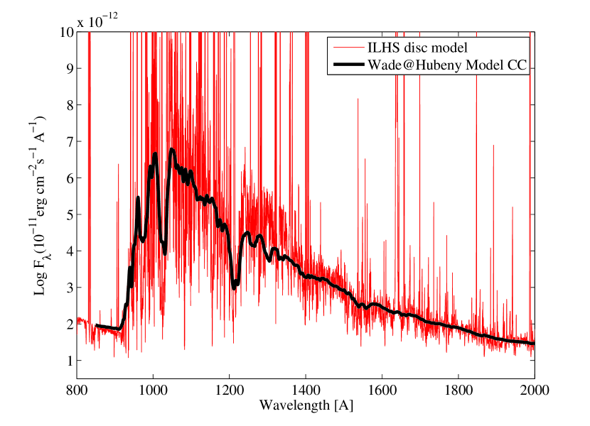
Figure 10: Comparison between Wade and Hubeny model cc spectrum (thick black line) and the spectrum from our disc model (grey line) for $\alpha=0.3$ and $\log\dot{M}=-8.5\mbox{$\mathrm{M_{\odot}}$}\rm yr^{-1}$.

3.6 Quiescent dwarf-nova disc: on-stationary solution $\alpha=0.03$, $\mbox{$T_{\mathrm{eff}}$}=5000$.

Dwarf-nova quiescent discs are non-stationary, i.e. $\mbox{$\dot{M}$}\neq constant$ since they are filling-up getting ready for the next outburst. The whole disc must be cold, its temperature everywhere must be lower than the critical instability temperature. In general, for most of the quiescence the temperature profile is roughly flat. We modeled as an example the spectrum of such a disc assuming $\mbox{$T_{\mathrm{eff}}$}=5000$K (which is a bit high for a real disc since the critical temperature is close to that value).

The total flux for an outer radius of $25\mbox{$R_{\mathrm{wd}}$}$ is shown in figure 11. The spectrum between $3000-10000$Å is nearly a flat as observed, no Balmer jump is present. As can be seen from figure 11 for this particular calculation, there is no contribution from the disc spectrum in the UV range.

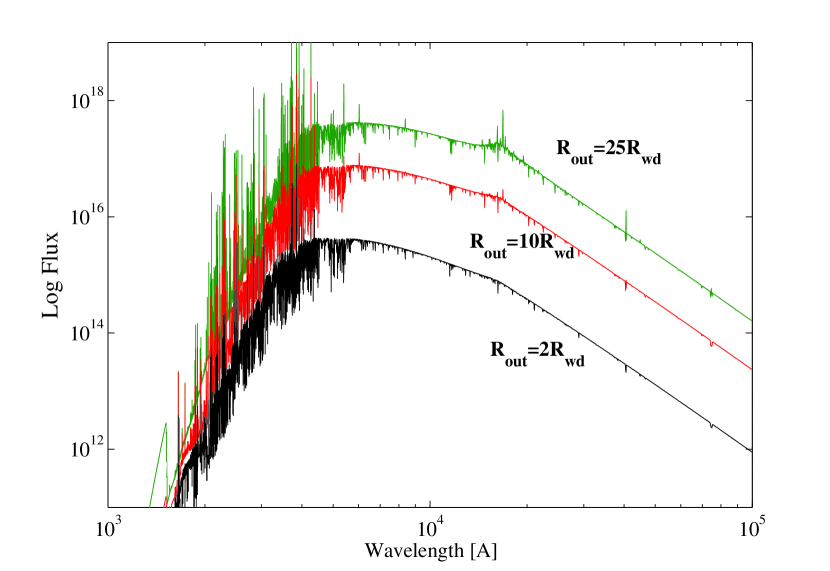
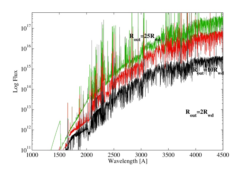
Figure 11: The integrated disc spectrum as function of the disc radii for a cold disc $\alpha=0.03,\mbox{$T_{\mathrm{eff}}$}=5000\mbox{$M_{\mathrm{wd}}$}=0.6\mbox{$\mathrm{M_{\odot}}$}$

4 Future work

In the future we will produce a grid of disc spectra will be used to make comparisons between observations and the model spectra. In particular will focus on the quiescence disc and the effect of the irradiation by the white dwarf and the formation of a corona. Combining ILHS with the time dependent HMDLH code will provide a tool to study the dwarf nova outburst cycle.

The variations in the shapes of selected lines that are formed in different parts of the disc will be studied with the purpose to develop spectral-disc-tomography.

References

- Fontaine & Graboske & Van Horn (1977) Fontaine, G., & Graboske, H.C. Jr. & Van Horn H.M. 1977, ApJS, 35, 293
- Hameury et al. (1998) Hameury, J.-M., Menou, K., Dubus, G., Lasota, J. -P., & Huré, J.M. 1998, MNRAS, 298, 1048
- Hauschildt et al. (1999) Hauschildt, P. H., Allard, F., Ferguson, J., Baron, E., & Alexander, D. R. 1999, ApJ, 525, 871
- Hubeny (1990) Hubeny, I. 1990, ApJ, 351, 632
- Hubeny (1991) Hubeny, I. 1991, IAU Colloq. 129: The 6th Institute d’Astrophysique de Paris (IAP) Meeting: Structure and Emission Properties of Accretion Disks, 227
- Idan et al. (1999) Idan, I., Lasota, J.-P., Hameury, J.-M., & Shaviv, G. 1999, Phys. Rep., 311, 213
- Kalkofen & Wehrse (1984) Kalkofen W., Wehrse, R., 1984 Methods in radiative transfer, W. Kalkofen, ed. Cambridge University Press, 307.
- & Hubeny (1986) , S., & Hubeny, I. 1986, Bull. Astron. Inst. Czechoslovakia, 37, 129.
- Kromer et al. (2007) Kromer, M., Nagel, T., & Werner, K. 2007, A&A, 475, 301
- Kurucz (1992) Kurucz, R. L. 1992, Revista Mexicana de Astronomia y Astrofisica, vol. 23, 23, 45
- Lasota (2001) Lasota, J.-P. 2001, New Astronomy Review, 45, 449
- Littlefair et al. (2001) Littlefair, S. P., Dhillon, V. S., Marsh, T. R., & Harlaftis, E. T. 2001, MNRAS, 327, 475
- Nauenberg (1972) Nauenberg M., 1972, ApJ, 175, 417
- Orosz & Wade (2003) Orosz, J. A., & Wade, R. A. 2003, ApJ, 593, 1032
- Paczyński (1969) Paczyński B., 1969, Acta Astronomica, 19, 1
- Ribeiro et al. (2007) Ribeiro, T., Baptista, R., Harlaftis, E. T., Dhillon, V. S., & Rutten, R. G. M. 2007, A&A, 474, 213
- Seaton et al. (1994) Seaton, M. J., Yan, Y., Mihalas, D., & Pradhan, A. K. 1994, MNRAS, 266, 805
- Shakura & Sunyaev (1973) Shakura, N.I., Sunyaev, R.A., 1973 A&A, 24, 337,
- Shaviv & Wehrse (1991) Shaviv, G., Wehrse, R., 1991 A&A, 251, 117,
- Shaviv & Wehrse (2005) Shaviv, G., Wehrse, R., 2005 A&A, 440, 13,
- Urban & Sion (2006) Urban, J. A., & Sion, E. M. 2006, ApJ, 642, 1029
- Wade & Hubeny (1998) Wade, R.A., Hubeny, I., 1998 ApJ, 509, 350,
- Wehrse (1981) Wehrse, R., 1981 MNRAS, 195, 553,
- Warner (1995) Warner, B. 1995, Cataclysmic Variable Stars (Cambridge: Cambridge University Press)