Thermodynamical properties of the ICM from hydrodynamical simulations

Abstract

Modern hydrodynamical simulations offer nowadays a powerful means to trace the evolution of the X–ray properties of the intra–cluster medium (ICM) during the cosmological history of the hierarchical build up of galaxy clusters. In this paper we review the current status of these simulations and how their predictions fare in reproducing the most recent X–ray observations of clusters. After briefly discussing the shortcomings of the self–similar model, based on assuming that gravity only drives the evolution of the ICM, we discuss how the processes of gas cooling and non–gravitational heating are expected to bring model predictions into better agreement with observational data. We then present results from the hydrodynamical simulations, performed by different groups, and how they compare with observational data. As terms of comparison, we use X–ray scaling relations between mass, luminosity, temperature and pressure, as well as the profiles of temperature and entropy. The results of this comparison can be summarised as follows: (a) simulations, which include gas cooling, star formation and supernova feedback, are generally successful in reproducing the X–ray properties of the ICM outside the core regions; (b) simulations generally fail in reproducing the observed “cool core” structure, in that they have serious difficulties in regulating overcooling, thereby producing steep negative central temperature profiles. This discrepancy calls for the need of introducing other physical processes, such as energy feedback from active galactic nuclei, which should compensate the radiative losses of the gas with high density, low entropy and short cooling time, which is observed to reside in the innermost regions of galaxy clusters.

1 Introduction

Clusters of galaxies form from the collapse of exceptionally high density perturbations having typical size of $\sim 10$ Mpc in a comoving frame. As such, they mark the transition between two distinct regimes in the study of the formation of cosmic structures. The evolution of structures involving larger scales is mainly driven by the action of gravitational instability of the dark matter (DM) density perturbations and, as such, it retains the memory of the initial conditions. On the other hand, galaxy–sized structures, which form from initial fluctuations on scales of $\sim 1$ Mpc, evolve under the combined action of gravity and of complex gas–dynamical and astrophysical processes. On such scales, gas cooling, star formation and the subsequent release of energy and metal feedback from supernovae (SN) and active galactic nuclei (AGN) have a deep impact on the observational properties of the diffuse gas and of the galaxy population.

In this sense, clusters of galaxies can be used as invaluable cosmological tools and astrophysical laboratories (see Rosati et al. 2002 and Voit 2005 for reviews). These two aspects are clearly interconnected with each other. From the one hand, the evolution of the population of galaxy clusters and their overall baryonic content provide in principle powerful constraints on cosmological parameters. On the other hand, for such constraints to be robust, one has to understand in detail the physical properties of the intra–cluster medium (ICM) and its interaction with the galaxy population.

The simplest model to predict the properties of the ICM and their evolution has been proposed by Kaiser (1986). This model is based on the assumption that the evolution of the thermodynamical properties of the ICM is determined only by gravity, with gas heated to the virial temperature of the hosting DM halos by accretion shocks (Bykov et al. 2008 - Chapter 7, this volume). Since gravitational interaction does not introduce any preferred scale, this model has been called “self–similar”. As we shall discuss, this model provides precise predictions on the shape and evolution of scaling relations between X–ray luminosity, entropy, total and gas mass, which have been tested against numerical hydrodynamical simulations (e.g., Eke et al. 1998; Bryan & Norman 1998). These predictions have been recognised for several years to be at variance with a number of observations. In particular, the observed relation between X–ray luminosity and temperature (e.g. Markevitch 1998; Arnaud & Evrard 1999; Osmond & Ponman 2004) is steeper and the measured level of gas entropy higher than expected (e.g., Ponman et al. 2003; Pratt & Arnaud 2005), especially for poor clusters and groups. This led to the concept that more complex physical processes, related to the heating from astrophysical sources of energy feedback, and radiative cooling of the gas in the central cluster regions, play a key role in determining the properties of the diffuse hot baryons.

Although semi–analytical approaches (e.g., Tozzi & Norman 2001; Voit 2005, and references therein) offer invaluable guidelines to this study, it is only with hydrodynamical simulations that one can capture the full complexity of the problem, so as to study in detail the existing interplay between cosmological evolution and the astrophysical processes.

In the last years, ever improving code efficiency and supercomputing capabilities have opened the possibility to perform simulations over fairly large dynamical ranges, thus allowing to resolve scales of a few kiloparsecs (kpc), which are relevant for the formation of single galaxies, while capturing the global cosmological environment on scales of tens or hundreds of Megaparsecs (Mpc), which are relevant for the evolution of galaxy clusters. Starting from first attempts, in which only simplified heating schemes were studied (e.g., Navarro et al. 1995; Bialek et al. 2001; Borgani et al. 2002), a number of groups have studied the effect of introducing also cooling (e.g. Katz & White 1993; Lewis et al. 2000; Muanwong et al. 2001; Davé et al. 2002; Tornatore et al. 2003), of more realistic sources of energy feedback (e.g., Borgani et al. 2004; Kay et al. 2007; Nagai et al. 2007a; Sijacki et al. 2007), of thermal conduction (e.g., Dolag et al. 2004), and of non–thermal pressure support from magnetic fields (e.g., Dolag et al. 2001) and cosmic rays (e.g., Pfrommer et al. 2007).

In this paper, we will review the recent advancement performed in this field of computational cosmology and critically discuss the comparison between simulation predictions and observations, by restricting the discussion to the thermal effects. As such, this paper complements the reviews by Borgani et al. 2008 - Chapter 18, this volume, which reviews the study of the ICM chemical enrichment and by Dolag et al. 2008b - Chapter 15, this volume, which reviews the study of the non–thermal properties of the ICM from simulations. We refer to the reviews by Dolag et al. 2008a - Chapter 12, this volume for a description of the techniques of numerical simulations and by Kaastra et al. 2008 - Chapter 9, this volume for an overview of the observed thermal properties of the ICM.

The scheme of the presentation is as follows. In Sect. 2 we briefly discuss the self–similar model of the ICM and how the action of non–gravitational heating and cooling are expected to alter the predictions of this model. Sect. 3 and 4 overview the results obtained on the comparison between observed and simulated scaling relations and profiles of X–ray observable quantities, respectively. In Sect. 5 we summarise and critically discuss the results presented.

2 Modelling the ICM

2.1 The self–similar scaling

The simplest model to predict the observable properties of the ICM is based on the assumption that gravity only determines the thermodynamical properties of the hot diffuse gas (Kaiser 1986). Since gravity does not have preferred scales, we expect clusters of different sizes to be the scaled version of each other. This is the reason why this model has been called self-similar.

If, at redshift $z$, we define $M_{\Delta_{\displaystyle{\rm c}}}$ to be the mass contained within the radius $r_{\Delta_{\displaystyle{\rm c}}}$, encompassing a mean density $\Delta_{\rm c}$ times the critical density $\rho_{\rm c}(z)$, then $M_{\Delta_{\displaystyle{\rm c}}}\propto\rho_{\rm c}(z)\Delta_{\rm c}r_{\Delta_{\displaystyle{\rm c}}}^{3}$. The critical density of the universe scales with redshift as $\rho_{\rm c}(z)=\rho_{\rm c0}E^{2}(z)$, where $E(z)$ is given by

$$E(z)\,=\,\left[(1+z)^{3}\Omega_{\rm m}+(1+z)^{2}\Omega_{\rm k}+\Omega_{\Lambda}\right]^{1/2}\,,$$ (1)

where $\Omega_{\rm m}$ and $\Omega_{\Lambda}$ are the density parameters associated to the non–relativistic matter and to the cosmological constant, respectively, $\Omega_{\rm k}=1-\Omega_{\rm m}-\Omega_{\Lambda}$ and we neglect any contribution from relativistic species.

Therefore, the cluster size $r_{\Delta_{\displaystyle{\rm c}}}$ scales with $z$ and $M_{\Delta_{\displaystyle{\rm c}}}$ as $r_{\Delta_{\displaystyle{\rm c}}}\propto M_{\Delta_{\displaystyle{\rm c}}}^{1/3}E^{-2/3}(z)$, so that, assuming hydrostatic equilibrium, cluster mass scales with temperature $T$ as

$$M_{\Delta_{\displaystyle{\rm c}}}\,\propto\,T^{3/2}E^{-1}(z)\,.$$ (2)

If $\rho_{\rm gas}$ is the gas density, the corresponding X–ray luminosity is

$$L_{X}\,=\,\int_{V}\left({\rho_{\rm gas}\over\mu m_{\rm p}}\right)^{2}\Lambda(T)\,{\rm d}V\,,$$ (3)

where $\Lambda(T)\propto T^{1/2}$ for pure thermal Bremsstrahlung emission. If gas accretes along with DM by gravitational instability during the formation of the cluster halo, then we expect that $\rho_{\rm gas}(r)\propto\rho_{\rm DM}(r)$, so that

$$L_{X}\,\propto\,M_{\Delta_{\displaystyle{\rm c}}}\rho_{\rm c}T^{1/2}\,\propto\,T^{2}E(z)\,.$$ (4)

Another useful quantity characterising the thermodynamical properties of the ICM is the entropy (Voit 2005) which, in X–ray studies of the ICM, is usually defined as

$$K\,=\,{{\rm k}_{\rm B}T\over\mu m_{\rm p}\rho_{\rm gas}^{2/3}}\,,$$ (5)

where ${\rm k}_{\rm B}$ is the Boltzmann constant, $\mu$ the mean molecular weight ($\simeq 0.58$ for a plasma of primordial composition) and $m_{\rm p}$ the proton mass. With the above definition, the quantity $K$ is the constant of proportionality in the equation of state of an adiabatic mono-atomic gas, $P=K\rho_{\rm gas}^{5/3}$. Using the thermodynamic definition of specific entropy, $s=c_{V}\ln(P/\rho_{\rm gas}^{5/3})$ ($c_{V}$: heat capacity at constant volume), one obtains $s={\rm k}_{\rm B}\ln K^{3/2}+s_{0}$, where $s_{0}$ is a constant. Another quantity, often called “entropy” in the cluster literature, which we will also use in the following, is

$$S\,=\,{\rm k}_{\rm B}Tn_{\rm e}^{-2/3}\,,$$ (6)

where $n_{\rm e}$ is the electron number density. According to the self–similar model, this quantity, computed at a fixed overdensity $\Delta_{\rm c}$, scales with temperature and redshift according to

$$S_{\Delta_{\displaystyle{\rm c}}}\propto T(1+z)^{-2}\,.$$ (7)

As already mentioned in the introduction, a number of observational facts from X–ray data point against the simple self–similar picture. The steeper slope of the $L_{X}$–$T$ relation (Markevitch 1998; Arnaud & Evrard 1999; Osmond & Ponman 2004), $L_{X}\propto T^{\alpha}$ with $\alpha\simeq 3$ for clusters and possibly larger for groups, the excess entropy in poor clusters and groups (Ponman et al. 2003; Pratt & Arnaud 2005; Piffaretti et al. 2005) and the decreasing trend of the gas mass fraction in poorer systems (Lin et al. 2003; Sanderson et al. 2003) all point toward the presence of some mechanism which significantly affects the ICM thermodynamics.

2.2 Heating and cooling the ICM

The first mechanism, that has been introduced to break the ICM self–similarity, is non–gravitational heating (e.g. Evrard & Henry 1991; Kaiser 1991; Tozzi & Norman 2001). The idea is that by increasing the gas entropy with a given extra heating energy per gas particle $E_{\rm h}$ prevents gas from sinking to the centre of DM halos, thereby reducing gas density and X–ray emissivity. This effect will be large for small systems, whose virial temperature is ${\rm k}_{\rm B}T\lesssim E_{\rm h}$, while leaving rich clusters with ${\rm k}_{\rm B}T\gg E_{\rm h}$ almost unaffected. Therefore, we expect that the X–ray luminosity and gas content are relatively more suppressed in poorer systems, thus leading to a steepening of the $L_{X}$–$T$ relation.

The notion of non–gravitational heating has been first implemented in non–radiative (i.e. neglecting the effect of cooling) hydrodynamical simulations by either injecting entropy in an impulsive way at a given redshift (Navarro et al. 1995; Bialek et al. 2001), or by adding energy in a redshift–modulated way, so as to mimic the rate of SN explosions from an external model of galaxy formation (Borgani et al. 2002). In Fig. 1 we show the different efficiency that different heating mechanisms have in breaking the self–similar behaviour of the entropy profiles in objects of different mass, ranging from a Virgo–like cluster to a poor galaxy group. According to the self–similar model, the profiles of reduced entropy, $S/T$, should be independent of the cluster mass. This is confirmed by the left panel, which also shows that these profiles have a slope consistent with that predicted by a model in which gas is shock heated by spherical accretion in a DM halo, under the effect of gravity only (Tozzi & Norman 2001). The central panel shows instead the effect of adding energy from SN, whose rate is that predicted by a semi–analytical model of galaxy formation. In this case, which corresponds to a total heating energy of about 0.3 keV/particle, the effect of extra heating starts being visible, but only for the smaller system. It is only with the pre–heating scheme, based on imposing an entropy floor of 50 keV cm², that self–similarity is clearly broken. While this heating scheme is effective in reproducing the observed $L_{X}$–$T$ relation, it produces large isentropic cores, a prediction which is at variance with respect to observations (e.g., Donahue et al. 2006).

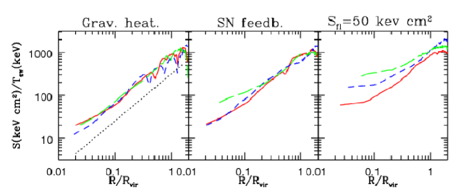
Figure 1: Profiles of reduced entropy, $S/T$, for non–radiative simulations (from Borgani et al. 2001). The left panel is for simulations including only gravitational heating, the central panel is for runs including SN feedback as predicted by a semi–analytical model of galaxy formation and the right panel is with pre–heating with an entropy threshold at redshift $z=3$. Solid, short–dashed and long–dashed curves are for a 3 keV cluster, for a 1 keV group and for a 0.5 keV group, respectively. The dotted straight line in the left panel shows the analytical prediction by Tozzi & Norman (2001) for the entropy profile associated to gravitational heating.

Although it may look like a paradox, radiative cooling has been also suggested as a possible alternative to non–gravitational heating to increase the entropy level of the ICM and suppressing the gas content in poor systems. As originally suggested by Voit & Bryan (2001), cooling provides a selective removal of low–entropy gas from the hot X–ray emitting phase (see also Wu & Xue 2002). As a consequence, while the global entropy of the baryons decreases, the entropy of the X–ray emitting gas increases. This is illustrated in the left panel of Fig. 2 (from Voit & Bryan 2001). In this plot, each of the two curves separates the upper portion of the entropy–temperature plane, where the gas has cooling time larger than the age of the system, from the lower portion, where gas with short cooling time resides. This implies that only gas having a relatively high entropy will be observed as X–ray emitting, while the low–entropy gas will be selectively removed by radiative cooling. The comparison with observational data of clusters and groups, also reported in this plot, suggests that their entropy level may well be the result of this removal of low–entropy gas operated by radiative cooling. This analytical prediction has been indeed confirmed by radiative hydrodynamical simulations. The right panel of Fig. 2 shows the results of the simulations by Davé et al. (2002) on the temperature dependence of the central entropy of clusters and groups. Quite apparently, the entropy level in simulations is well above the prediction of the self–similar model, by a relative amount which increases with decreasing temperature, and in reasonable agreement with the observed entropy level of poor clusters and groups.

Although cooling may look like an attractive solution, it suffers from the drawback that a too large fraction of gas is converted into stars in the absence of a source of heating energy which regulates the cooling runaway. Indeed, while observations indicate that only about 10 per cent of the baryon content of a cluster is in the stellar phase (e.g., Balogh et al. 2001; Lin et al. 2003), radiative simulations, like those shown in Fig. 2, convert into stars up to $\sim 50$ per cent of the gas.

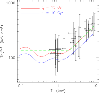
Figure 2: Left panel: the relation between entropy and temperature for gas having a fixed value of the cooling time (from Voit & Bryan 2001). The crosses with error bars are observational data on the entropy measured at one–tenth of the virial radius for clusters and groups by Ponman et al. (1999). Right panel: a comparison between observations (error bars with crosses; Ponman et al. (1999) and simulations, including radiative cooling and star formation (numbers), for the entropy in the central regions of galaxy groups and clusters. The solid line shows the prediction of the self–similar model (from Davé et al. 2002).

Another paradoxical consequence of cooling is that it increases the temperature of the hot X–ray emitting gas at the centre of clusters. This is shown in the left panel of Fig. 3 (from Tornatore et al. 2003), which compares the temperature profiles for the non–radiative run of a Virgo–like cluster with a variety of radiative runs, based on different ways of supplying non–gravitational heating. The effect of introducing cooling is clearly that of steepening the temperature profiles in the core regions, while leaving it unchanged at larger radii. The reason for this is that cooling causes a lack of central pressure support. As a consequence, gas starts flowing in sub-sonically from more external regions, thereby being heated by adiabatic compression. As we shall discuss in Sect. 4, this feature of cooling makes it quite difficult to reproduce the structure of the cool cores observed in galaxy clusters.

Steepening of the central temperature profiles and overcooling are two aspects of the same problem. In principle, the solution to this problem should be provided by a suitable scheme of gas heating which regulates star formation, while maintaining pressurised gas in the hot phase. The right panel of Fig. 3 compares the temperature–density phase diagrams for gas particles lying in the central region of an SPH–simulated cluster, when using two different feedback efficiencies. The two simulations include cooling, star formation and feedback in the form of galactic winds powered by SN explosions, following the scheme introduced by Springel & Hernquist (2003a). The upper (green) and the lower (red) clouds of high temperature particles correspond to a wind velocity of $500\,{\rm km\,s^{-1}}$ and of $1000\,{\rm km\,s^{-1}}$, respectively. This plot illustrates another paradoxical effect: in the same way that cooling causes an increase of the temperature of the hot phase, supplying energy with an efficient feedback causes a decrease of the temperature. The reason for this is that extra energy compensates radiative losses, thereby maintaining the pressure support for gas which would otherwise have a very short cooling time, thereby allowing it to survive on a lower adiabat. It is also worth reminding that cooling efficiency increases with the numerical resolution (e.g., Balogh et al. 2001; Borgani et al. 2006). Therefore, for a feedback mechanism to work properly, it should be able to stabilise the cooling efficiency in a way which is independent of resolution.

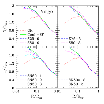
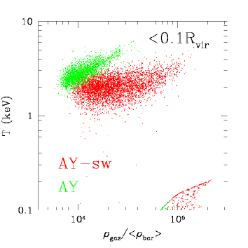
Figure 3: Left panel: temperature profiles from hydrodynamical simulations of a $\sim 3$ keV galaxy cluster. In all panels the dotted and the solid curves correspond to a non radiative run and to a run including cooling and star formation. The other curves are for different recipes of gas heating (from Tornatore et al. 2003). Right panel: the relation between temperature and overdensity for gas particles within 0.1$r_{200}$ for SPH simulations of a cluster of mass $\simeq 10^{14}\,h^{-1}{\rm M}_{\odot}$. Upper (green) points are for a run which includes feedback through galactic winds with a velocity of $500~{}\,{\rm km\,s^{-1}}$, while the lower (red) points are for a run based on assuming stronger winds (sw), with a twice as large velocity. Both runs include a model of chemical enrichment (Borgani et al. 2008 - Chapter 18, this volume) which assumes an Initial Mass Function for star formation by Arimoto & Yoshii 1987 (AY). The points in the bottom right corner are star–forming gas particles.

In the light of these results, it is clear that the observed lack of self–similarity in the X–ray properties of clusters cannot be simply explained on the grounds of a single effect. The emerging picture is that the action of cooling and of feedback energy, e.g. associated to SN explosions and AGN, should combine in a self–regulated way. As we shall discuss in the following sections, hydrodynamical simulations of galaxy clusters in a cosmological context demonstrate that achieving this heating/cooling balance is not easy and represents nowadays one of the most challenging tasks in the numerical study of clusters.

As an example, we show in Fig. 4 how the gas density of a simulated cluster changes, both at $z=2$ (left panels) and at $z=0$ (right panels), when cooling and star formation are combined with different forms of non–gravitational heating (from Borgani et al. 2005). The comparison of the top and central panels shows the effect of increasing the kinetic energy carried by galactic outflows by a factor of six. The stronger winds are quite efficient in stopping star formation in the small halos, which are washed out, and make the larger ones slightly puffier, while preserving the general structure of the cosmic web surrounding the Lagrangian cluster region. Comparing the top and the bottom panels shows instead the effect of adding to galactic winds also the effect of an entropy floor. Although the energy budget of the feedback schemes of the central and bottom panels are quite comparable, the effect of the gas distribution is radically different. Imposing an entropy floor at $z=3$ with an impulsive heating generates a much smoother gas density distribution, both at $z=2$ and at $z=0$. In this case, the filamentary structure of the gas distribution is completely erased, while only the largest halos are able to retain part of their gas content. This demonstrates that a fixed amount of energy feedback can provide largely different results on the ICM thermodynamical properties, depending on the epoch and on the density at which it is released.

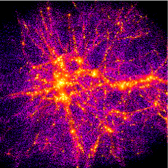
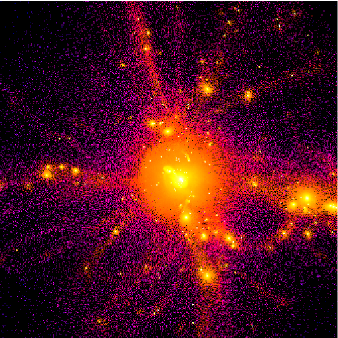
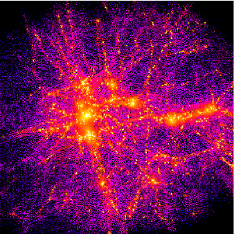
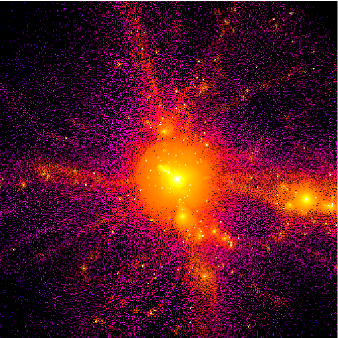
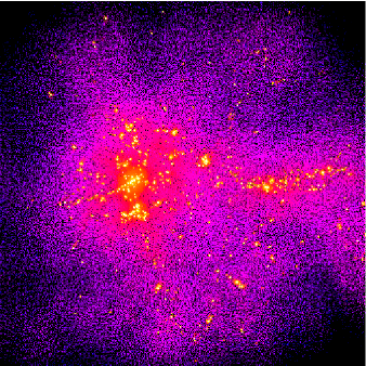
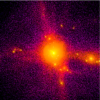
Figure 4: The maps of the gas density for simulations of a Virgo–like cluster at $z=2$ and $z=0$ (left and right panels, respectively), including cooling, star formation and different forms of non–gravitational heating. Upper panels are for a run which includes galactic winds with a velocity of about 340$\,{\rm km\,s^{-1}}$, the central panels is for galactic winds with velocity of about $830\,{\rm km\,s^{-1}}$ and the bottom panels is for galactic winds as in the top panels, but also adding a pre–heating with an entropy threshold of 100 keV cm² at $z=3$. At $z=0$ the size of the box is of $11.7\,h^{-1}{\rm Mpc}$, while at $z=2$ is corresponds to $17.5\,h^{-1}{\rm Mpc}$ comoving (from Borgani et al. 2005).

3 Scaling relations

So far, we have qualitatively discussed how simple models of pre–heating and radiative cooling can reproduce the observed violation of self–similarity in the X–ray properties of galaxy clusters. In this and in the following sections we will focus the discussion on a more detailed comparison between simulation results and observational data, and on the implications of this comparison on our current understanding of the feedback mechanisms which regulate star formation and the evolution of the galaxy population. As a starting point for the comparison between observed and simulated X–ray cluster properties, we describe how observable quantities are computed from hydrodynamical simulations and how they compare to the analogous quantities derived from observational data.

As for the X–ray luminosity, it is computed by summing the contributions to the emissivity, $\epsilon_{i}$, carried by all the gas elements (particles in a SPH run and cells in an Eulerian grid–based run), $L_{X}=\sum_{i}\epsilon_{i}$, where the sum extends over all the gas elements within the region where $L_{X}$ is computed. The contribution from the $i$-th gas element is usually written as

$$\epsilon_{i}\,=\,n_{{\rm e},i}n_{{\rm H},i}\Lambda(T_{i},Z_{i}){\rm d}V_{i}\,,$$ (8)

where $n_{{\rm e},i}$ and $n_{{\rm H},i}$ are the number densities of electrons and of hydrogen atoms, respectively, associated to the $i$-th gas element of given density $\rho_{i}$, temperature $T_{i}$ and metallicity $Z_{i}$. Furthermore, $\Lambda(T,Z)$ is the temperature– and metallicity–dependent cooling function (e.g., Sutherland & Dopita 1993) computed within a given energy band, while ${\rm d}V_{i}=m_{i}/\rho_{i}$ is the volume of the $i$-th gas element, having mass $m_{i}$.

As for the temperature, different proxies to its X–ray observational definition have been proposed in the literature, which differ from each other in the expression for the weight assigned to each gas element. In general, the ICM temperature can be written as

$$T\,=\,{\sum\limits_{i}w_{i}T_{i}\over\sum\limits_{i}w_{i}}\,,$$ (9)

where $T_{i}$ is the temperature of the $i$-gas element, which contributes with the weight $w_{i}$. The mass–weighted definition of temperature, $T_{\rm mw}$, is recovered for $w_{i}=m_{i}$ ($m_{i}$: mass of the $i$-th gas element), which also coincides with the electron temperature $T_{\rm e}$ for a fully ionised plasma. A more observation–oriented estimate of the ICM temperature is provided by the emission–weighted definition, $T_{\rm ew}$, which is obtained for $w_{i}=\epsilon_{i}$ (e.g., Evrard et al. 1996). The idea underlying this definition is that each gas element should contribute to the overall spectrum according to its emissivity.

Mazzotta et al. (2004) pointed out that the thermal complexity of the ICM is such that the overall spectrum is given by the superposition of several single–temperature spectra, each one associated to one thermal phase. In principle, the superposition of several single–temperature spectra cannot be described by a single–temperature spectrum. However, when fitting it to a single–temperature model in a typical finite energy band, where X–ray telescopes are sensitive, the cooler gas phases are relatively more important in providing the high–energy cut–off of the spectrum and, therefore, in determining the temperature resulting from the spectral fit. In order to account for this effect, Mazzotta et al. (2004) introduced a spectroscopic–like temperature, $T_{\rm sl}$, which is recovered from Eq. 9 by using the weight $w_{i}=\rho_{i}m_{i}T^{\alpha-3/2}$. By using $\alpha=0.75$, this expression for $T_{\rm sl}$ was shown to reproduce within few percent the temperature obtained from the spectroscopic fit, at least for clusters with temperature above 2–3 keV. More complex fitting expressions have been provided by Vikhlinin (2006), who generalised the spectroscopic–like temperature to the cases of lower temperature and arbitrary metallicity.

3.1 The luminosity–temperature relation

The $L_{X}$–$T$ relation represented the first observational evidence against the self–similar model. This relation has been shown by several independent analyses to have a slope, $L_{X}\propto T^{\alpha}$, with $\alpha\simeq 3$ for $T\gtrsim 2$ keV (e.g., White et al. 1997), with indications for a flattening to $\alpha\lesssim 2.5$ for the most massive systems (Allen & Fabian 1998). The scatter in this relation is largely contributed by the cool–core emission, so that it significantly decreases when excising the cores (Markevitch 1998) or removing cool–core systems (Arnaud & Evrard 1999). A change of behaviour is also observed at the scales of groups, $T\lesssim 2$ keV, which generally displays a very large scatter (Osmond & Ponman 2004).

Hydrodynamical simulations by Bialek et al. (2001) and by Borgani et al. (2002) demonstrated that simple pre–heating models, based on the injection of entropy at relatively high redshift, can reproduce the observed slope of the $L_{X}$–$T$ relation. Davé et al. (2002) showed that a similar result can also be achieved with simulations including cooling only, the price to be paid being a large overcooling. Muanwong et al. (2002) and Tornatore et al. (2003) demonstrated that combining cooling with pre–heating models can eventually decrease the total amount of stars to an acceptable level, while still providing a slope of the $L_{X}$–$T$ relation close to the observed one.

In Fig. 5 we show the comparison between observations and simulations in which the non–gravitational gas heating assumes the energy budget made available by the SN explosions, whose rate is computed from the simulated star formation rate. The left panel shows the results from the SPH GADGET simulations by Borgani et al. (2004). These simulations included the same model of kinetic feedback used in the simulations shown in the top panel of Fig. 4. This feedback model was shown by Springel & Hernquist (2003b) to be quite successful in producing a cosmic star formation history similar to the observed one. Quite apparently, these simulations provided a reasonable relation at the scale of clusters, $T\gtrsim 3$ keV, while failing to produce slope and scatter at the scale of groups.

The right panel show the results by Kay et al. (2007), which these authors plotted only for systems with $T>2$ keV. Kay et al. also used SPH simulations based on the GADGET code, but with a different feedback scheme. In this scheme, energy made available by SN explosions is assigned in a “targeted” way to suitably chosen gas particles, which surround the star–forming regions, so that their entropy is raised in such a way to prevent them from cooling. Therefore, while the amount of energy is self–consistently computed from star formation, the way in which it is thermalised to the gas is suitably tuned. These simulations predict a too high normalisation of the $L_{X}$–$T$ relation. This result is interpreted by Kay et al. (2007) as due to the fact that their simulations produce too low temperatures for clusters of a given mass, as a consequence of the incorrect cool–core structure.

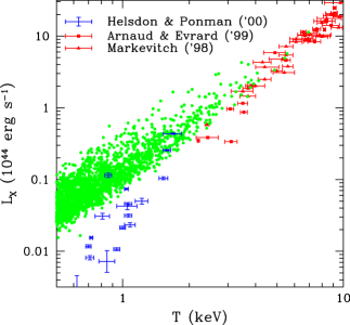
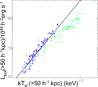
Figure 5: Left panel: The relation between bolometric X–ray luminosity and emission–weighted temperature for simulations by Borgani et al. (2004), including cooling, star formation and feedback in the form of galactic winds (green circles), compared with observational data for clusters (Arnaud & Evrard 1999; Markevitch 1998) and groups (Helsdon & Ponman 2000). Right panel: the relation between X–ray luminosity, estimated outside the core regions, and the spectroscopic–like temperature, for simulations which include cooling, star formation and a form of “targeted” feedback (from Kay et al. 2007). Observational data for clusters are the same as in the left panel.

Besides the slope of the local $L_{X}$–$T$ relation, also its evolution carries information about the thermodynamical history of the ICM. Thanks to the increasing statistics of distant clusters observed in the last years with Chandra and XMM–Newton, a number of authors analysed this evolution out to the highest redshifts, $z\simeq 1.3$, where clusters have been detected so far. These analyses generally indicate that the amplitude of the $L_{X}$–$T$ relation has a positive evolution out to $z\simeq 0.5$–0.6 (e.g. Arnaud et al. 2002; Lumb et al. 2004; Kotov & Vikhlinin 2005), with hints for a possible inversion of this trend at higher redshift (e.g. Ettori et al. 2004b; Maughan et al. 2006; Branchesi et al. 2007). In the attempt of interpreting these results, Voit (2005) showed that radiative cooling, combined with a modest amount of pre–heating with extra entropy, predicts an evolution of the $L_{X}$–$T$ relation slower than that of the self–similar model, also with an inversion of the trend at high redshift. Although in qualitative agreement with observations, these models have however difficulties in following the observed positive evolution at $z\lesssim 0.5$ (e.g., see Fig. 14 by Maughan et al. 2006).

As for the comparison with numerical predictions, Ettori et al. (2004a) analysed the evolution of the $L_{X}$–$T$ relation from the radiative simulation by Borgani et al. (2004), which includes the effect of SN feedback in the form of galactic winds. As a result, they found that the normalisation of this relation for the simulated clusters at high redshift is higher than for real clusters (see left panel of Fig. 6). Muanwong et al. (2006) analysed three sets of simulated clusters, based on radiative cooling only, on gas pre–heating at high redshift and on the same “targeted” SN feedback model used by Kay et al. (2007). As shown in the right panel of Fig. 6, they found that these three models predicts rather different evolutions of the $L_{X}$–$T$ relation, thus confirming it to be a sensitive test for the thermodynamical history of the ICM. However, so far none of the numerical models proposed is able to account for the observational indication for an inversion of the $L_{X}$–$T$ evolution at $z\simeq 0.5$. This represents still an open issue, whose implications for a realistic modelling of the ICM physics are still to be understood.

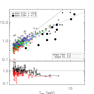
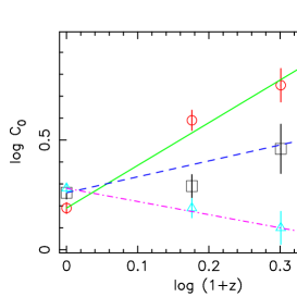
Figure 6: Left panel: A comparison of the evolution of the $L_{X}$–$T$ relation for the simulated clusters by Borgani et al. (2004) and the Chandra data analysed by Ettori et al. (2004b) (from Ettori et al. 2004a). The “plus” symbols are the relation at $z=0$, with the dotted and the dashed lines providing the best–fit relations when the slope is kept fixed at 2 and is left free, respectively. The squares, the triangles and the crosses show the simulation results at $z=0.5$, 0.7 and 1, respectively. The small and the big dots show the observational data at $0.5<z<0.8$ and at $z>0.8$, respectively. The lower panel shows the ratio between the measured luminosities at $z=0$ (“plus” symbols) and at $z=1$ (crosses) and the corresponding best–fitting power laws. Right panel: normalisation of the $L_{X}$–$T$ relation as a function of redshift, for the simulated clusters by Muanwong et al. (2006) in the radiative run with no feedback (solid line), in a run including an impulsive pre–heating at $z=4.5$ (dashed line), and in a run including a form of “targeted” feedback (dot–dashed line).

3.2 The mass–temperature relation

The relation between total collapsed mass and temperature has received much consideration both from the observational and the theoretical side, in view of its application for the use of galaxy clusters as tools to measure cosmological parameters (e.g., Voit 2005; Borgani 2006). The relation between ICM temperature and total mass should be primarily dictated by the condition of hydrostatic equilibrium. For this reason, the expectation is that this relation should have a rather small scatter and be insensitive to the details of the heating/cooling processes. For a spherically symmetric system, the condition of hydrostatic equilibrium translates into the mass estimator (e.g. Sarazin 1988)

$$M(<r)\,=\,-{r{\rm k}_{\rm B}T(r)\over G\mu m_{\rm p}}\left[{{\rm d}\,\ln\rho_{\rm gas}(r)\over{\rm d}\,\ln r}+{{\rm d}\,\ln T(r)\over{\rm d}\,\ln r}\right]\,.$$ (10)

Here $M(<r)$ is the total mass within the cluster-centric distance $r$, while $T(r)$ is the temperature measured at $r$. As shown in the previous section, the processes of heating/cooling are expected to modify the gas thermodynamics only in the central cluster regions, while the bulk of the ICM is dominated by gravitational processes. This implies that, in principle, the total mass estimate from Eq. 10 should be rather stable. However, since the $X$–ray spectroscopic temperature is sensitive to the thermal complexity of the ICM in the central regions (e.g., Mazzotta et al. 2004), a change of temperature and density profile in these regions may translate into a sizable effect in the mass–temperature relation provided by Eq. 10.

Eq. 10 has been often applied in the literature by modelling the gas density profile with a $\beta$–model (Cavaliere & Fusco-Femiano 1976),

$$\rho_{\rm gas}(r)\,=\,{\rho_{0}\over\left[1+(r/r_{\rm c})^{2}\right]^{3\beta/2}}\,,$$ (11)

where $r_{\rm c}$ is the core radius, and assuming either isothermal gas or a polytropic gas, $\rho_{\rm gas}\propto T^{\gamma-1}$, to account for the presence of temperature gradients. In this case, Eq. 10 can be recast in the form

$$M(<r)\,\simeq\,1.1\times 10^{14}\beta\gamma\,{T(r)\over{\rm keV}}\,{r\over\,h^{-1}{\rm Mpc}}\,{(r/r_{\rm c})^{2}\over 1+(r/r_{\rm c})^{2}}\,.$$ (12)

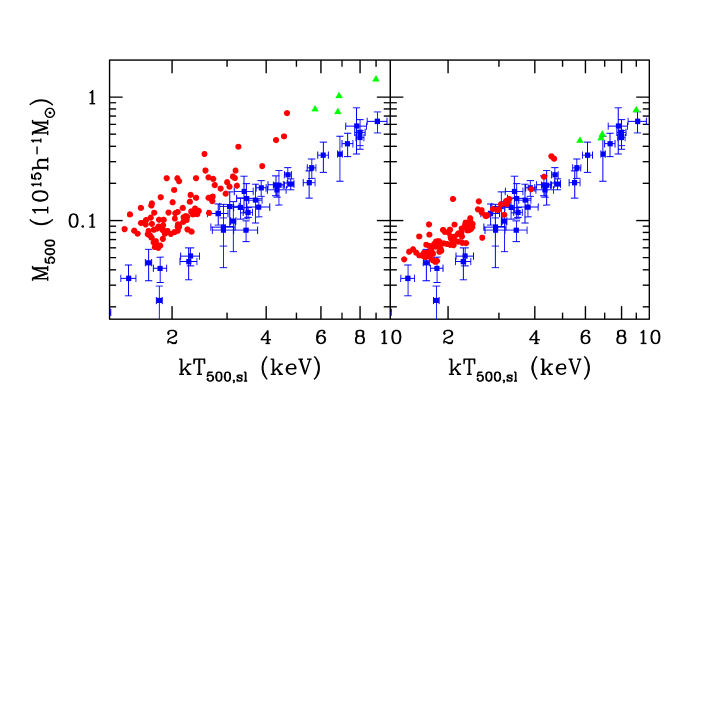
Figure 7: The relation between mass and spectroscopic–like temperature within $r_{500}$. Red circles and green triangles are for simulations, which include cooling, star formation and feedback from galactic winds, while squares with error bars are the observational data by Finoguenov et al. (2001). Left panel: $M_{500}$ exactly computed by summing the mass of all the particles within $r_{500}$. Right panel: $M_{500}$ estimated as in the observational data, by using the equation of hydrostatic equilibrium for a polytropic $\beta$–model. From Rasia et al. (2005).

Based on the analysis of non–radiative cluster simulations, Schindler (1996) and Evrard et al. (1996) argued that the X–ray temperature provides a rather precise determination of the cluster mass, with an intrinsic scatter of only about 15 per cent at $r_{500}$. Finoguenov et al. (2001) applied Eq. 12 to ROSAT imaging and ASCA spectroscopic data (see also Nevalainen et al. 2000). They found that the resulting $M$–$T$ relation has a normalisation about 40 per cent lower than that from the simulations by Evrard et al. (1996). Although introducing the effect of cooling, star formation and SN feedback provides a 20 per cent lower normalisation, this was not yet enough to recover agreement with observations. Independent analyses (Muanwong et al. 2002; Borgani et al. 2004) showed that applying to simulated clusters Eq. 12, which is used to estimate masses of real clusters, leads to a mass underestimate of about 20 per cent. This bias in the mass estimate is enough to bring the simulated and the observed $M$–$T$ relations into reasonable agreement. These analyses were still based on the emission–weighted temperature in the simulation analysis.

Rasia et al. (2005) showed that using the spectroscopic–like definition, $T_{\rm sl}$, leads to a mass underestimate of up to $\sim 30$ per cent with respect to the true cluster mass. This result is shown in Fig. 7. The left panel reports the relation between $T_{\rm sl}$ for simulated clusters and the true total cluster mass, also compared with the observed $M$–$T$ relation by Finoguenov et al. (2001). Quite apparently, the relation from simulations lies well above the observational one. However, this difference is much reduced in the right panel, where the masses of the simulated clusters are computed by applying Eq. 12. The reason for this difference between “true” and “recovered” masses is partly due to the violation of hydrostatic equilibrium, associated to subsonic gas bulk motions (e.g., Rasia et al. 2004; Nagai et al. 2007b) and partly to the poor fit provided by the $\beta$–model (e.g., Ascasibar et al. 2003) when extended to large radii. It is also interesting to note that the mass estimator of Eq. 12 also under-predicts the intrinsic scatter of the $M$–$T$ relation from the simulations. This is due to the fact that the equation of hydrostatic equilibrium imposes a strong correlation between ICM temperature and total mass. Any scatter is then associated to a cluster-by-cluster variation of the parameters $\beta$ and $\gamma$, which may not be fully representative of the diversity of the ICM structure among different objects.

Using XMM–Newton and Chandra data, different authors (e.g., Arnaud et al. 2005; Vikhlinin et al. 2005) applied the equation of hydrostatic equilibrium by avoiding the assumption of a simple beta–model for the gas density profile. As a result, the observed and the simulated $M$–$T$ relations turned out to agree with each other, especially when simulated clusters are analysed in the same way as real clusters (e.g., Rasia et al. 2006; Nagai et al. 2007b). The left panel of Fig. 8 shows the comparison between the observational results by Arnaud et al. (2005) and simulations. Here the discrepancy with respect to the non–radiative runs by Evrard et al. (1996) is alleviated when including the effect of star formation and SN feedback (Borgani et al. 2004). In a similar way, the right panel shows the comparison between the observed $M$–$T$ relation by Vikhlinin et al. (2005) and the simulations by Nagai et al. (2007a) who computed cluster masses by using the same method applied to the Chandra data. This plot further demonstrates the good level of agreement between simulated and observed $M$–$T$ relation, once the 15–20 percent violation of hydrostatic equilibrium is taken into account.

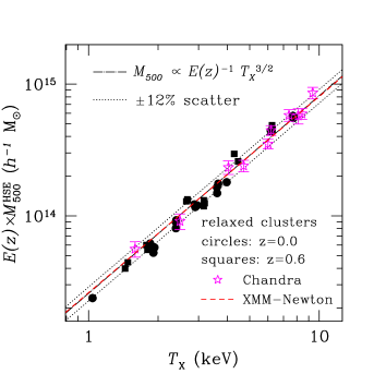
Figure 8: Left panel: the observed mass–temperature relation at $r_{500}$ for nearby clusters observed with XMM–Newton, compared with $M$–$T$ relations from simulations (from Arnaud et al. 2005). The solid line is the best fit to observations, while the dotted line is the best fit only to a subsample of hot clusters. The short-dashed line is the relation from the non–radiative simulations by Evrard et al. (1996), while the long–dashed line is the relation from the radiative simulations by Borgani et al. (2004). Right panel: the $M$–$T$ relation at $r_{500}$ from the radiative simulations by Nagai et al. (2007a); circles: $z=0$; squares: $z=0.6$, which include cooling, star–formation and an inefficient form of SN feedback, compared to Chandra observations for a set of nearby relaxed clusters by Vikhlinin et al. (2005); stars with error bars. Masses of simulated clusters have been computed by using the same estimator, based on the hydrostatic equilibrium, applied to the Chandra data. Masses of both simulated and observed clusters have been rescaled with redshift according to the evolution predicted by the self–similar model.

3.3 The mass–”pressure” relation

To first approximation, the ICM can be represented by a smooth gas distribution in pressure equilibrium within the cluster potential well. Therefore, the expectation is that gas pressure should be the quantity that is more directly correlated to the total collapsed mass. For this reason, any pressure–related observational quantity should provide a robust minimum–scatter proxy to the cluster mass. One such observable is the Comptonisation parameter, measured through the Sunyaev-Zeldovich effect (SZE; e.g., Carlstrom et al. 2002, for a review), which is proportional to the ICM pressure integrated along the line of sight. Observations of the SZ effect are now reaching a high enough quality for extended sets of clusters, to allow correlating the SZ signal with X–ray observable quantities. For instance, Bonamente et al. (2007) analysed a set of 38 massive clusters in the redshift range $0.14\leq z\leq 0.89$, for which both SZE imaging from the OVRO/BIMA interferometric array and Chandra X–ray observations are available. As a result, they found that the slope and the evolution of the scalings of the Comptonisation parameter with gas mass, total mass and X–ray temperature are all in agreement with the prediction of the self–similar model.

In an attempt to provide an X–ray observable related to the pressure, Kravtsov et al. (2006) introduced the quantity $Y_{X}=M_{\rm gas}T$, defined by the product of the total gas mass times the temperature, both measured within a given aperture. With this definition, $Y_{X}$ represents the X–ray counterpart of the Compton-$y$ parameter, measured from the SZ effect. By computing this quantity for a set of simulated clusters, Kravtsov et al. (2006) showed that $Y_{X}$ has a very tight correlation with the cluster mass, with a remarkably small scatter of only 8 per cent. The application to Chandra observations of a set of nearby relaxed clusters also shows that this relation has a comparably small scatter. Again, once masses of simulated and observed clusters are computed by applying the same hydrostatic estimator, the normalisation of the $Y_{X}$–$M$ relation from models and data closely agree with each other (Nagai et al. 2007a; see left panel of Fig. 9). Since mass is determined in this case from temperature, $Y_{X}$ and $M$ are not independent quantities and, therefore, the scatter in their scaling relation may be underestimated.

Maughan (2007) computed $Y_{X}$ for an extended set of clusters extracted from the Chandra archive, in the redshift range $0.1<z<1.3$. The results of his analysis, shown in the right panel of Fig. 9, indicate that $Y_{X}$ is also tightly correlated with the X–ray luminosity through a relation which evolves in a self–similar way. Again, since the gas mass is obtained from the X–ray surface brightness, $Y_{X}$ and $L_{X}$ are not independent quantities, thus possibly leading to an underestimate of the intrinsic scatter in their scaling relation.

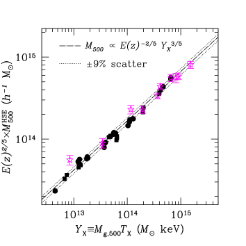
Figure 9: Left panel: the relation between $Y_{X}=M_{\rm gas}T_{X}$ and $M_{500}$. Points with error bars are for Chandra observational data (from Nagai et al. 2007a). Masses of simulated clusters have been computed by using the same estimator, based on the hydrostatic equilibrium, applied to the Chandra data. Masses of both simulated and observed clusters have been rescaled with redshift according to the evolution predicted by the self–similar model. Right panel: the relation between $Y_{X}$ and the $X$–ray luminosity, both estimated within $r_{500}$, for a set of clusters at $0.1<z<1.3$ extracted from the Chandra archive (from Maughan 2007). Luminosities have been rescaled according to the redshift dependence expected from self–similar evolution.

3.4 The gas mass fraction

The measurement of the baryon mass fraction in nearby galaxy clusters has been recognised for several years to be a powerful method to measure the cosmological density parameter (e.g., White et al. 1993; Mohr et al. 1999), while its redshift evolution provides constraints on the dark energy content of the Universe (e.g., Allen et al. 2002; Ettori et al. 2003, and references therein). Since diffuse gas dominates the baryon budget of clusters, a precise measurement of the ICM total mass represents a fundamental step in the application of this cosmological test. While this method relies on the basic assumption that all clusters contain baryons in a cosmic proportion, a number of observational evidences show that the gas mass fraction is smaller in lower temperature systems (Lin et al. 2003; Sanderson et al. 2003). This fact forces one to restrict the application to the most massive and relaxed systems. In addition, since X–ray measurements of the gas mass fraction are generally available only out to a fraction of the cluster virial radius, the question then arises as to whether the gas fraction in these regions is representative of the cosmic value. Indeed, observational evidence has been found for an increase of the gas mass fraction with radius (e.g., Castillo-Morales & Schindler 2003).

In this respect, hydrodynamical simulations offer a way to check how the gas mass is distributed within individual clusters and as a function of the cluster mass, thus possibly providing a correction for such biases. Indeed, Allen et al. (2004) resorted to the set of SPH clusters simulated by Eke et al. (1998) to calibrate the correction factor that one needs to apply to extrapolate the baryon fraction computed at $r_{2500}$, which is the typical radius at which it is measured, to the cosmic value. However, since this set of simulations does not include the effects of cooling, star formation and feedback heating, it is not clear whether they provide a reliable description of the gas distribution within real clusters.

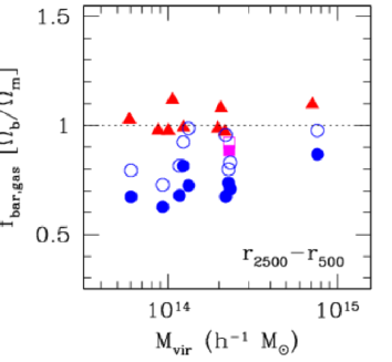
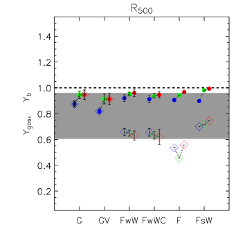
Figure 10: Left panel: the gas fraction (filled circles) and the baryon fraction (open circles) for cluster simulations which include cooling and star formation. Squares indicate runs where cooling is switched off at $z<2$, while triangles are for non–radiative simulations (from Kravtsov et al. 2005). Right panel: the gas fraction (diamonds) and the baryon fraction (circles) within $r_{500}$ for SPH simulations of clusters, which include different gas physics. G: gravitational heating only; GV: G with a scheme for reduced SPH gas viscosity; FwW: radiative runs with feedback and weak galactic winds; FwWC: like FwW with also thermal conduction, with an efficiency of one–third of the Spitzer value; F: radiative runs with no winds; FsW: radiative runs with strong winds. Blue, green and red symbols refer to redshifts $z=0$, 0.7 and 1 (from Ettori et al. 2006). The shaded area indicates the range of values of the observed gas fraction (Ettori & Fabian 1999).

Kravtsov et al. (2005) used high resolution simulations, based on an Eulerian code, for a set of clusters using both non–radiative and radiative physics. They found that including cooling and star formation has a substantial effect on the total baryon fraction in the central cluster regions, where it is even larger than the cosmic value. As shown in the left panel of Fig. 10, at the virial radius the effect is actually inverted, with the baryon fraction of radiative runs lying below that of the non–radiative runs. In addition, they also compared results obtained from Eulerian and SPH codes and found small, but systematic, differences between the resulting baryon fractions.

Ettori et al. (2006) performed a similar test, based on SPH simulations, but focusing on the effect of changing in a number of ways the description of the relevant physical processes, such as gas viscosity, feedback strength and thermal conduction. The results of their analysis, which is shown in the right panel of Fig. 10, demonstrated that the baryon fraction is generally stable but only at rather large radii, $\gtrsim r_{500}$. They also showed that changing the description of the relevant ICM physical processes changes the extrapolation of the baryon fraction from the central regions, relevant for X–ray measurements, while also slightly affecting the redshift evolution.

On the one hand, these results show that simulations can be used as calibration instruments for cosmological applications of galaxy clusters. On the other hand, they also demonstrate that for this calibration to reach the precision required to constrain the dark energy content of the Universe, one needs to include in simulations the relevant physical processes which determine the ICM observational properties.

4 Profiles of X–ray observables

4.1 The temperature profiles

Already ASCA observations, despite their modest spatial resolution, have established that most of the clusters show significant departures from isothermality, with negative temperature gradients characterised by a remarkable degree of similarity, out to the largest radii sampled (e.g., Markevitch et al. 1998). Besides confirming the presence of these gradients, Beppo–SAX observations (e.g. De Grandi & Molendi 2002) showed that they do not extend down to the innermost cluster central regions, where instead an isothermal regime is observed, possibly followed by a decline of the temperature towards the centre, at least for relaxed clusters. The much improved sensitivity of the Chandra satellite provides now a more detailed picture of the central temperature profiles (e.g., Vikhlinin et al. 2005; Baldi et al. 2007). At the same time, a number of analyses of XMM–Newton observations now consistently show the presence of a negative gradient at radii $\gtrsim 0.1r_{200}$ (e.g., Piffaretti et al. 2005; Pratt et al. 2007, and references therein). Relaxed clusters are generally shown to have a smoothly declining profile toward the centre, reaching values which are about half of the overall virial cluster temperature in the innermost sampled regions, with non–relaxed clusters having, instead, a larger variety of temperature profiles. The emerging picture suggests that gas cooling is responsible for the decline of the temperature in the central regions, while some mechanism of energy feedback should be responsible for preventing overcooling, thereby suppressing the mass deposition rate and the resulting star formation.

As for hydrodynamical simulations, they have shown to be generally rather successful in reproducing the declining temperature profiles outside the core regions (e.g., Loken et al. 2002; Roncarelli et al. 2006), where gas cooling is relatively unimportant. On the other hand, as we have already discussed in Sect. 2.2, including gas cooling has the effect of steepening the $T$– profiles in the core regions, in clear disagreement with observations. The problem of the central temperature profiles in radiative simulations has been consistently found by several independent analyses (e.g. Valdarnini 2003; Borgani et al. 2004; Nagai et al. 2007a) and is interpreted as due to the difficulty that currently implemented feedback schemes have in balancing the cooling runaway.

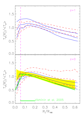
Figure 11: Left panel: the temperature profiles in AMR simulations of clusters (thick curves) and in real clusters (thin curves). The simulation results are the average over 16 numerical clusters. The solid line is for runs with cooling and star formation, while the dashed line is for non–radiative simulations. The observational curves are for clusters with different temperatures (from Nagai et al. 2007a). Right panel: Temperature profiles at $z=1$ (top) and at $z=0$ (bottom) from a set of SPH simulated clusters including cooling, star–formation and a “targeted” scheme of SN feedback (from Kay et al. 2007). Median and 10/90 percentiles are shown. Solid and dashed lines are for irregular and regular clusters, respectively. The vertical dashed line indicates the smallest scale which is numerically resolved. In the bottom panel, the heavy green line shows the profile from Chandra observations of cool core clusters (Vikhlinin et al. 2005), while the yellow shaded area is for a XMM–Newton sample of nearby clusters (Pratt et al. 2007).

As an example, we show in the left panel of Fig. 11 the comparison between simulated and observed temperature profiles, recently presented by Nagai et al. (2007a), which is based on a set of clusters simulated with an Adaptive Mesh Refinement (AMR) code. This plot clearly shows that the central profiles of simulated clusters are far steeper than the observed ones, by an amount which increases when cooling and star formation are turned on. Although this result is in qualitative agreement with other results based on SPH codes, an eye-ball comparison with the left panel of Fig. 3 shows a significant difference of the profiles in the central regions for the non–radiative runs. Indeed, while SPH simulations generally show a flattening at $r\lesssim 0.1r_{\rm vir}$, Eulerian simulations are instead characterised by continuously rising profiles. While this difference is reduced when cooling is turned on, it clearly calls for the need of performing detailed comparisons between different simulation codes, in the spirit of the Santa Barbara Cluster Comparison Project (e.g. Frenk et al. 1999), and to understand in detail the reason for these differences.

As discussed above, the steep temperature profiles predicted in the central regions witness the presence of overcooling. Viceversa, the fact that a feedback mechanism is able to produce the correct temperature profiles does not guarantee in itself that overcooling is prevented. Indeed, Kay et al. (2007) found that their “targeted” scheme of SN feedback produces temperature profiles which are in reasonable agreement with observations (see the right panel of Fig. 11). However, even with this efficient feedback scheme, the resulting stellar fraction within clusters was still found to be too high, $\gtrsim 25$ per cent, thus indicating the presence of a substantial overcooling in their simulations.

Clearly, resolving the discrepancy between observed and simulated central temperature profiles requires that simulations are able to produce the correct thermal structure of the observed “cool cores”. This means that a suitable feedback should compensate the radiative losses of the gas at the cluster centre, while keeping it at about $\sim 1/3$ of the virial temperature. A number of analyses converge to indicate that AGN should represent the natural solution to this problem. Considerable efforts have been spent to investigate how cooling can be self–consistently regulated by feedback from a central AGN in static cluster potentials (e.g., Churazov et al. 2001; Omma et al. 2004; Brighenti & Mathews 2006; Sternberg et al. 2007, and reference therein), while only quite recently these studies have been extended to clusters forming in a cosmological context (e.g., Heinz et al. 2006; Sijacki et al. 2007). Although the results of these analyses are quite promising, we still lack for a detailed comparison between observational data and an extended set of cosmological simulations of clusters, convincingly showing that AGN feedback is able to provide the correct ICM thermal structure for objects spanning a wide range of masses, from poor groups to rich massive clusters.

4.2 The entropy profiles

As already mentioned in Sect. 2, a convenient way of characterising the thermodynamical properties of the ICM is through the entropy, which, in X–ray cluster studies, is usually defined as $S=T/n_{\mathrm{e}}^{2/3}$ (see the review by Voit 2005, for a detailed discussion about the role of entropy in cluster studies). Since the current numerical description of the heating/cooling interplay in the central cluster regions is unable to reproduce the observed temperature structure, there is no surprise that simulations have difficulties also in accounting for the observed entropy structure. However, while the ICM thermodynamics is sensitive to complex physical processes in the core regions, one expects simulations to fare much better in the outer regions, say at $r>0.2\,r_{200}$, where the gas dynamics should be dominated by gravitational processes. This expectation is also supported by the agreement between the observed and the simulated slope of the temperature profiles outside cluster cores.

If gravity were the only process at work, then the prediction of the self–similar model is that $S\propto T$. Therefore, by plotting profiles of the reduced entropy, $S/T$, one expects them to fall on the top of each other for clusters of different temperatures. However, observations revealed that this is not the case. Indications from ASCA data (Ponman et al. 2003) showed that entropy profiles of poor clusters and groups have an amplitude which is higher than that expected for rich clusters from the above scaling argument. This result has been subsequently confirmed by the XMM–Newton data analysed by Pratt & Arnaud (2005) and by Piffaretti et al. (2005). Quite remarkably, a relatively higher entropy for groups is found not only in the central regions, where it can arise as a consequence of the heating/cooling processes, but extends to all radii sampled by X–ray observations, out to $\lesssim 0.5r_{500}$. These analyses consistently indicate that $S\propto T^{\alpha}$, with $\alpha\simeq 0.65$, instead of $\alpha=1$ as expected from self–similar scaling.

Ponman et al. (2003) and Voit et al. (2003) interpreted this entropy excess in poor clusters and groups as the effect of entropy amplification generated by shocks from smoothed gas accretion. The underlying idea is the following. In the hierarchical scenario for structure formation, a galaxy group is expected to accrete from relatively smaller filaments and merging sub–groups than a rich cluster does. Suppose now to heat the gas with a fixed amount of specific energy (or entropy). Such a diffuse heating will be more effective to smooth the accretion pattern of a group than that of a rich cluster, just as a consequence of the lower virial temperature of the structures falling into the former object. In this case, accretion shocks take place at a lower density and, therefore, are more efficient in generating entropy. While predictions from the semi–analytical approach by Voit et al. (2003) are in reasonable agreement with observational results, one may wonder whether these predictions are confirmed by full hydrodynamical simulations.

To tackle this problem, Borgani et al. (2005) performed a series of SPH hydrodynamical simulations of four galaxy clusters and groups, with temperature in the range 0.5–3 keV, using both non–radiative and radiative runs, also exploring a variety of heating recipes. As a result, they found that galactic ejecta powered by an even extremely efficient SN feedback are not able to generate the observed level of entropy amplification. This result is shown in the left panel of Fig. 12 where the profiles of reduced entropy are plotted for the simulated structures in the case of moderate (upper panel) and very strong (bottom panel) galactic outflows. Borgani et al. also showed that only adding an entropy floor at $z=3$ provides an efficient smoothing of the gas accretion pattern and, therefore, a substantial degree of entropy amplifications (see Fig. 4). Although this diffuse pre–heating provides an adequate entropy amplification at large radii, the price to pay is that the entropy level is substantially increased in the central regions. This is at variance with high–resolution Chandra measurements of low entropy gas in the innermost cluster regions, where it reaches values as low as $\sim 10$ keV cm² (Donahue et al. 2006).

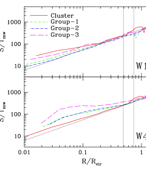
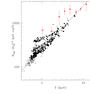
Figure 12: Left panel: the profile of reduced entropy, $S/T$, for a series of SPH GADGET runs of one cluster and three groups, including cooling, star formation and feedback from galactic winds. The top panel is for runs in which the winds have a velocity of about $360~{}\,{\rm km\,s^{-1}}$, while the bottom panel is for an extreme wind model with a velocity of $830~{}\,{\rm km\,s^{-1}}$ (from Borgani et al. 2005). The straight dotted line marks the slope $S\propto R^{0.95}$ which is the best–fitting to the observed entropy profiles (Pratt & Arnaud 2005; Piffaretti et al. 2005). Right panel: the relation between entropy computed at $r_{500}$ for clusters and groups identified in AMR ENZO cosmological simulations (from Younger & Bryan 2007), compared with the observational results by Ponman et al. (2003); symbols with error bars. Shown are four different cases of entropy injection at $z=10$: no pre-heating (open triangles), 78 keV cm² (filled circles), 155 keV cm² (stars), 311 keV cm² (filled triangles). The solid line is a power–law fit to the self–similar prediction from the simulations.

A similar analysis has also been performed by Younger & Bryan (2007), who used a set of AMR non–radiative cosmological simulations performed with the ENZO code (O’Shea et al. 2004), with gas entropy boosted at high redshift, $z=10$. In keeping with previous analyses, they found that pre–heated simulations are generally able to reproduce the observed luminosity–temperature and mass–temperature relations. However, differently from Borgani et al. (2005), even the most extreme pre–heating scheme does not provide an appreciable degree of entropy amplification. This result is shown in the right panel of Fig. 12. The deviations from self–similarity for the entropy computed at $r_{500}$ are always too small to reconcile the simulations with the observational data by Ponman et al. (2003). A possible reason for the different results with respect to the analysis by Borgani et al. is due to the higher redshift of pre–heating, $z=10$ instead of 3, used by Younger & Bryan. Furthermore, grid–based codes are known to produce entropy profiles that, in the central part of the halos, $r\lesssim 0.2r_{200}$, are flatter than those produced by SPH codes (e.g., Voit et al. 2005). Therefore, the question arises as to whether different numerical schemes of hydrodynamics react in different ways to pre–heating. It would be highly recommendable that future simulation comparison projects will include tests of how different codes behave in the presence of simple schemes of non-gravitational heating.

5 Summary

In this paper we reviewed the current status of the comparison between cosmological hydrodynamical simulations of the X–ray properties of the intra–cluster medium (ICM) and observations. We first presented the basic predictions of the self–similar model, based on the assumption that only gravitational processes drive the evolution of the ICM. We then showed how a number of observational facts are at variance with these predictions, with poor clusters and groups characterised by a relatively lower density and higher entropy of the gas. This calls for the need of introducing some extra physical processes, such as non–gravitational heating and radiative cooling, which are able to break the self–similarity between objects of different size. The results based on simulations, which include these effects, can be summarised as follows.
(1) The observed scaling relation between X–ray luminosity and temperature can be reproduced by simulations including cooling only, but at the expense of producing a too large fraction of cooled gas. Introducing ad–hoc schemes of entropy injection at high redshift (the so–called pre–heating) can eventually produce the correct $L_{X}$–$T$ relation. However, no simulations have been presented so far, in which a good agreement with observations is achieved by using a feedback scheme in which the energy release and thermalisation from SN or AGN is self–consistently computed by the simulated star formation or accretion onto a cosmologically evolving population of black holes.
(2) Simulations which include cooling, star formation and SN feedback, correctly reproduce the observed mass–temperature and “pressure”–temperature relations. Quite interestingly, this agreement is achieved once the masses of simulated clusters are estimated by applying the same mass estimators, based on the assumption of hydrostatic equilibrium, which are applied to the analysis of real clusters. The violation of hydrostatic equilibrium, related to the non–thermal pressure support from subsonic gas motions, would otherwise lead to a $\sim 20$ per cent overestimate of the normalisation of the above scaling relations for simulated clusters.
(3) Both non–radiative and radiative runs naturally predict the observed negative gradients of the temperature profiles outside the cluster core regions, $r\gtrsim 0.2r_{200}$. This suggests that the ICM thermal structure in these regions is indeed dominated by the action of gravitational processes, such as heating from shocks associated to supersonic gas accretion.
(4) Introducing cooling has the effect of steepening the temperature profiles in the innermost regions, as a consequence of the adiabatic compression of inflowing gas, caused by the lack of pressure support. Therefore, gas in the cores of simulated clusters generally lies in a high–temperature phase, which is very well separated from the cold ($\sim 10^{4}$ K) phase. This is at variance with the observed “cool core” structure of real clusters, which show instead the presence of a fair amount of gas, down to a limiting temperature of $\sim 1/3$ of the virial temperature, which formally has a rather short cooling time. The presence of this gas makes the observed temperature profiles of relaxed clusters to peak at $r\simeq 0.2r_{200}$, thereby decreasing by about a factor two in the innermost sampled regions. The discrepancy between the simulated and the observed “cool core” calls for the need of introducing in cluster simulations a suitable feedback mechanism which is able to compensate the radiative losses, keeps pressurised gas in the central regions, and suppresses the mass deposition rate.
(5) Simulations are generally rather successful in reproducing the observed slope of the entropy profiles outside the core regions, $S\propto r^{\alpha}$ with $\alpha\simeq 1$. This slope is also close to that predicted by models based on gravitational heating from spherical accretion, thus lending further support to the picture that gravity drives the evolution of the ICM outside the core regions. Quite intriguingly, however, the normalisation of the profiles out to the largest sampled radii, $\lesssim r_{500}$, is observed to have a milder temperature dependence than expected from the self–similar model, $S\propto T^{\alpha}$ with $\alpha\simeq 0.65$ instead of $\alpha\simeq 1$. This entropy excess in poor systems can be reproduced in simulations only by adding a diffuse pre–heating mechanism, which smoothes the pattern of gas accretion, thereby leading to an amplification of entropy generation from shocks in poorer systems. However, this mechanism is able to provide the correct explanation only for clusters with temperature $T\lesssim 3$ keV. Generating entropy amplification in hotter systems would require an exceedingly large amount of pre–heating, which would generate too shallow entropy profiles.

In general, the above results demonstrate the capability of cosmological hydrodynamical simulations to predict the correct thermodynamical properties of the ICM outside the central regions of galaxy clusters. On the other hand, even simulations based on an efficient SN feedback fail in preventing overcooling and providing the correct description of the thermodynamical ICM properties in the central regions. The “cool core” failure of simulations based on stellar feedback is also witnessed by the exceedingly massive and blue central galaxies that are generally produced (see also Borgani et al. 2008 - Chapter 18, this volume).

The fact that cool cores are observed for systems spanning at least two orders of magnitude in mass, from $\sim 10^{13}M_{\odot}$ to $\sim 10^{15}M_{\odot}$, suggests that only one self–regulated mechanism should be mainly responsible for this, rather than the combination of several mechanisms possibly acting over different time–scales. Although AGN are generally thought to naturally provide such a mechanism, a detailed comparison between observational data and an extended set of cluster simulations, including this kind of feedback is still lacking. Furthermore, understanding in detail the role of AGN in determining the ICM properties requires addressing in detail two major issues. Firstly, the accretion process onto the central black hole involves scales of the order of the parsec, while the X–ray observable effects involve scales of $\sim 10$–100 kpc. This requires understanding the cross–talk between two ranges of scales, which differ by at least four orders of magnitude. Secondly, the total energy budget available from AGN is orders of magnitude larger than that required to regulate cooling flows. Therefore, one needs ultimately to understand the channels for the thermalisation of the released energy and how this naturally takes place without resorting to any ad–hoc tuning. These problems definitely need to be addressed by simulations of the next generation, which will be aimed at understanding in detail the evolution of the cosmic baryons and the observational X–ray properties of galaxy clusters.