Phase-coherent timing of the accreting millisecond pulsar SAX J1748.9-2021

Abstract

We present a phase-coherent timing analysis of the intermittent accreting millisecond pulsar SAX J1748.9$-$2021. A new timing solution for the pulsar spin period and the Keplerian binary orbital parameters was achieved by phase connecting all episodes of intermittent pulsations visible during the 2001 outburst. We investigate the pulse profile shapes, their energy dependence and the possible influence of Type I X-ray bursts on the time of arrival and fractional amplitude of the pulsations. We find that the timing solution of SAX J1748.9$-$2021 shows an erratic behavior when selecting different subsets of data, that is related to substantial timing noise in the timing post-fit residuals. The pulse profiles are very sinusoidal and their fractional amplitude increases linearly with energy and no second harmonic is detected. The reason why this pulsar is intermittent is still unknown but we can rule out a one-to-one correspondence between Type I X-ray bursts and the appearance of the pulsations.

1 Introduction

Recently it has been shown (Kaaret et al. 2006, Galloway et al. 2007, Casella et al. 2007, Gavriil et al. 2007, Altamirano et al. 2007) that intermittent pulsations can be observed during the transient outbursts of some accreting millisecond pulsars (AMPs). It was emphasized (Casella et al. 2007, Gavriil et al. 2007, Altamirano et al. 2007) that a new class of pulsators is emerging with a variety of phenomenology i.e., pulsations lasting only for the first two months of the outburst (HETE J1900.1-2455, Kaaret et al. 2006, Galloway et al. 2007), switching on and off throughout the observations (SAX J1748.9-2021, Altamirano et al. 2007, and HETE J1900.1-2455 Galloway et al. 2007), or even appearing for only  150 s over 1.3 Ms of observations (Aql X-1, Casella et al. 2007). This is different from the behavior of other known AMPs, where the pulsations persist throughout the outburst until they drop below the sensitivity level of the instrumentation.

Galloway et al. (2007) and Altamirano et al. (2007) pointed out the clear, albeit non-trivial, connection between the appearance of pulsations in HETE J1900.1-2455 and SAX J1748.9-2021 and the occurrence of thermonuclear bursts (Type I X-ray bursts). Galloway et al. (2007) demonstrated that increases of pulse amplitude in HETE J1900.0$-$2455 sometimes but not always follow the occurrence of Type I bursts nor do all bursts trigger an increase in pulse amplitude. Altamirano et al. (2007) showed that in SAX J1748.9$-$2021 the pulsations can re-appear after an absence of pulsations of a few orbital periods or even a few hundred seconds. All the pulsing episodes occur close in time to the detection of a Type I X-ray burst, but again not all the Type I bursts are followed by pulsations so it is unclear if the pulsations are indeed triggered by Type I X-ray bursts.
The pulse energy dependence and the spectral state in which pulsations are detected also differ between these objects. As shown by Cui et al. (1998), Galloway et al. (2005), Gierliński & Poutanen (2005) and Galloway et al. (2007), the fractional amplitude of the pulsations in AMPs monotonically decreases with increasing energies between 2 and $\approx 20$keV. However in IGR J00291+5934, Falanga et al. (2005) found a slight decrease in the pulse amplitude between 5 and 8 keV followed by an increase up to energies of 100 keV. For the single pulse episode of Aql X-1 the pulsation amplitude increased with energy between 2 and $\approx 20$keV (Casella et al. 2007). Interestingly in Aql X-1 the pulsations appeared during the soft state, contrary to all the other known AMPs which pulsate solely in their hard state (although many of these objects have not been observed in a soft state). Therefore it is interesting to investigate these issues for SAX J1748.9$-$2021 as well.
In order to study these various aspects of SAX J1748.9$-$2021 an improved timing solution is necessary. The spin frequency of the neutron star and the orbital parameters of SAX J1748.9$-$2021 were measured by Altamirano et al. (2007) using a frequency-domain technique that measures the Doppler shift of the pulsar spin period due to the orbital motion of the neutron star around the center of mass of the binary. The source was found to be spinning at a frequency of 442.361 Hz in a binary with an orbit of  8.7 hrs and a donor companion mass of $\sim 0.1-1M_{\odot}$. However, the timing solution obtained with this technique was not sufficiently precise to phase connect between epochs of visible pulsations. The intermittency of the pulsations creates many gaps between measurable pulse arrival times, complicating the use of standard techniques to phase connect the times of arrival (TOAs). The current work presents a follow-up study to the discovery paper of intermittent pulsations in SAX J1748.9$-$2021 (Altamirano et al. 2007) and provides for the first time a timing solution obtained by phase connecting the pulsations observed during the 2001 outburst. In §2 we present the observations and in §3 we explain the technique employed to phase connect the pulsations. In §4 we show our results and in §5 we discuss them. In §6 we outline our conclusions.

2 X-ray observations and data reduction

We reduced all the pointed observations from the RXTE Proportional Counter Array (PCA, Jahoda et al. 2006) that cover the 1998, 2001 and 2005 outbursts of SAX J1748.9$-$2021. The PCA instrument provides an array of five proportional counter units (PCUs) with a collecting area of 1200 $\rm\,cm^{2}$ per unit operating in the 2-60 keV range and a field of view of $\approx 1^{\circ}$. The number of active PCUs during the observations varied between two and five. We used all the data available in the Event mode with a time resolution of $122\rm\,\mu s$ and 64 binned energy channels and in the Good Xenon mode with a time resolution of $1\rm\,\mu s$ and 256 unbinned channels; the latter were re-binned in time to a resolution of $122\rm\,\mu s$. All the observations are listed in Table 1.

Table 1: Observations analyzed for each outburst

Outburst	Start	End	Time	Observation IDs
(year)	(MJD)	(MJD)	(ks)
1998	51051.3	51051.6	14.8	30425-01-01-00
2001	52138.8	52198.4	138.0	60035-*-*-* $-$ 60084-*-*-*
2005	53523.0	53581.4	82.2	91050-*-*-*

For obtaining the pulse timing solution we selected only photons with energies between $\approx 5$ and 24 keV to avoid the strong background at higher energies and to avoid the region below $\approx 5$keV where the pulsed fraction is below $\approx 1$% rms. The use of a wider energy band decreases the signal to noise ratio of the pulsations. We used only the good time intervals excluding Earth occultations, passages of the satellite through the South Atlantic Anomaly and intervals of unstable pointing. We barycentered our data with the tool faxbary using the JPL DE-405 ephemeris along with a spacecraft ephemeris including fine clock corrections that together provide an absolute timing accuracy of $\approx 3.4$ $\rm\,\mu s$ (Rots et al. 2004). The best available source position comes from Chandra observations (in’t Zand et al. 2001 and Pooley et al. 2002, see Table 2). The background was subtracted using the FTOOL pcabackest.

3 The timing technique

The intermittent nature of SAX J1748.9$-$2021 requires special care when trying to obtain a full phase connected solution (i.e., a solution that accounts for all the spin cycles of the pulsar between periods of visible pulsations). With pulsations detected in only $\approx 12\%$ of the on-source data of the 2001 outburst, and only a few hundred seconds of observed pulsations during the 2005 outburst, the solution of Altamirano et al. (2007) does not have the precision required to directly phase connect the pulses. Their spin frequency uncertainty of $\sigma_{s}=10^{-3}$Hz implies a phase uncertainty of half a spin cycle after only $500\rm\,s$, while the gaps between pulse episodes in the 2001 outburst were as long as $2$ $\rm\,days$. Moreover, the low pulsed fraction (${\thinspace\hbox to0.0pt{\raise 2.15277pt\hbox{$\scriptstyle{<}$}\hss}{\lower 1.29167pt\hbox{$\scriptstyle{\sim}$}}\thinspace}2.5\%$ rms in the 5-24 keV band) limits the number of TOAs with high signal to noise ratio.
Since the solution of Altamirano et al. (2008) lacks the precision required to phase connect the TOAs, we had to find an improved initial set of ephemeris to be use as a starting point for the phase-connection. To obtain a better initial timing model we selected all the chunks of data where the pulsations could clearly be detected in the average power density spectrum (see Altamirano et al. 2007 for a description of the technique). The total amount of time intervals with visible pulsations were M=11 with a time length $500\rm\,s{\thinspace\hbox to0.0pt{\raise 2.15277pt\hbox{$\scriptstyle{<}$}\hss}{\lower 1.29167pt\hbox{$\scriptstyle{\sim}$}}\thinspace}\rm t_{obs,i}\rm{\thinspace\hbox to0.0pt{\raise 2.15277pt\hbox{$\scriptstyle{<}$}\hss}{\lower 1.29167pt\hbox{$\scriptstyle{\sim}$}}\thinspace}3000\rm\,s$ in the i-th chunk, with i=1,…,M. We call the Modified Julian Date (MJD) where the pulsations appear in the i-th chunk as $\rm\,MJD_{start,i}$ while the final MJD where the pulsation disappears is $\rm\,MJD_{end,i}=\rm\,MJD_{start,i}+t_{obs,i}$. We then measured the spin period $P_{s,i}$, the spin period derivative $\dot{P}_{s,i}$ and, when required, the spin period second derivative $\ddot{P}_{s,i}$ to align the phases of the pulsations (folded in a profile of 20 bins) for each chunk of data, i.e., to keep any residual phase drift to less than one phase bin (0.05 cycles) over the full length $t_{obs,i}$. These three spin parameters are a mere local measure of the spin variation as a consequence of, primarily, the orbital Doppler shifts and cannot be used to predict pulse phases outside the i-th chunk of data; they provide a ’local phase-connection’ of the pulses within the i-th chunk. Using this set of $3\times\rm\,M$ parameters we generated a series of spin periods $P_{s}\left(t\right)$ in each i-th chunk of data with $t\in\left[\rm\,MJD_{start,i},\rm\,MJD_{end,i}\right]$. The predicted spin period of the pulsar $P_{s}$ at time $t$ is given by the equation:

$$P_{s}\left(t\right)=P_{s,i}+\dot{P}_{s,i}t+\frac{1}{2}\ddot{P}_{s,i}t^{2}$$ (1)

with $i=1...M$. We then fitted a sinusoid representing a circular Keplerian orbit to all the predicted spin periods $P_{s}\left(t\right)$ and obtained an improved set of orbital and spin parameters.

With this new solution we folded 300$\rm\,s$ intervals of data to create a new series of pulse profiles with higher signal to noise ratio. We then fitted a sinusoid plus a constant to these folded profiles and selected only those profiles with a S/N (defined as the ratio between the pulse amplitude and its 1$\sigma$ statistical error) larger than 3.4. With a value of $\rm\,S/N{\thinspace\hbox to0.0pt{\raise 2.15277pt\hbox{$\scriptstyle{>}$}\hss}{\lower 1.29167pt\hbox{$\scriptstyle{-}$}}\thinspace}3.4$ we expect less than one false detection when considering the total number of folded profiles. The TOAs were then obtained by cross-correlating these significant folded profiles with a pure sinusoid. The determination of pulse TOAs and their statistical uncertainties closely resembles the standard radio pulsar technique (see for example Taylor 1992).
If the pulsar is isolated and the measured TOAs are error-free, the pulse phase $\phi$ at time t can be expressed as a polynomial expansion:

$$\phi_{P}\left(t\right)=\phi_{0}+\nu_{0}(t-t_{0})+\frac{1}{2}\dot{\nu}_{0}(t-t_{0})^{2}+...$$ (2)

where the subscript “0” refers to the epoch time $t_{0}$. In an AMP, the quantities $\nu_{0}$ and $\dot{\nu}_{0}$ are the spin frequency of the pulsar and the spin frequency derivative (related to the spin torque), respectively. We note that the detection of a spin up/down in AMPs is still an open issue, since many physical processes can mimic a spin up/down (see for example Hartman et al. 2007, but see also Burderi et al. 2006, Papitto et al. 2007, Riggio et al. 2007 for a different point of view). Indeed in the real situation the pulse phase of an AMP can be expressed as:

$$\phi\left(t\right)=\phi_{P}\left(t\right)+\phi_{O}\left(t\right)+\phi_{M}\left(t\right)+\phi_{N}\left(t\right)$$ (3)

with the subscripts P, O, M, and N referring respectively to the polynomial expansion in eq. 2 (truncated at the second order), the orbital and the measurement-error components and any intrinsic timing noise of unknown origin that might be included in the data. For example the timing noise is observed in young isolated radio pulsars (e.g., Groth 1975, Cordes & Helfand 1980) or has been detected as red noise in SAX J1808.4-3658 (Hartman et al. 2007) or in high mass X-ray binaries (Bildsten et al. 1997). The term $\phi_{O}\left(t\right)$ takes into account the phase variation introduced by the orbital motion of the pulsar around the companion. We expect that the error-measurement component $\phi_{M}\left(t\right)$ is given by a set of independent values and is normally distributed with an amplitude that can be predicted from counting statistics (e.g., Taylor 1992). Fitting the TOAs with a constant frequency model and a zero-eccentricity orbit we phase connected the 2001 outburst pulsations in a few iterations, re-folding the profiles with the improved solution and fitting the TOAs using the software package TEMPO2 (Hobbs et al., 2006). No significant improvement is obtained fitting for a spin derivative and an eccentricity (using the ELL1 model in TEMPO2). We did not fit for the orbital period in TEMPO2, because our initial fit, described earlier in this section, included data from the 2005 outburst and thus provided more precision on this parameter. A consistency check was made folding the pulsations of the 2005 outburst with the two different solutions. With the phase-connected solution of the 2001 outburst we were not able to properly fold the pulsations in the 2005 outburst, due to the relatively large error in the fitted orbital period, whereas with the hybrid solution (pulse spin frequency $\nu$, epoch of ascending node passage $\rm\,T_{asc}$, and projected semi-major axis $a_{x}\rm\,sin$$\,i$ from the TEMPO2 fit to 2001 only; $\rm\,P_{orb}$ kept from the sinusoidal fit to $P_{s}\left(t\right)$ for all the data) we were able to fold the pulsations and obtained a $\approx 8\rm\,\sigma$ pulse detection with approximately 500$\rm\,s$ of the 2005 outburst data.

4 Results

4.1 Timing solution

With the new timing solution we were able to search with higher sensitivity for additional pulsation episodes throughout the 1998, 2001 and 2005 outbursts. We folded chunks of data with a length between approximately $300$s (to minimize the pulse smearing due to short timescale timing noise) and $1$ hr (to increase the S/N when the pulsations are weak). Two new pulsation episodes of length $\approx 300$s each, were detected on MJD 52180.7 and MJD 52190.5, about eleven days and one day before the first earlier detection respectively, with a significance of $\approx 3.5\sigma$. We refitted a constant frequency model and a zero eccentricity orbit to the new ensemble of TOAs and obtained new timing residuals and a new timing solution. The post-fit residuals are all less than $\approx 0.2$ spin cycles, but their $\rm\,rms$ amounts to $164\rm\,\mu$s, well in excess of the value expected from counting statistics of $\simeq 70\mu$s; the reduced $\chi^{2}$ is $9$ (for 86 degrees of freedom, see the timing residuals in Figure 1). Trying to fit higher frequency derivatives or an eccentricity does not significantly improve the fit.

Figure 1: Post-fit timing residuals of the 5-24 keV TOAs of the 2001 outburst. A negative/positive value of the residuals means that a pulsation is leading/ lagging with respect to the timing model. All the pulse profiles used have $\rm\,S/N>3.4$. Strong timing noise appears as a large scatter within each group of points and misalignment between groups.

At first glance, the residual variance, described by the timing noise term $\phi_{N}$ in eq 3, has two components: a long-term and a short-term component to the timing noise $\phi_{N}$. The short term timing noise acts on a timescale of a few hundred seconds and creates the large scatter observed within each group of points in Fig. 1. The long term timing noise acts on a timescale of a few days and can be recognized by a misalignment of the TOA residuals between groups, where with a simple white noise component we would expect within each group a distribution of TOAs spread around zero. The short term and the long term timing noise, which could of course well be part of the same process, are together responsible for the bad $\chi^{2}$ of the fit and the large $\rm\,rms$ of the residuals.
A histogram of the timing residuals shows a non-Gaussian distribution with an extended lower tail. A superposition of two Gaussians distribution can fit this. The first Gaussian is composed of TOAs that are on average earlier than predicted by the timing solution. The second Gaussian comprises TOAs that are on average later than predicted. The separation between the two mean values of the Gaussians is a few hundred microseconds. We found that the lagging TOAs correspond to systematically higher S/N pulsations than the leading ones. Since pulsations with higher S/N usually have high fractional amplitude, we analyzed the fractional amplitude dependence of the residuals. As can be seen in Fig. 2 above a fractional amplitude of $\approx 1.8\%$ rms (the “upper group”), the TOAs are on average 103$\rm\,\mu$s later than predicted by the timing solution; the remaining TOAs (the “lower group”) are 42$\rm\,\mu$s early. The lower group TOAs are not related in a one-to-one relation with the fractional amplitude (Fig. 2), meaning that probably some kind of noise process is affecting the lower group TOAs in addition to the effect the varying amplitude has on the TOAs.

Figure 2: Dependence of the residuals on fractional amplitude of the pulsations. The vertical dashed line divides the plot in the upper (right side of the panel) and lower group (left side) of TOAs at a fractional amplitude of 1.8$\%$ rms.

Figure 3: Timing residuals of the upper (right panel) and lower (left panel) group. All the TOAs have at least a S/N larger than 3.4 and refer to the 5-24 keV energy band. The short timescale timing noise affects more strongly the lower group than the upper one, which is reflected in the bad $\chi^{2}$ of the fit (4.4 and 9.6 for the upper and lower group respectively). The new TOA around MJD 52181 belong to the lower group. The two plots have the same scale on the residuals-axis to put in evidence the large scatter of the post-fit residuals in the lower group with respect to the upper one.

We fitted separate constant frequency and zero eccentricity models to just the upper and lower groups of TOAs and again checked the post-fit residuals (see Fig. 3). The reduced $\chi^{2}$ values of the two solutions are still large ($\approx 4.4$ and $\approx 9.6$ for the upper and lower solution, respectively). The maximum residual amplitude is about 200$\rm\,\mu$s and 450$\rm\,\mu$s in the upper and lower solution, respectively. Long term timing noise is still apparent, contributing more to the lower TOAs group than to the upper one. While the fitted orbital parameters ($\rm\,T_{asc}$ and $a_{x}\rm\,sin$$\,i$) are in agreement to within 1$\sigma$, the two solutions deviate in pulse frequency by $1.2\times 10^{-7}\rm\,Hz$, about $4\sigma$.

We ascribe this difference to the unmodeled timing noise component $\phi_{N}$, which is ignored in the estimate of the parameter errors. Selecting groups of TOAs with fractional amplitude thresholds different from $1.8\%$ rms always gives different timing solutions, with deviations larger than $3\sigma$ sometimes also in $\rm\,T_{asc}$ and $a_{x}\rm\,sin$$\,i$.

To investigate if this indicates a systematic connection between timing noise excursions and fractional amplitude or is just a consequence of selecting subsets of data out of a record affected by systematic noise, we selected subsets of data using different criteria: we split the data in chunks with TOAs earlier and later than a fixed MJD or we selected only TOAs with S/N larger than 3.4. In each case the fitted solutions deviated by several standard deviations, indicating that the differences are due to random selection of data segments out of a record affected by correlated noise (the timing noise). To take this effect into account in reporting the timing solution we increased our statistical errors by a constant factor such that the reduced $\chi^{2}$ of the timing solution fit was close to unity and refitted the parameters. The parameters and the errors for the global solution, calculated in this way, are reported in Table 2. They provide an improvement of three and five orders of magnitude with respect to the Keplerian and spin frequency parameter uncertainties, respectively, when compared with the solution reported in Altamirano et al. (2007).

Table 2: Timing parameters for SAX J1748.9$-$2021 

Parameter	Value
Right Ascension ($\alpha$) (J2000)a	$17^{h}48^{m}52^{s}.163$
Declination ($\delta$) (J2000)a	$-20^{\circ}21^{{}^{\prime}}32^{{}^{\prime\prime}}.40$
Orbital period, Porb(hr)	8.76525(3) hr
Projected semi major axis, $a_{\mathrm{x}}\sin i$ (light-ms)	387.60(4)
Epoch of ascending node passage $T_{\mathrm{asc}}$ (MJD, TDB)	52191.507190(4)
Eccentricity, $e$ (95% confidence upper limit)	$<2.3\times 10^{-4}$
Spin frequency $\nu_{0}$ (Hz)	442.36108118(5)
Reference Epoch (MJD)	52190.0
All the uncertainties quoted correspond to 1$\sigma$ confidence level (i.e., $\Delta\chi^{2}=1$).
aX-ray position from Chandra (in’t Zand et al., 2001; Pooley et al., 2002). The pointing uncertainty is 0”.6.

To check whether the timing noise is energy dependent, we selected three energy bands: a soft band (5-13 keV), an intermediate band (11-17 keV) and a hard one (13-24 keV). Then we repeated the procedure, fitting all the significant TOAs with a constant spin frequency and circular Keplerian orbit, without increasing the statistical errors on the TOAs.

The two solutions of the soft and intermediate bands were in agreement to within 1$\sigma$ for $\nu$, $\rm\,T_{asc}$ and $a_{x}\rm\,sin$$\,i$, while the hard band solution deviated by more than 3$\sigma$ for the spin frequency. The reduced $\chi^{2}$ of the sinusoidal fit to the pulse profiles in the highest energy band was systematically larger than in the other two bands. Fitting a second and a third harmonic did not significantly improve the fit according to an F-test.

The bad $\chi^{2}$ can be ascribed to a non-Poissonian noise process that dominates at high energies or to an intrinsic non-sinusoidal shape of the pulse profiles. Since the hard energy band has a count rate approximately 10 times smaller than the soft band, the influence of this on the global timing solution calculated for the energy band 5-24 keV is negligible. We refolded all the profiles and calculated another solution for the 5-17 keV energy band to avoid the region of high energies and found an agreement to within 1$\sigma$ with the solution reported in Table 2 and with the solution obtained for the 5-13 keV and for the 11-17 keV energy bands. This also shows that the timing noise is substantially independent from the energy band selected for energies below 17 keV.

We checked for the possible existence of characteristic frequencies in a power density spectrum (PDS) of the timing residuals using a Lomb-Scargle technique. No peaks above three sigma were found in either the PDS of the upper and lower group TOAs or the PDS of the global solution combining these two groups. The post-fit timing residuals are also not correlated with the reduced $\chi^{2}$ of each fitted pulse profile. We also checked the influence of very large events (VLE) due to energetic particles in the detector on the TOA residuals but no correlation was found. There is also no link between the source flux and the magnitude of the timing residuals and between the timing residuals and the orbital phase.

4.2 Pulse shape variations

To look for possible pulse profile changes, we fitted all significant folded pulse profiles with a fundamental and a second harmonic sinusoid (plus a constant level). No significant second harmonic detections ($>3\rm\sigma$) were made in the 5-24 keV energy band with upper limits of 0.9%, 0.5% and 0.4% rms amplitude at 98$\%$ confidence for the 1998, 2001 and 2005 pulsations episodes respectively. We repeated the procedure for different energy bands, obtaining similar results.
The pulse profiles of SAX J1748.9$-$2021 are therefore extremely sinusoidal with the fundamental amplitude at least $\approx 11$ times that of the second harmonic both in the soft and hard energy bands. Thus there are no detectable pulse profile shape variations nor the possibility to detect sudden changes of the relative phase between the fundamental and the second harmonic such as observed in SAX J1808.4-3658 (Burderi et al. 2006, Hartman et al. 2007) and XTE J1814-338 (Papitto et al., 2007).

4.3 Pulse energy dependence and time lags

We analyzed the energy dependence of the pulse profiles selecting ten energy bands and measuring the strength of the pulsations. We folded all the observations where we detect significant pulsations. The pulse fraction is as small as $\approx 0.5\%$ rms between 2.5 and 4 keV and increases up to $\approx 4.0\%$ rms above 17 keV following a linear trend. Counting statistics prevents the measurement of pulsations above 24 keV. Fitting a linear relation to the points in Fig. 4 gives a slope of $(0.17\pm 0.01)\rm\,\%\,rms\,keV^{-1}$.

The pulses of SAX J1748.9$-$2021 exhibit a similar energy dependence to Aql X-1 (Casella et al., 2007), which is opposite to that measured in three other AMPs (SAX J1808.4-3658 Cui et al. 1998, XTE J1751-305 Gierliński & Poutanen 2005, XTE J0929-314 Galloway et al. 2007), where the amplitude is stronger at low energies and decreases at high energies. In another source however (IGR J00291+5934) Falanga et al. (2005) pointed out an increase of the fractional amplitude with energy which seems to resemble what has been observed for SAX J1748.9$-$2021 and Aql X-1. In IGR J00291+5934 a slight decrease in the fractional amplitude between 5 and 8 keV is followed by a slight increase up to 100 keV. However between 6 and 24 keV the slight increase is also consistent with a constant when considering the 1$\sigma$ error bars. In SAX J1748.9$-$2021 and Aql X-1 the increase in fractional amplitude with energy is much steeper.

We did not detect any significant time lag between soft and hard photons, with an upper limit of $250\mu$s at the $3\sigma$ level, using a coherent analysis between the 2.5 and 24 keV bands (see fig. 4). If a time lag with a magnitude smaller than our limit exists, this might explain the dependence of TOA on pulse amplitude if for example low amplitude pulses are dominated by soft photons whereas the high amplitude pulses are dominated by hard photons or vice versa. To check this possibility we re-folded all the low and high amplitude pulses selecting a low energy (5-13 keV) and an high energy band (13-24 keV). The folded profiles do not show any strong energy dependence, with the low and high energy bands equally contributing to the low and high amplitude profiles. Therefore energy dependent lags are unlikely to be the origin of the TOA dependence on amplitude.

Figure 4: Time lags (left panel) and energy dependence of the fractional amplitudes of the pulsations (right panel). The plots stop at 24 keV after which the counts strongly drop below the detection level. The plots refer to all the observations where we detected pulsations. Left: no significant time lags are measured, with all the points being consistent with a zero lag at the three sigma level with respect to the first energy band, chosen here to be our reference time. Right: the fractional amplitude starts with a very low value of $\approx 0.5\%$ rms around 2 keV and linearly increases up to 4$\%$ rms at around 15 keV.

4.4 Pulse dependence on flux

In both the 2001 and 2005 outbursts the pulsations disappear at both low and high X-ray flux. In Fig. 5 we show the light curve of the 2001 outburst, with pulsating episodes indicated with filled circles. The pulses appear in a broad flux band but not below $\approx 150$ and not above $\approx 240\rm\,Ct/s/PCU$. It is also intriguing that pulsations sporadically disappear on a timescale of a few hundred seconds even when the flux is in the band where we see pulsations. The few non-pulsating episodes at high and low flux could be random, however some non-pulsing episodes are observed at the same fluxes where we observe pulsations at different times. This indicates the absence of a flux threshold above or below which the pulse formation mechanism is at work.

Figure 5: Light curve of the 2001 outburst from the first pulsating episode until the end of the outburst. The time resolution of the light curve is 300 s, and each point corresponds to a folded light curve. When a pulsation is detected a filled circle is plotted. The dotted lines are limits of highest and lowest flux where the pulses appear. Note that even between the dashed lines, there are non-pulsating episodes. These are often followed by pulsations on a timescale of a few hundred seconds.

4.5 Type I X-ray bursts

The possibility that the pulsations are triggered by Type I X-ray bursts can be tested by measuring the evolution of the fractional amplitude of the pulsations in time. Our time resolution corresponds to the time interval selected to fold the data, i.e., $\approx 300$s. As can be seen in Fig. 6, there are cases in which the fractional amplitude increases after a Type I burst (e.g., MJD 52191.74, 52192.25, 52192.31, 52196.24, 52198.2, 52198.36, 53534.46) on timescales of a few hundred seconds, while after other Type I bursts the fractional amplitude does not change significantly (MJD 52190.38, 52190.47, 52193.32, 52193.40, 52193.45, 52195.3, 52195.5) or increased prior to the Type I burst (MJD 52195.62). In four cases pulsations are present without any occurrence of a Type I burst (MJD 52181,52190.30, 52191.65, 52198.27) and in one case the fractional amplitude decreases after the burst (MJD 52192.40). Clearly there is no single response of the pulsation characteristics to the occurrence of a burst. There is also no clear link between the strength of a Type I burst and the increase of the pulsation amplitudes as is evident from Fig. 6. The maximum fractional amplitude ($3.5\%$ rms) is reached during the 2005 outburst, after a Type I X-ray burst. However, after $\approx 500$s the pulsations were not seen anymore.

4.6 Color–color diagram

We use the 16 s time resolution Standard 2 mode data to calculate X-ray colors. Hard and soft colors are defined respectively as the 9.7–16.0 keV / 6.0–9.7 keV and the 3.5–6.0 keV / 2.0–3.5 keV count rate ratio. The energy-channel conversion is done using the pca_e2c_e05v02 table provided by the RXTE Team. Type I X-ray bursts were removed, background subtracted, and dead-time corrections made. In order to correct for the gain changes as well as the differences in effective area between the PCUs themselves, we normalized our colors by the corresponding Crab Nebula color values (see Kuulkers et al., 1994; van Straaten et al., 2003, see table 2 in Altamirano et al. 2007 for average colors of the Crab Nebula per PCU) that are closest in time but in the same RXTE gain epoch, i.e., with the same high voltage setting of the PCUs Jahoda et al. (2006).

The PCA observations sample the source behavior during three different outbursts (see Fig 1 in Altamirano et al., 2007). In Figure 7 we show the color–color diagram for all the observations of the three outbursts. Grey circles mark the 16 second averaged colors while black crosses and triangles mark the average color of each of the 8 observations from which pulsations were detected. As it can be seen, pulsations only appear in soft state of the source (banana state). During the observations of the 1998 outburst, the source was always in the so called Island/Extreme island state while during the 2001 and 2005 outburst the source was observed in both island and banana state.

Figure 6: Time dependence of the fractional amplitude and the TOA residuals in the 5-24 keV band during the 2001 outburst. Each diagram displays the residuals (upper panel) and their fractional amplitude (lower panel) versus time. All the points correspond to pulses with a $\rm\,S/N{\thinspace\hbox to0.0pt{\raise 2.15277pt\hbox{$\scriptstyle{>}$}\hss}{\lower 1.29167pt\hbox{$\scriptstyle{-}$}}\thinspace}3.4$. Type I bursts are also plotted in both panels in arbitrary units but scaled by a common constant factor.

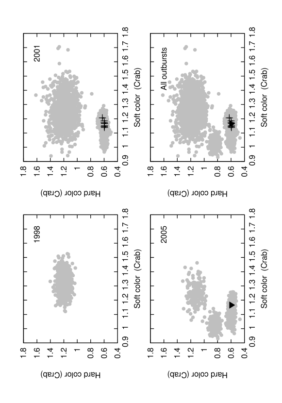
Figure 7: Color-color diagram for the 1998, 2001 and 2005 outbursts (values are normalized by the Crab Nebula, see Section 4.6). Gray circles mark the 16 seconds average color of all available data. Black crosses (2001 outburst) and triangles (2005 outburst) mark the average color per observation in which we find pulsations.

4.7 Radio pulse search

We also used the new phase-coherent timing solution presented here to search for possible radio pulsations from SAX J1748.9$-$2021. For this, we used 2-GHz archival radio data from Green Bank Telescope (GBT) observations of the 6 known radio millisecond pulsars (MSPs) in the globular cluster (GC) NGC 6440 (see Freire et al. 2007 for a description of these data). The known radio pulsars in NGC 6440 have spin periods from 3.8$-$288.6 ms and dispersion measures (DMs) between 219$-$227 pc cm^-3. With a spin period of 2.3 ms, SAX J1748.9$-$2021 is thus the fastest-spinning pulsar known in NGC 6440, where the average spin period of the radio pulsars (11.3 ms when the 288-ms pulsar B1745$-$20 is excluded) is relatively long compared to other GCs.

We searched 11 data sets taken between 2006 December and 2007 March. These data sets have total integration times between $0.5-5$ hr and a combined total time of 20.3 hr (73 ks). The data were dedispersed into 10 time series with trial DMs between 219$-$228 pc cm^-3. To check if pulsations were present, these time series were then folded with the timing solution presented in this paper. Because potential radio pulsations may also be transient, we folded not only the full data sets, but also overlapping chunks of 1/4, 1/10, and 1/50 of the individual data set (thus probing timescales between 100 s and hours). Furthermore, because these data were taken 6 years after the data that was used to construct the timing solution, we folded the data using both the exact period prediction from the timing solution as well as allowing for a small search around this value.

No obvious pulsations were detected in this analysis, where the reduced $\chi^{2}$ of the integrated pulse profile was used to judge if a given fold was worthy of further investigation. This is perhaps not surprising as radio pulsations have, as of yet, never been detected from an LMXB or AMP. Nonetheless, we plan to continue these searches on the large amount of available radio data which we have not yet searched with this technique.

5 Discussion

We have presented a new timing solution for SAX J1748.9$-$2021  obtained by phase connecting the 2001 outburst pulsations. We discovered the presence of timing noise on short (hundred seconds) and long (few days) timescales. We cannot exclude the presence of timing noise on different timescales, since the short and the long timescales found are also the two timescales the TOAs probe. The pulse profiles of SAX J1748.9$-$2021 keep their sinusoidal shape below 17 keV throughout the outburst, but do experience considerable shifts relative to the co-rotating reference frame both apparently randomly as a function of time and systematically with amplitude. Above 17 keV the pulse profiles show deviations from a sinusoidal shape that cannot be modeled adding a 2nd harmonic. The fit needs a very high number of harmonics to satisfactory account the shape of the pulsation. This is probably due to the effect of some underlying unknown non-Poissonian noise process that produces several sharp spikes in the pulse profiles. The lack of a detectable second harmonic prevents us from studying shape variations of the pulse profiles such as was done for SAX J1808.4–3658 (Burderi et al., 2006; Hartman et al., 2007) where sudden changes between the phase of the fundamental and the second harmonic were clearly linked with the outburst phase.
Another interesting aspect is the energy dependence of the pulse profiles, which can be a test of current pulse formation theories. In one model of AMPs, Poutanen & Gierliński (2003) explain the pulsations by a modulation of Comptonized radiation whose seeds photons come from blackbody radiation. The thermal emission is given by the hot spot and/or emitting column produced by the in-falling material that follows the magnetic dipole field lines of the neutron star plasma rotating with the surface of the neutron star. Part of the blackbody photons can be scattered to higher energies by a slab of shocked plasma that forms a comptonizing region above the hot spot (Basko & Sunyaev, 1976).

In three AMPs (Cui et al., 1998; Gierliński & Poutanen, 2005; Poutanen & Gierliński, 2003; Watts & Strohmayer, 2006; Galloway et al., 2007) the fractional pulse amplitudes decreases toward high energies with the soft photons always lagging the hard ones. However in SAX J1748.9$-$2021 the energy dependence is opposite, with the fractional pulse amplitudes increasing toward higher energies and no detectable lags (although the large upper limit of $250\rm\,\mu$s does not rule out the presence of time lags with magnitude similar to those detected in other AMPs). Moreover, all the pulsating episodes happen when the source is in the soft state (although not all soft states show pulsations). This is similar to Aql X-1 (see Casella et al. 2007) where the only pulsating episode occurred during a soft state, and the pulsed fraction also increased with energy. Remarkably all the other sources which show persistent pulsations have hard colors typical of the extremely island state.

Both the energy dependence and the presence of the pulsations during the soft state strongly suggest a pulse formation pattern for these two intermittent sources which is different from that of the other known AMPs and the intermittent pulsar HETE J1900.1-2455. As discussed in Muno et al. 2002, Muno et al. 2003, a hot spot region emitting as a blackbody with a temperature constrast with respect to the neutron star surface produces pulsations with an increasing fractional amplitude with energy in the observer rest frame. The exact variation of the fractional amplitude with energy however has a complex dependence on several free parameters as the mass and radius of the neutron star and the number,size, position and temperature of the hot spot and viewing angle of the observer. The observed slope of 0.2$\rm\,\%\,rms\,keV^{-1}$ is consistent with this scenario, i.e., a pure blackbody emission from a hot spot with a temperature constrast and a weak comptonization (see Falanga & Titarchuk 2007, Muno et al. 2002, Muno et al. 2003). However it is not possible to exclude a strong comptonization given the unknown initial slope of the fractional amplitude.

The pulse shapes above 17 keV are non-sinusoidal and are apparently affected by some non-Poissonian noise process or can be partially produced by an emission mechanism different from the one responsible of the formation of the soft pulses (see for example Poutanen & Gierliński (2003) for an explaination of how the soft pulses can form). We found that the TOAs of the pulsations are independent of the energy band below 17 keV but selection on the fractional amplitude of the pulsations strongly affects the TOAs: high amplitude pulses arrive later. However, this does not affect the timing solution beyond what is expected from fitting other data selections: apparently the TOAs are affected by correlated timing noise. If we take into account the timing noise ($\phi_{N}$) in estimating the parameter errors, then the timing solutions are consistent to within 2$\sigma$. In the following we examine several possibilities for the physical process producing the $\phi_{N}$ term.

5.1 Influence of Type I X-ray bursts on the TOAs

The occurrence of Type I X-ray bursts in coincidence with the appearance of the pulsations suggests a possible intriguing relation between the two phenomena. However as we have seen in §4.4, there is not a strict link between the appearance of pulsations and Type I burst episodes. Only after $\approx 30\%$ of the Type I bursts the pulsations appeared or increased their fractional amplitude. The appearance of pulsations seems more related with a period of global surface activity during which both the pulsations and the Type I bursts occur. This is different from what has been observed in HETE J1900.1-2455 (Galloway et al., 2007) where the Type I X-ray bursts were followed by an increase of the pulse amplitudes that were exponentially decaying with time. We note that during the pulse episodes at MJD 52191.7, 52193.40, 52193.45 and 52195.5 the TOA residuals just before and after a Type I burst are shifted by 300-500$\rm\,\mu$s suggesting a possible good candidate for the large timing noise observed. However in two other episodes no substantial shift is observed in the timing residuals (see Fig. 6). We also note that there is no relation between the Type I burst peak flux and the magnitude of the shifts in the residuals.

5.2 Other possibilities

The timing noise and its larger amplitude in the weak pulses might be related with some noise process that becomes effective only when the pulsations have a low fractional amplitude. Romanova et al. (2007) have shown that above certain critical mass transfer rates an unstable regime of accretion can set in, giving rise to low-$m$ modes in the accreting plasma which produce an irregular light curve. The appearance of these modes inhibits magnetic channeling and hence dilutes the coherent variability of the pulsations. Such a model can explain pulse intermittency by positing that we see the pulses only when the accretion flow is stable. The predominance of timing noise in the low fractional amplitude group could be explained if with the onset of unstable accretion the $m$-modes gradually set in and affect the pulsations, lowering their fractional amplitude until they are undetectable. However the lack of a correlation between pulse fractional amplitude and X-ray flux is not predicted by the model.

Another interesting aspect are the apparent large jumps that we observe in the phase residuals on a timescale of a few hundred seconds. Similar jumps have been observed for example in SAX J1808.4-3658 during the 2002 and 2005 outbursts (Burderi et al. 2006; Hartman et al. 2007. In that case however the phases jump by approximately 0.2 spin cycles on a timescale of a few days, while here we observe phase jumps of about 0.4 cycles on a timescale of hundred seconds. Other AMPs where phase jumps were observed (XTE J1814-338 Papitto et al. 2007, XTE J1807-294 Riggio et al. 2007) have shown timescales of a few days similar to SAX J1808.4-3658. This is a further clue that the kind of noise we are observing in SAX J1748.9$-$2021 is somewhat different from what has been previously observed.

6 Conclusions

We have shown that it is possible to phase connect the intermittent pulsations seen in SAX J1748.9$-$2021 and we have found a coherent timing solution for the spin period of the neutron star and for the Keplerian orbital parameters of the binary.
We found strong correlated timing noise in the post-fit residuals and we discovered that this noise is strongest in low fractional amplitude pulses and is not related with the orbital phase. Higher-amplitude (${\thinspace\hbox to0.0pt{\raise 2.15277pt\hbox{$\scriptstyle{>}$}\hss}{\lower 1.29167pt\hbox{$\scriptstyle{\sim}$}}\thinspace}1.8\%$ rms) pulsations arrive systematically later than lower-amplitude (${\thinspace\hbox to0.0pt{\raise 2.15277pt\hbox{$\scriptstyle{<}$}\hss}{\lower 1.29167pt\hbox{$\scriptstyle{\sim}$}}\thinspace}1.8\%$ rms) ones, by on average 145$\mu$s. The pulsations of SAX J1748.9$-$2021 are sinusoidal in the 5-17 keV band, with a fractional amplitude linearly increasing in the energy range considered. The pulsations appear when the source is in the soft state, similarly to what has been previously found in the intermittent pulsar Aql X-1. The origin of the intermittency is still unknown, but we can rule out a one-to-one correspondence between Type I X-ray bursts and the appearance of pulsations.

References

- Altamirano et al. (2007) Altamirano D., Casella P., et al., Aug. 2007, ArXiv e-prints, 708
- Basko & Sunyaev (1976) Basko M.M., Sunyaev R.A., May 1976, MNRAS, 175, 395
- Bildsten et al. (1997) Bildsten L., Chakrabarty D., et al., Dec. 1997, ApJS, 113, 367
- Burderi et al. (2006) Burderi L., Di Salvo T., et al., Dec. 2006, ApJ, 653, L133
- Casella et al. (2007) Casella P., Altamirano D., et al., Aug. 2007, ArXiv e-prints, 708
- Cordes & Helfand (1980) Cordes J.M., Helfand D.J., Jul. 1980, ApJ, 239, 640
- Cui et al. (1998) Cui W., Morgan E.H., Titarchuk L.G., Sep. 1998, ApJ, 504, L27+
- Falanga & Titarchuk (2007) Falanga M., Titarchuk L., Jun. 2007, ApJ, 661, 1084
- Falanga et al. (2005) Falanga M., Kuiper L., et al., Dec. 2005, A&A, 444, 15
- Freire et al. (2007) Freire P.C.C., Ransom S.M., et al., Nov. 2007, ArXiv e-prints, 711
- Galloway et al. (2005) Galloway D.K., Markwardt C.B., et al., Mar. 2005, ApJ, 622, L45
- Galloway et al. (2007) Galloway D.K., Morgan E.H., et al., Jan. 2007, ApJ, 654, L73
- Gavriil et al. (2007) Gavriil F.P., Strohmayer T.E., et al., Nov. 2007, ApJ, 669, L29
- Gierliński & Poutanen (2005) Gierliński M., Poutanen J., Jun. 2005, MNRAS, 359, 1261
- Groth (1975) Groth E.J., Nov. 1975, ApJS, 29, 453
- Hartman et al. (2007) Hartman J.M., Patruno A., et al., Aug. 2007, ArXiv e-prints, 708
- Hobbs et al. (2006) Hobbs G.B., Edwards R.T., Manchester R.N., Jun. 2006, MNRAS, 369, 655
- in’t Zand et al. (2001) in’t Zand J.J.M., van Kerkwijk M.H., et al., Dec. 2001, ApJ, 563, L41
- Jahoda et al. (2006) Jahoda K., Markwardt C.B., et al., Apr. 2006, ApJS, 163, 401
- Kaaret et al. (2006) Kaaret P., Morgan E.H., et al., Feb. 2006, ApJ, 638, 963
- Kuulkers et al. (1994) Kuulkers E., van der Klis M., et al., Sep. 1994, A&A, 289, 795
- Muno et al. (2002) Muno M.P., Özel F., Chakrabarty D., Dec. 2002, ApJ, 581, 550
- Muno et al. (2003) Muno M.P., Özel F., Chakrabarty D., Oct. 2003, ApJ, 595, 1066
- Papitto et al. (2007) Papitto A., di Salvo T., et al., Mar. 2007, MNRAS, 375, 971
- Pooley et al. (2002) Pooley D., Lewin W.H.G., et al., Jul. 2002, ApJ, 573, 184
- Poutanen & Gierliński (2003) Poutanen J., Gierliński M., Aug. 2003, MNRAS, 343, 1301
- Riggio et al. (2007) Riggio A., Di Salvo T., et al., Oct. 2007, ArXiv e-prints, 710
- Romanova et al. (2007) Romanova M.M., Kulkarni A.K., Lovelace R.V.E., Nov. 2007, ArXiv e-prints, 711
- Rots et al. (2004) Rots A.H., Jahoda K., Lyne A.G., Apr. 2004, ApJ, 605, L129
- Taylor (1992) Taylor J.H., 1992, Philosophical Transactions of the Royal Society of London, 341, 117-134 (1992), 341, 117
- van Straaten et al. (2003) van Straaten S., van der Klis M., Méndez M., Oct. 2003, ApJ, 596, 1155
- Watts & Strohmayer (2006) Watts A.L., Strohmayer T.E., Dec. 2006, MNRAS, 373, 769