The comet 17P/Holmes 2007 outburst: the early motion of the outburst material.

Abstract

Context. On October 24, 2007 the periodic comet 17P/Holmes underwent an astonishing outburst that increased its apparent total brightness from magnitude $V\sim 17$ up to $V\sim 2.5$ in roughly two days. In this contribution we report on Wendelstein $0.8\,$m telescope (WST) photometric observations of the early evolution stages of the outburst.

Aims. We studied the evolution of the structure morphology, its kinematic, and provided an estimate of the ejected dust mass.

Methods. We analized $126$ images of the comet in the $BVRI$ photometric bands spread between 26 October, 2007 and November 20, 2007. The bright comet core appeared well separated from that one of a quickly expanding dust cloud in all the data, and the bulk of the latter was contained in the field of view of our instrument during the days soon after the outburst, allowing precise estimates both of the separation velocities of the two luminous baricenters, and of the expansion velocity of the dust cloud. The ejected dust mass was derived on the base of differential photometry on background stars occulted by the moving cloud.

Results. The two cores were moving apart from each other at a relative projected constant velocity of $(9.87\,\pm\,0.07)\,$arcsec/day ($0.135\,\pm\,0.001$ km/sec). In the inner regions of the dust cloud we observed a linear increase in size at a mean constant velocity of $(14.6\,\pm\,0.3)\,$ arcsec/day ($0.200\,\pm\,0.004\,$ km/sec). Evidence of a radial velocity gradient in the expanding cloud was also found. Our estimate for the expanding coma’s mass was of the order of $10^{-2}-1\,$ comet’s mass implying a significant disintegration event.

Conclusions. We interpreted our observations in the context of an explosive scenario which was more probably originated by some internal instability processes, rather than an impact with an asteroidal body. Due to the peculiar characteristics of this event, further observations and investigations are necessary in order to enlight the nature of the physical processes that determined it.

1 Introduction

In this Letter, we concentrate on the analysis of the outburst of comet 17P/Holmes, occurred on October 24, 2007 (Santana 2007). We provide an overview analysis of the early evolution phases of the surrounding cometary environment, in the period between October $26$, $2007$ and November $20$, $2007$ considering the global structure of the expanding material, its kinematic properties and inferring the ejected dust mass. Comet brightenings are well documented in the literature, and in general they can be associated with either evident cometary nuclear fragmentation or not (see e.g. Sekanina et al. 2002 and references therein). Despite their recurrence, the magnitude and the characteristics of the outbursts occurring to comet 17P/Holmes largely justify its longstanding reputation in the annals of astronomy (Barnard 1896). The periodic comet 17P/Holmes was discovered on November 6, 1892 by E. Holmes in London, during an outstanding brightness increase, followed by another similar event on January 16, 1893. When discovered by Mr. Holmes the comet was around $5$ months past perihelion $(\rm T\,=\,$June 13). On October 24, 2007 around $6$ months after the last perihelion passage $(\rm T\,=\,$May 4, 2007) the comet underwent a similar phenomenon to those observed more than one hundred years ago. The heliocentric distance of the object at the time of the two major events was around $\rm\Delta_{sun}\,=\,$2.39 AU and $\rm\Delta_{sun}\,=\,$2.44 AU in 1892 and 2007 respectively, and the orbital inclination remained substantially unaltered during this period ($\rm i\,\sim\,20^{\circ}$). This Letter is structured in the following way: in Sect. 2, we present the observations we acquired, and the data reduction method. In Sect. 3, we discuss the morphological evolution of the expanding structure. In Sect. 4, we calculated the separation velocities between the comet and the center of the dust cloud, as well as the expansion velocity of the cloud. In Sect. 5, we estimated the ejected dust mass. Finally in Sect. 6, we sum up our results.

2 Observations and reduction of the data

The observations were acquired on October 26/28/29/31, 2007 and November 2/5/20, 2007. A total number of $126$ images were analized in the $BVRI$ filters. An overview of the observations is shown in Tab. 1. The images were acquired using the MONICA CCD camera, at the Cassegrain focus of the 0.8 m Wendelstein telescope, with a scale of $0.5\,$arcsec/pix, and a field of view of around $8\,$x$\,8\,$ arcmin. The pre-reduction process was done using standard reduction software (MUPIPE) specifically developed at the Munich Observatory for the MONICA CCD camera (Gössl & Riffeser 2002). The weather conditions were in general clear for all our observing nights with the exception of night 26, which was cloudy. Otherwise we were able to acquire $1$ image in the $R$ band during that night, and to use it for the analysis of the kinematic properties of the cloud described in Sect. 4. The exposure times were comprised between $40$ and $200$ sec for the whole dataset.

Table 1: Number of images of 17P/Holmes taken during the different observing nights in the $BVRI$ filters.

DATE	$B$	$V$	$R$	$I$
26/10/2007	-	-	$1$	-
28/10/2007	$6$	$6$	$9$	$11$
29/10/2007	$10$	$5$	$10$	$10$
31/10/2007	$10$	-	$12$	$13$
02/11/2007	$4$	$3$	$5$	-
05/11/2007	-	-	$5$	-
20/11/2007	-	-	$6$	-

During night 28, the photometric conditions were good and stable over the whole night, and we thus acquired some images of the Landolt standard field PG0918 in all our filters. We obtained $2$ images in the $B$, $V$, $R$ bands, and $4$ images in the $I$ band. These data were reduced exactly in the same manner as the scientific observations (see also Sect. 5). The magnitudes of the standard stars were reported to $1$ airmass and $1$ arcsec, and finally calibrated to the Landolt photometric system, thanks to the Stetson Photometric Standard Fields  data of PG0918. We found a total of $26$ common stars between our catalog and that one provided by Stetson, and obtained the following calibration equation for the $R$ band against the $V-R$ color:

$$R\,-\,r\,=\,-0.07\,(\pm\,0.02)\,(V\,-\,R)\,+\,23.18\,(\pm\,0.01)$$

The $\rm RMS$ residual of the fit with respect to the best fitting least square linear model was $\sim 0.02\,$mag. This result gives an idea of our photometric precision during that night, and will be useful in Sect. 5, in the discussion of the ejected mass estimate.

3 The evolution of the morphological structure

In order to show the evolution of the morphological structure of the object, we selected for each night in our dataset one representative image in the $R$ band. These images were scaled to the same exposure time, airmass and intensity range, in order to properly sample the surface brightness of the coma on the whole dataset. The lowest intensity level was chosen close to the lowest counts we got on the last image of our dataset, while the highest close to the coma’s peak intensity of the image taken on October 28, 2007. We did not process in this way the image acquired on October 26, 2007, because it was too noisy. The images were then normalized to the lowest intensity level. Finally, we displayed the images codified on a logarithmic color scale, as shown in Fig. 1. We overplotted to each panel the isophote intensities levels, to highlight the structure of the inner part of the cloud. The most interesting feature of Fig. 1 is the presence of two bright cores (the comet core beeing towards the upper left side). These two cores were increasingly separating during the observing period and appeared elongated towards each other, indicating an exchange of mass between them. Moreover the expansion of the global structure is evident from the sequence of images. We also displayed the intensity value of the closest isophote to the cloud’s center, and of the adjacent one in the outwards direction. The exact values given by the isophotes depends on the adopted number of isophotes in each panel, which determines also the intensity step between them. We set the number of isophotes in order to provide approximately the same sampling of the inner regions of the cloud. Thus, the quoted numbers must be considered as indicative of the relative surface brightnesses of the cloud in the different nights. The intensity of the innermost isophote of night $28/11/2007$ was around $2$ orders of magnitude larger with respect to the correpondent isophote’s intensity of night $20/11/2007$, and the intensity step between the isophotes was also $1$ order of magnitude larger in the first case with respect to the second. We underline that there is no way to significantly change these conclusions adopting different isophotal mapping criteria, as we accurately verified. Actually, both these results are the consequence of the rapid expansion of the dust cloud, which determines a steady decrease of its surface brightness, and a more homogeneous light distribution in the more evolved, and less concentrated phases.

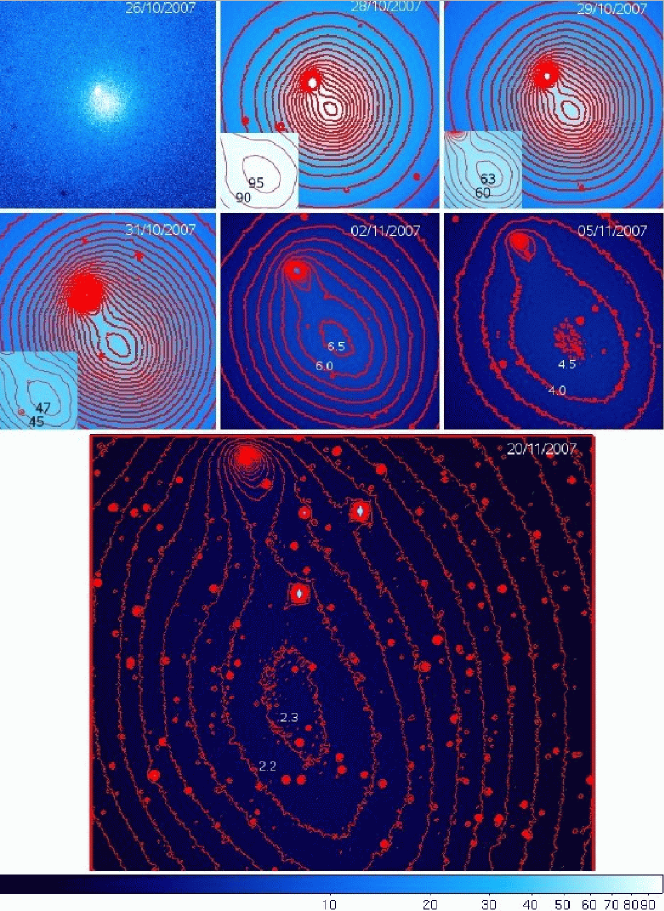
Figure 1: Snapshot of $R$ band images acquired during each night of our observing run, showing the evolution of comet 17P/Holmes’ morphological structure. Each image has been scaled to the same exposure time, airmass, intensity range, and displayed on a logarithmic color scale, codified by the bottom color bar. The top $6$ images are zoomed inside the inner regions of the object, and have a field of view of $2.2\,$x$\,2.2$ arcmin, whereas the last one of $8\,$x$\,8$ arcmin. Two cores are visible in all the images, the comet nucleus (on the upper left side) and that one of the coma, rapidly separating during the observing period. The values reported on the coma’s innermost isophotes of each panel (or in the close-up views of 28/29/31 nights) put in evidence the surface brightness decrement of the coma due to its rapid expansion.

4 Kinematic of the expanding materials

In this Section we derived the separation velocity of the two bright baricenters, and the dust cloud’s expansion velocity. The comet’s center appeared in all our images as a point-like source, thus the peak’s position was derived with a gaussian fitting algorithm, as done for stellar objects. The light distribution of the dust cloud was extended over a much larger area and was not gaussian overall, but we found that the inner part could be always represented by a gaussian. We thus fit a bidimensional gaussian using the light distributions along the x and y axis. An initial guess for the centroid was provided with a maximum finding algorithm run in a small region around the peak ($\sim\,30\,$arcsec). Then a least square fit provided the refined position for the centroid, and the $\sigma_{x}$ and $\sigma_{y}$ of the fitting gaussians. In Fig. 2 (left panel) we plotted the two bright cores’ projected distances against the Julian Date (JD) of the observations. The correction for the Earth’s variable distance has been taken into account, although negligible. We obtained a uniform increasing separation with a mean velocity of $(9.87\,\pm\,0.07)$ arcsec/day ($0.135\,\pm\,0.001$ km/sec). The uncertainties are dominated by the errors in the diffuse cloud centroids. In the right panel of Fig. 2, we reported the $\sigma$ of the diffuse clouds (actually the mean of the $\sigma_{x}$ and $\sigma_{y}$) as a function of the JD. We did not include in this Figure the last two nights, because the cloud was too expanded. Two images acquired on night $2/11/2007$ in the $R$ band were also excluded because of the large offset of the cloud’s centroid with respect to the image’s center. The errorbars in this Figure are calculated as the difference of the $\sigma$ along the x and y axis. The different colors in the figure codify observations obtained in the different photometric bands, respectively black for $B$, blu for $V$, red for $R$, and yellow for $I$. Also in this case we observed a linear increase in size with a mean velocity of $(14.6\,\pm\,0.3)$ arcsec/day ($0.200\,\pm\,0.004\,$ km/sec). Repeating the calculation separately for the different bands gave the result in Tab. 2. These mean values and their errors were obtained using a weighted least square algorithm. The different bands allow to explore different layers of the expanding cloud, more external in the $B$, and deeper in the redder bands. Thus, this result can be interpreted as the evidence of a radial velocity gradient in the expanding cloud. For each couple of adiacent bands we considered the ratio between the difference of the expansion velocities reported in Tab. 2, and the difference in the correspondent $\sigma$ values given by the least square fitting models for the night 2/11/2007, for which we obtained the largest separation among the expanding shells. Taking the mean of these values we obtained an estimate of the radial velocity gradient during that night equal to $\rm(0.3\,\pm\,0.2)\,10^{-5}\,sec^{-1}$ which means an increase of around $0.3\,$cm/sec every km going from the center to the surface of the coma.

All these kinematic observations could be explained in the context of an explosive scenario. While, as a consequence of the explosion, a part of the cometary nucleus was disintegrated and the material was outflowed in all directions resulting in the sperically symmetric expanding coma, the survived nucleus received a kick separating from the coma’s center with the observed projected velocity. The expansion velocity of a particle of radius $a$ during an explosive event is proportional to $a^{-1}$ (see e.g. the discussion in Tozzi et al. 2007) implying a higher expansion velocity for the smaller, less massive particles with respect to the larger and more massive ones, which resulted in the observed velocity gradient in the expanding cloud.

The formation of spherical expanding envelopes around the cometary nucleus of 17P/Holmes was observed for both the events occurred in November 1892 and in January 1893. Bobrovnikoff (1943) compared the observations obtained by different authors between 16-22 January 1893, deriving a uniform expansion velocity of $(0.54\,\pm\,0.03)\,$km/sec, thus similar to what found here. The sudden brightness increases, the formation of spherical dust envelopes with similar kinematic properties, the correspondence in the orbital phase at the instant of the major outbursts noted in Sect. 1, point towards a common mechanism at the base of the observed phenomena. Moreover, the distance from the ecliptic plane was in both cases around $0.8\,$AU. Given that, although it cannot be completely excluded, it seems unlikely that the above mention explosive mechanism was prompt by an asteroidal impact, beeing thus more probable an internal instability process .

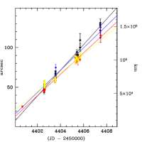
Figure 2: Left: angular projected distance between the centroid of the two bright baricenters, for all the images in our dataset, against the $\rm JD$ of the observations. The continuous line denotes the best fit linear model. On the left hand y-axis values are in arcsec, whereas on the right hand y-axis values are in km. Right: $\rm\sigma$ of the expanding cloud gaussian core against $\rm JD$. Different colors indicate measurements obtained in different bands: $B$ in black, $V$ in blue, $R$ in red and $I$ in yellow. The best fit linear models in each band are represented by the continuous lines.

Table 2: The derived expansion velocities in arcsec/day along with their uncertainties for the expanding dust cloud in the different bands. In parenthesis we report the correspondent values in km/sec.

Filter	Expansion vel.	$\pm$	err
$B$	16.2(0.222)		0.5(0.007)
$V$	14.0(0.193)		0.6(0.009)
$R$	13.5(0.185)		0.2(0.003)
$I$	11.9(0.163)		0.4(0.005)

5 The ejected mass estimate

In the following we provide an estimate of the ejected dust mass during the outburst, through the extinction produced by the dust cloud on the surrounding background stars. We selected two well exposed, good seeing images taken on October 28, 2007 in the $R$ filter. These images had the largest time separation ($2$ hours) in the whole dataset, among equal filter images acquired during the same observing night. Thus, they provided the largest apparent motion of the cloud on the sky plane. At the same time, this temporal difference is small enough to avoid the expansion of the cloud to change significantly the extinction map, allowing an homogeneous comparison of the two images. Finally, day 28 was as close to the outburst as to allow the dust cloud to fit well inside our field of view. We performed PSF fitting photometry with DAOPHOT/ALLSTAR (Stetson 1987) and rejected all the stars with $\chi>1.5$ and absolute $sharp$ values bigger than $1$. These parameters and selection criteria allowed to exclude those objects for which a reliable fit of the stellar model couldn’t be performed, because close to saturation, bad pixels, and to reject non-stellar sources like cosmic rays or background galaxies, spikes of saturated stars etc. The sky background in these images was estimated locally around each star, in an annular region comprised between $1.5$ and $3.5$ arcsec from the stars’ centroids. This region was selected after performing different tests looking at the best subtraction of the analized stars. The modal value of the pixel counts inside the selected annular region was considered as the estimate of the sky background. The photometry was extracted in a circular region centered on the stars’ centroids with radius equal to $1.3\,$arcsec, which corresponded to the seeing value in both the images. The derived magnitudes were then reported to $1$ airmass and $1\,$ sec of exposure time for both the images. We then consider all the common objects with radial distance from the center of the comet $>25$ arcsec, and with radial distance from the center of the cloud $<3$ arcmin in both the images. The inner limit was necessary to avoid the photometry of the stars to be biased by the luminous core of the comet. The outer limit was chosen to avoid detector border effects, accounting for the position of the center of the cloud in both the images. At the end, we obtained a catalog of $20$ stars spread inside the analized region of the cloud, see Fig. 3.

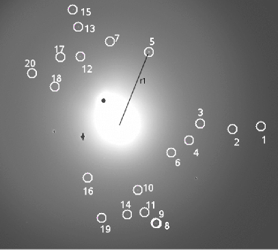
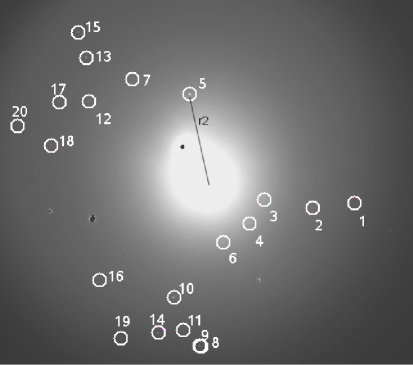
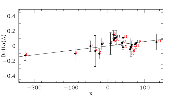
Figure 3: Top: spatial distribution of the $20$ background stars used in Sect. 5 to probe the differential extinction produced by the coma, for the two images acquired on October 28, 2007. The image on the left was taken $2$ hours before the right one. The selected stars are indicated by white circles. The associated numeration corresponds to that one in the lower panel, allowing to relate each star to the correspondent measured differential extinction. Bright sources were saturated (black regions), as well as the center of the cometary nucleus. The black lines indicate the distances, referred in Sect. 5 as $\rm r_{1}$ and $\rm r_{2}$, of one star with respect to the estimated coma’s centers. Bottom: the correlation between the differential extinctions in the $R$ band ($\rm\Delta\,A$), and the $\rm x$ parameter (see text for details).

In order to demonstrate the radial dependence of the extinction from the center of the cloud, we assumed a uniform and homogeneous spherically symmetric mass distribution. Thus, being $\rm r$ the position of one star with respect to the cloud’s center, we can express the optical depth of the cloud at the distance $\rm r$ as:

$$\rm\tau(r)=\sigma_{d}\,n\,2\sqrt{\rm R^{2}-r^{2}}$$ (1)

where $\rm 2\sqrt{R^{2}-r^{2}}$ is the lenght of the segment of sphere with projected distance $\rm r$, with respect to the cloud’s center, $\rm R$ is the radius of the cloud, $\rm\sigma_{d}$ is the cross section of the dust grains in a given observing band, and $\rm n$ is the number density of the dust particles. Considering two different positions $\rm r_{1}$ and $\rm r_{2}$ of a generic star in the first and in the second image with respect the cloud’s center we can express the differential extinction $\rm\Delta\,A$, produced by the cloud in the two positions as:

$$\rm\Delta\,A\,\,\,=\,\,\,m_{1}\,-\,m_{2}\,=\,-2.5\,\log\left(\frac{I_{1}}{I_{2}}\right)=\,-2.5\,log\left[\frac{e^{-\sigma_{d}\,n\,2\,\sqrt{\rm R^{2}-r_{1}^{2}}}}{e^{-\sigma_{d}\,n\,2\,\sqrt{\rm R^{2}-r_{2}^{2}}}}\right]$$ (2)

which implies:

$$\rm\Delta\,A\,\,\,\,=\,\,\,(2.5\,\sigma_{d}\,n\,2\,\log\,e)\,\Big{(}\sqrt{\rm R^{2}-r_{1}^{2}}-\sqrt{\rm R^{2}-r_{2}^{2}}\Big{)}\,\,\,\,=$$

$$\rm\,\,\,\,\,\,\,\,\,\,\,\,\,\,\,=\,\,\,\,\alpha\,\,\,\,\Big{(}\sqrt{\rm R^{2}-r_{1}^{2}}-\sqrt{\rm R^{2}-r_{2}^{2}}\Big{)}$$ (3)

where $\rm m_{1}$,$\rm I_{1}$ and $\rm m_{2}$,$\rm I_{2}$ are the $observed$ magnitudes (intensities) of the star at the position $\rm r_{1}$ and $\rm r_{2}$ respectively. As easily recognized, this model satisfies the required simmetry conditions with respect to $\rm r_{1}$ and $\rm r_{2}$. Actually, if $\rm r_{1}$ is equal to $\rm r_{2}$, the differential extinction should be zero. Morever, if we consider two stars with initial $\rm r_{1}$, $\rm r^{{}^{\prime}}_{1}$, and and final $\rm r_{2}$, $\rm r^{{}^{\prime}}_{2}$ positions respectively, that satisfy the condition $\rm r_{1}=r^{{}^{\prime}}_{2}$ and $\rm r_{2}=r^{{}^{\prime}}_{1}$, the resulting differential extinctions for the two stars should be equal and opposite in sign. In particular $\rm\Delta\,A$ should be positive when $\rm r_{1}<r_{2}$, (the star is moving away from the cloud center, and thus is less extincted in $\rm r_{2}$ with respect to $\rm r_{1}$), and negative when $\rm r_{1}>r_{2}$ (the star is going towards the cloud center). This implies that the angular coefficient $\rm\alpha$, in Eq. 3, should be positive. The value of $\rm\alpha$ gives the extinction for unitary length in the given observing band. Therefore, we fit to the observed differential extinctions the model:

$$\rm\Delta\,A\,=\,\alpha\,x\,+\beta$$ (4)

where $\rm x=\sqrt{\rm R^{2}-r_{1}^{2}}-\sqrt{\rm R^{2}-r_{2}^{2}}$, and the $\rm\beta$ coefficient was included to account for residual constant zero points between the two images. The result, after subtracting the constant zero point, is shown in the bottom panel of Fig. 3. We found a positive correlation between the differential extinction $\rm\Delta\,A$, and the $\rm x$ parameter, as expected. The derived value of the $\rm\alpha$ coefficient was $(0.0006\,\pm\,0.0002)\,$mag/pix, where a pixel corresponds to around $592\,$km at the distance of the comet. This value has been obtained assuming a radius $\rm R$ for the cloud of $3\,$arcmin ($\rm\sim\,3.5\,\rm\sigma$ for that night for the luminous distribution analized in Sect. 4). Increasing the radius to $4\,$arcmin ($\rm\sim\,5\,\rm\sigma$) implies a value of $\rm\alpha\,=\,(0.0012\,\pm\,0.0004)\,$mag/pix.

The most important assumptions of the model are the dust cloud’s spherical geometry and the homogeneous and uniform mass distribution. The geometry of the cloud was well constrained by the observations and the analysis presented in the previous Sections. As for the second hypothesis, it allowed to express the optical depth in a straightforward and convenient way, as shown in Eq. 1, and ultimately implies the linear dependence of the observed differential extinctions on the geometrical factor $x$. A strong deviation from that assumption would imply a strong deviation from the linear model prediction, which is not observed (Fig. 3). The scatter in that relation ($\sim 0.06\,$ mag) is larger than the scatter derived from the calibration of the Landolt standard field discussed in Sect. 2 ($\sim 0.02\,$ mag). Otherwise, in the science images the surface brightness of the coma determined a background around $10$ times larger than in the Landolt images, which explains the factor of $3$ increase in the scatter. The radial velocity gradient of the expanding material discussed in Sect. 4 points against the uniform mass distribution hypothesis. Otherwise, as shown in the right panel of Fig. 2, during night $28$ the expanding shells were certainly more concentrated together than in the later evolved phases beeing that night closer to the outburst. In conclusion, it is reasonable to believe that in the chosen night the material was not far from beeing uniformly distributed and homogeneously mixed and we considered this hypothesis as a good approximation of the structural properties of the observed coma. Therefore, the dominant factor that explains the observations is related to the cloud’s geometrical structure, in the sense that the observed differential extinctions were determined by the variable quantity of mass over the cloud’s different line of sights probed by the background stars (directly implied by its spherical structure). This is overall demonstrated by the observed linear dependence of the differential extinction from the geometrical factor x, and by the positive value of the $\alpha$ coefficient, also predicted by the model.

To derive the coma’s mass we considered spherical dust grains with a mean density $\rm\rho_{d}$ ($\rm=2.5\,g/cm^{3}$) and a ’typical’ dimension $\rm r_{d}$ (and thus mass $\rm m_{d}=4/3\,\pi\,r_{d}^{3}\,\rho_{d}$). Thanks to the definition of the $\rm\alpha$ parameter in Eq.3, the mass of the cloud $\rm M$ can be expressed through the following formula:

$$\rm M=\frac{4}{3}\,\pi\,R^{3}\,m_{d}\,n=\frac{4}{3}\,\pi\,R^{3}\,\left(\frac{4}{3}\,\pi\,r_{d}^{3}\,\rho_{d}\right)\left(\frac{\alpha}{5\,\sigma_{d}\,\log\,e}\right)=$$

$$\rm\,\,\,\,\,\,\,\,=\frac{16\,\pi}{45\,\log\,e}\,R^{3}\,r_{d}\,\rho_{d}\,\alpha,\simeq\,R^{3}\,r_{d}\,\rho_{d}\,\alpha$$ (5)

where the grain’s cross-section was taken equal to the geometrical cross-section $\rm\sigma_{d}\,=\,\pi\,r_{d}^{2}$ and the numerical factor is $\sim\,2.6$. We varied the value of $\rm r_{d}$ inside a range of characteristic grain dimensions, $\rm 0.005-1\,\mu$m (Mathis et al. 1977), and the dimension of the cloud $\rm R$ between $3-4\,$arcmin. The derived estimate for the coma’s mass was comprised between $10^{12}-10^{14}$kg. Snodgrass et al. (2006) provided the most recent values for this comet’s dimension and density. In particular, from their time-series photometry they obtained a value for the effective radius of the nucleus (Russel 1916) of $\rm(1.62\,\pm\,0.01)\,km$. Even if accurate, this estimate is based on the assumption that the geometrical albedo was equal to $\rm A_{R}=0.04$. Furthermore, they derived a comet’s minimum density equal to $\rm\rho\,=\,0.09\,g/cm^{3}$. Assuming thus a range of possible densities ($\rm\rho\,=\,0.1-1\,g/cm^{3}$) and albedos ($\rm A_{R}\,=\,0.01-0.1$) and using Eq. $\rm(1)$ in Snodgrass et al. (2006) to derive the correspondent effective radii, we obtained a total nuclear mass comprised between $10^{12}-10^{14}$kg. Given the uncertainty range in our mass estimate we concluded that the probable value of the expanding coma’s mass resulting from the outburst event was comprised between $10^{-2}-1$ comet’s mass.

There are different factors that could affect our result. Dust grains in cometary ejecta typically span a range of different dimensions and optical properties (see e.g. Lisse et al 2007, Tozzi et al. 2007). Anyway, both the assumption on the uniform and homogeneous mass distribution, and the lack of specific observations able to constrain the dust population characteristics for this particular object, justify our simplified approach to summarize the cloud’s grain content assuming a ’typical’ grain dimension and the correspondent geometrical cross-section. Another possible drawback in our coma’s mass estimate regards the pre-outburst activity of the comet. During the most recent observations of the comet obtained before the outburst (Snodgrass et al. 2006) the object appeared to be inactive, although the heliocentric distance at that time was $\sim 4.66\,$AU, whereas at the outburst $\sim 2.44\,$AU. Moreover, it seems probable that the explosive event described in this work largely overcame the common activity of the comet. Finally, the stars used to probe the differential extinction produced by the coma (Fig. 3), were well distributed inside the coma, avoiding the region close to the comet’s nucleus, and thus reflecting more closely the contribution to the differential extinction of the material coming directly from the explosion.

Despite the above mentioned approximations, the result presented in Eq. 5, has the advantage to be simple, to enlight the dependence among the total mass of the cloud, the cloud’s geometrical, composition properties and the observed differential extinctions, and to provide an estimate for the expanding coma’s mass which points towards a consistent disintegration phenomenon, as suggested by the large outburst event.

6 Conclusions

In this Letter we analized the early phases of the outburst that comet 17P/Holmes underwent on October 24, 2007. We acquired $BVRI$ photometric images at the Wendelstein $0.8\,$m telescope, between 26/10/2007 and 20/11/2007. We observed a spherically simmetric dust cloud moving away from the comet nucleus with a mean projected constant velocity of $(9.87\,\pm\,0.07)$ arcsec/day ($0.135\,\pm\,0.001$ Km/sec), while the dust cloud was expanding with a mean constant velocity of $(14.6\,\pm\,0.3)$ arcsec/day ($0.200\,\pm\,0.004\,$ Km/sec). These results are in agreement with the ones obtained during past outbursts of this comet. Evidence of a gradient in the expansion velocity of the dust cloud was also found with the velocity increasing towards the external regions. Finally, performing differential photometry on background stars occulted by the moving cloud, and assuming a uniform and homogeneous spherical mass distribution, we derived for the coma’s mass a value of $10^{12}-10^{14}$kg, around $10^{-2}-1$ comet’s mass. We interpreted our observations in the context of an explosive event, probably caused by some internal instability processes, rather than by an asteroidal body’s impact. Various mechanisms have been proposed in the past to explain comets’ splitting, involving tidal, thermal and rotational forces (Sekanina 1997). These processes could have played an important role for the event discussed here, although some specific characteristics allow to consider it as more peculiar. For example, generally the separation velocities of the splitting components are of the order of a few $\rm m/s$, while in this case we found a projected relative velocity around $2$ orders of magnitude larger. The outburst itself represents the largest apparent brightness increase ever observed for a comet. In conclusion, we underline the importance to consider other observational results in order to accurately characterize this event and to provide a more insight view on its enigmatic and still not well understood nature.

- (1) Barnard E. E. 1896, ApJ, 3, 41
- (2) Bobrovnikoff N. T. 1943, PA, 51, 542
- (3) Gössl., C. A. & Riffeser, A. 2002, A&A, 381, 1095
- (4) Lisse, C. M. et al. 2007, Icarus, 191, 223
- (5) Mathis, J. S. et al. 1977, ApJ, 217, 425
- (6) Russell, H. N. 1916, ApJ, 43, 173
- (7) Santana, A. H. 2007, IAU Circ., 8886
- (8) Sekanina, Z. 1997, A&A, 318, 5
- (9) Sekanina, Z. et al. 2002, ApJ, 572, 679
- (10) Snodgrass, C., Lowry, S. C., Fitzsimmons, A., 2006, MNRAS, 373, 1590
- (11) Stetson, P. B. 1987, PASP, 99, 191
- (12) Tozzi, G. P. et al. 2007, A&A, 476, 979