Invisible sunspots and rate of solar
magnetic flux emergence

Abstract

Aims. We study the visibility of sunspots and its influence on observed values of sunspot region parameters.

Methods. We use Virtual Observatory tools provided by AstroGrid to analyse a sample of 6862 sunspot regions. By studying the distributions of locations where sunspots were first and last observed on the solar disk, we derive the visibility function of sunspots, the rate of magnetic flux emergence and the ratio between the durations of growth and decay phases of solar active regions.

Results. We demonstrate that the visibility of small sunspots has a strong centre-to-limb variation, far larger than would be expected from geometrical (projection) effects. This results in a large number of young spots being invisible: 44% of new regions emerging in the west of the Sun go undetected. For sunspot regions that are detected, large differences exist between actual locations and times of flux emergence, and the apparent ones derived from sunspot data. The duration of the growth phase of solar regions has been, up to now, underestimated.

1 Introduction

The birth of a new spot on the solar disk indicates the emergence of magnetic flux through the photosphere, a process which is key to the solar cycle Solanki (2003); Fisher et al. (2000) and the study of stellar magnetic dynamos. Sunspots also cause variations in the total solar irradiance, an important parameter in determining the Sun’s influence on climate Foukal et al. (2006). The presence of a sunspot is key to a solar region being assigned an active region number by the NOAA Space Weather Prediction Center (http://www.swpc.noaa.gov) so that its evolution and activity can be tracked Gallagher et al. (2007). The formation and evolution of active regions are fundamental to solar dynamic phenomena such as flares and Coronal Mass Ejections and their effect on the Earth environment.

The visibility of sunspots is currently thought to be limited only by geometrical effects arising from projection of the solar sphere onto a 2D image, effects referred to as foreshortening. In this paper we present results obtained serendipitously while analysing sunspot data by means of Virtual Observatory tools, showing that the visibility of small sunspots is much poorer than predicted by the foreshortening model.

2 Data analysis

We analysed sunspot group data from the USAF/Mount Wilson catalogue, for times between 1 December 1981 to 31 December 2005, covering two and a half solar cycles. We processed the data by means of AstroGrid workflows. AstroGrid (http://www.astrogrid.org) Walton et al. (2006) is the UK’s contribution to a global Virtual Observatory (VO), aimed at allowing seamless access to a variety of astronomical data, and at providing efficient software tools for data analysis. Our workflows processed all entries in the catalogue and extracted properties of individual regions, identified by their NOAA region number, including the time and location of their first and last observation. The longitude of each region at 12:00UT on the days when it was first and last observed was calculated.

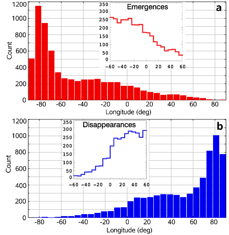
Figure 1: Histograms of number of sunspot regions versus their longitude at 12:00 UTC on the day when they were first (a) and last (b) observed . Each longitude bin is 6^∘. Data are from the USAF/Mt Wilson catalogue of sunspot groups, for the time range 1 December 1981 to 31 December 2005. The total number of regions is 6862. Longitude 0^∘ corresponds to the Earth-Sun line, negative values to eastern longitudes and positive values to western longitudes. Insets show the histograms for the range [$-$60^∘, $+$60^∘].

Figure 1 shows histograms of the locations at which sunspot regions were first and last observed, with 0^∘ longitude corresponding to the Earth-Sun line. As the Sun rotates, many spots first come into view near the east (or ‘rising’) limb, causing the peak to the left in Fig. 1-a. Similarly, the peak in Fig. 1-b corresponds to regions that rotated out of view. Regions first observed sufficiently far from the east limb, are generally assumed to be ‘new’, indicating the emergence of magnetic flux through the photosphere. As spots move in longitude by approximately 14.3^∘ each day, regions first observed to the west of $-$60^∘ are typically described as new emergences (see inset in Fig. 1-a). Similarly regions last seen to the east of $+$60^∘ are interpreted as having decayed to the point that a spot is no longer visible (see inset in Fig. 1-b).

The insets in Fig. 1 display strong east-west asymmetry. A total of 825 new regions are seen to emerge in the bin [$-$60^∘,$-$40^∘], while only 177 in [$+$40^∘,$+$60^∘], a ratio of 4.7:1. What is the cause of the strong asymmetry in these curves? Why should the number of new regions emerging in any given longitude bin not be constant? What is the true rate of magnetic flux emergence on the Sun?

An asymmetry in the location of emergence of new sunspots as viewed from Earth was discovered 100 years ago Maunder (1907) and attracted the attention of famous physicists, who demonstrated that a visibility function that favours observations in the centre of the disk, and the curve of evolution of a spot’s size, can produce such asymmetry Schuster (1911); Minnaert (1939). The graphical representation introduced by Minnaert (1939) makes the cause of the asymmetry immediately clear. However, Minnaert himself went on to assume that the only factor limiting the visibility of sunspots is geometrical effects associated with foreshortening. This results in a visibility function proportional to $\sec{\lambda}$, with $\lambda$ the longitude, and poor visibility only very near the limb. The latter assumption has remained undisputed until the present day. Moreover, appreciation of the cause of the east-west asymmetry appears to have been lost, and asymmetries in sunspot parameters have since been ascribed, e.g., to observer bias or systematic inclination of the magnetic flux tubes Howard (1991).

The large asymmetries in the insets of Fig. 1, however, demonstrate that the visibility of new sunspot formation in [$-$60^∘, $+$60^∘] is poor, and flux appears to emerge and disperse at locations (and times) that are far from the locations (and times) where actual emergence and decay took place.

We use the data of Fig. 1 to derive the rate of region emergence, the average ratio between the slopes of growth and decay phases of region evolution and to determine the visibility function. Let $s(\lambda)$ be the visibility function, giving the minimum actual (as opposed to apparent) area that a sunspot region needs to reach to be visible at longitude $\lambda$. $s$ is expected to have a minimum at $\lambda$=0, where visibility is best. Assuming that, over a given time period, the number of magnetic flux emergences in a unit longitude bin is a constant $N_{1}$, the number $N(\lambda)$ of regions observed emerging in a unit bin at longitude $\lambda$ is Schuster (1911) [See also Appendix A]:

$$N(\lambda)=N_{1}\,\left[1-\frac{\Omega}{k}\,s^{\prime}(\lambda)\right]$$ (1)

where $\Omega$ is the solar rotation rate and $k$ is the linear growth constant of a region’s area with time. Similarly, we obtain for the number $n(\lambda)$ of regions seen to disappear at $\lambda$:

$$n(\lambda)=n_{1}\,\left[1+\frac{\Omega}{l}\,s^{\prime}(\lambda)\right]$$ (2)

with $n_{1}$ the number of regions that reach peak area in a unit longitude interval and $l$ the decay time constant, $l$$>$0.

Figure 2: Values of the sums of counts in positive and negative longitude bins at either side of the Earth-Sun line, as a function of absolute value of the longitude, for region emergences (a) and disappearances (b). Dotted lines indicate the mean. The sizes of error bars are also shown. The size of each bin is 6^∘.

Considering two bins centred at +$\lambda$ and $-$$\lambda$ and indicating the number of regions seen emerging in them as $N_{+}$ and $N_{-}$ respectively, one can write Eq. (1) for each of the two bins, and obtain expressions for $N_{+}$ and $N_{-}$. By adding these together and assuming that the visibility function is symmetric with respect to $\lambda$=0, so that $s^{\prime}(-\lambda)$=$-$$s^{\prime}(+\lambda)$, one finds that $N_{+}$+$N_{-}$=$2\,N_{1}$ Schuster (1911) [a misprint appears in Schuster’s expression on his p. 319]. For regions disappearing in the same two bins, from Eq.(2): $n_{+}+n_{-}$=$2\,n_{1}$=$2N_{1}$. Here we assume that the average number $n_{1}$ of regions that reach peak area in a unit longitude bin is equal to the average number $N_{1}$ of regions that emerge in a unit longitude bin.

Figure 2-a shows values of $N_{+}$+$N_{-}$ versus $|\lambda|$ obtained from the data of Fig. 1-a by adding counts in positive and negative $\lambda$-bins at either side of $\lambda$=0. Figure 2-b shows $n_{+}$+$n_{-}$ obtained from the disappearences data of Fig. 1-b. $N_{+}$+$N_{-}$ and $n_{+}$+$n_{-}$ are approximately constant, as predicted by Schuster’s theory, and we can use their mean values (indicated by the dotted lines in Fig. 2) to calculate $N_{1}$, the actual number of sunspot regions emerging in a unit bin. We find $N_{1}$=160.55$\pm$11.41 from Fig. 2-a and 158.95$\pm$12.19 from Fig. 2-b. Considering that all regions in the USAF/Mt Wilson catalogue are included in our analysis, and that the catalogue is compiled from observations made at discrete intervals of time, the data fit Schuster’s simple theory remarkably well. There is excellent agreement in the values of $N_{1}$ derived separately from emergences and disappearances. The data shown in Fig. 2 are consistent with a constant value of $N_{+}$+$N_{-}$ and $n_{+}$+$n_{-}$ as would be expected from a visibility function that is symmetric with respect to $\lambda$=0. Figure 2-a does display a small slope, while this is not seen in Fig. 2-b. Several authors discussed the issue of whether the magnetic flux tubes of active regions present a systematic inclination with respect to the direction perpendicular to the solar surface. An analysis of magnetograms showed a systematic inclination of magnetic flux tubes of growing active regions of 24^∘ in the W-E direction, i.e. trailing the rotation Howard (1991). This would result in better visibility of young regions in the west, the opposite of the effect we find. We conclude that our data do not show evidence for a strong inclination although this issue may need to be further investigated with other data.

From Eqs.(1) and (2), by solving for the first derivative $s^{\prime}(\lambda)$, and by dividing one equation by the other, we find an expression for the ratio $k/l$ between the growth and decay constants characterising sunspot region evolution. We find a mean value $k/l$=1.37$\pm$0.26 (s.d.), from 16 longitude bins. (Here, we exclude 4 longitude bins near $\lambda$=0 in which $N/N_{1}$ and $n/n_{1}$ are close to 1, giving two terms close to zero to be divided by each other to find $k/l$). Our value for $k/l$ implies that, on average, the duration of the decay phase of an active region is only 1.37 times larger than that of the rise phase. This is very different from previous estimates, according to which active regions reach maximum development very quickly, e.g. within 5 days of emergence Harvey (1993), and decay slowly. The ratio being different from 1 is the cause of the lack of complete symmetry in the distributions of emergences and disappearances (see insets of Fig. 1). While in general the curve of evolution of sunspot regions will be complex, its linear envelope, describing a triangle with slopes $k$ and $l$, is a useful first approximation. By means of modelling, we found that the asymmetry in [$-$60^∘, $+$60^∘] is largely independent of the actual total lifetime of regions, while lifetime is the key factor influencing the height of the peak in Fig. 1-a.

Figure 3: (a) Derivative of the visibility function from emergence (squares) and disappearance (triangles) data, for k=40 msh/day and $k$/$l$=1.37, with msh=millionths of the visible solar hemisphere; the solid line shows the best fit to the data points. (b) Visibility function $s(\lambda)$, giving the minimum area a sunspot needs to reach to be detected at longitude $\lambda$, for several values of $k$. The dotted line shows the function $A_{min}\,\sec{\lambda}$.

Having obtained $N_{1}$ and the ratio $k/l$, values of the derivative of the visibility function, $s^{\prime}$, given by Eqs.(1) and (2), depend on a single parameter, the growth constant $k$. In Fig. 3-a we plot $s^{\prime}$ data points, calculated using Eqs.(1) (squares) and (2) (triangles) for a value of the growth constant $k$=40 msh/day and using $k/l$=1.37 (msh indicates millionths of the visible solar hemisphere). We fit the function $s^{\prime}(\lambda)$= $c_{1}\,\tan^{-1}{(c_{2}\,\lambda)}$ to the data and obtain a best fit when $c_{1}$=117.0 and $c_{2}$=4.7 (the solid line in Fig. 3-a). By integration we obtain $s(\lambda)$=$c_{1}/c_{2}\,[x\tan^{-1}{x}-1/2\ln(1+x^{2})]+A_{min}$, where $x$=$c_{2}\,\lambda$ (with $\lambda$ in radians) and $A_{min}$ is the minimum of the visibility function, set equal to 8 msh, the approximate minimum area required at the disk centre for a group to be included in the catalogue. Figure 3-b shows $s(\lambda)$ for the fit of Fig. 3-a (solid line) and for those obtained for two other values of k. The dotted line shows $A_{min}\,\sec{\lambda}$, the visibility function expected from geometrical considerations describing foreshortening.

Sunspot regions are in reality characterised by a distribution of growth and decay constants. The curves of Fig. 3-b therefore need to be interpreted as the visibility functions arising when the most probable value of $k$ in the distribution is equal to the numerical value given. Recurrent sunspots were found to have a decay rate constant $l$$\approx$10 msh/day Martinez Pillet et al. (1993), giving $k$=14 msh/day using our $k/l$ ratio. Due to the very slow decay of recurrent spots the latter is a likely good lower limit for $l$ and consequently $k$. Even when $k$=14 msh/day, sunspot visibility is much worse than expected from projection effects only. To recover the geometrical visibility curve from the data, it would be necessary to assume $k$=3 msh/day, a value not consistent with observations.

3 Discussion

Figure 3-b demonstrates that the visibility of small sunspots is much poorer than expected from geometrical effects associated with foreshortening. It shows that the minimum area required for a spot to be detected at $\lambda$=$\pm$30^∘ is more than twice the threshold area at $\lambda$=0^∘ if $k$=14 msh/day and almost 4 times if $k$=30 msh/day. The centre-to-limb variation in visibility is remarkably large.

We investigated whether the asymmetries shown in Fig. 1 display any solar cycle dependence, and found no evidence of it. The USAF/Mount Wilson locations and times of first appearances agree with those from SOHO/MDI continuum data (as verified manually for a sample of regions). It is known that seeing associated with ground-based data does not cause significant reduction of visibility Gyori et al. (2004).

How many spots are affected by the visibility effects here described? The distribution of sunspot areas measured at a single longitudinal location on the solar disk is lognormal Bogdan et al. (1988) and the number of spots with area at Central Meridian around 10 msh is more than 2 orders of magnitude larger than the number of spots with area of about 100 msh. Therefore the majority of sunspots will cross the visibility curve shown in Fig. 3-b.

Our results have a number of important implications. The first is that the radiative processes that make a small region of strong magnetic field appear as a dark spot, have a strong centre-to-limb variation. This may prove important for the study of sunspots’ 3D structure and will require further investigation. Whether larger spots are also affected by the same process will also need further study. Reports of centre-to-limb variations of corrected sunspot areas have appeared in the literature Gyori et al. (2004); Hoyt et al. (1983). Faculae have a large centre-to-limb variation, and their contrast changes sign as one moves towards the disk centre, resulting in their being darker than the surrounding photosphere at the disk centre Lawrence et al. (1993). This demonstrates that the appearance of photospheric magnetic flux tubes strongly depends on the viewing angle.

The second implication is that actual distributions of sunspot lifetimes and areas may differ from the apparent ones derived from observations. The latter have been used to constrain mechanisms of sunspot formation and decay Solanki (2003); Petrovay & Van Driel-Gesztelyi (1997); Martinez Pillet et al. (1993). A large number of regions reported of short duration may in fact have longer lifetimes, and be crossing in and out of the visibility curve. The Gnevyshev-Waldmeier law, stating that a sunspot’s lifetime increases linearly with its maximum size, may need to be reassessed in light of our results. Poor visibility of region emergence means that the actual time of magnetic flux emergence can be much earlier than the apparent time, e.g. for a region seen to emerge at $\lambda$=$-$50^∘, by approximately 2 days. On the other hand, a large fraction of new emergences in the western portion of the solar disk go undetected. By using the data in the inset of Fig. 1-a for $\lambda$$>$0 and the value of actual number of emergences $N_{1}$=160 obtained from the data of Fig. 2, we obtain that 44% of new spots emerging in [0^∘, $+$60^∘] were invisible.

The presence of a sunspot is key to a solar active region being assigned an Active Region Number by the NOAA Space Weather Prediction Center (see e.g. Dalla et al. (2007) for the full list of criteria). A region that has been given a NOAA number is monitored and its activity tracked Gallagher et al. (2007). New regions emerging in the west of the Sun with their spots being invisible are missed and not tracked. We conclude that current criteria for assigning Active Region Numbers may need to be revised and that EUV solar images may need to be routinely used to supplement white-light information.

Sunspots are well known to cause depletions in the total solar irradiance (TSI) Foukal et al. (2006) and many models of TSI variation need as input information on the number and areas of sunspots. While the sunspots that most affect TSI are the largest ones, of area typically well above the visibility threshold shown in Fig. 3-b, our results impact TSI studies because they demonstrate that the apparent age and stage of development of a sunspot may not correspond to the actual ones. The latter information is required when studying the time dependence of sunspot effects on TSI and whether the age of a region is an important factor in determining the magnitude of TSI decrease.

The asymmetry in the distribution of emergences was obtained, unexpectedly, during a study aiming at cross correlating catalogues of sunspot regions and flares, by means of AstroGrid workflows Dalla et al. (2007). This demonstrates the usefulness of VO tools in making new science possible, by provision of better tools for analysis of large datasets.

Appendix A Schuster’s equation and Minnaert’s graphical representation

The fact that a visibility function favouring sunspot observations in the centre of the solar disk, should result in an east-west asymmetry in the number of regions seen emerging at the Sun, is not immediately intuitive. In this Appendix we summarise Schuster’s derivation of Eq.(1) of our paper (Schuster 1911) and describe Minnaert’s graphical representation, from which the cause of the asymmetry becomes immediately apparent (Minnaert 1939).

Two phenomena combine to produce the effect here described. The first is the fact that sunspot regions are evolving: their evolution can be characterised in terms of their area and in a zero-th order approximation can be described by a curve such as shown in Fig. 4: a growth phase with slope $k$ and a decay with slope $-$$l$ ($l$$>$0). The second phenomenon is the solar rotation, which carries sunspots which emerged in the east of the Sun towards regions of better visibility (i.e. towards the centre of the disk) and regions that emerge in the west towards regions of worse visibility.

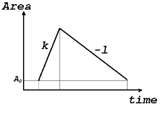
Figure 4: Schematic of time evolution of a sunspot’s area. Here $A_{0}$ is the area of the spot at the time when it first emerges through the photosphere.

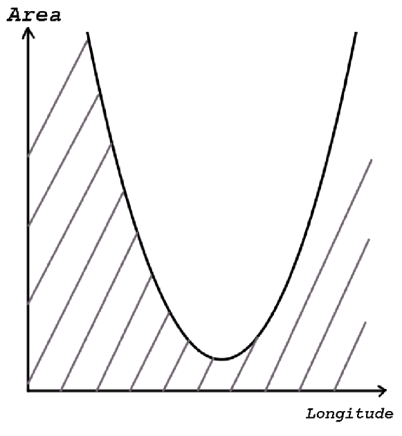
Figure 5: Schematic of Minnaert’s graphical representation (adapted from Minnnaert 1939). The black curve is the visibility function $s(\lambda)$ and the grey parallel curves represent the growth curves of sunspot regions.

The combination of region evolution and rotation, together with the specific form of the visibility function, determines whether a sunspot region is seen or not, and the location and time of its first appearance (and of its disappearance) to an Earth observer. This is clear from Minnaert’s graphical representation (Minnaert 1939), as shown in Fig. 5. The curve in the diagram represents the visibility function $s(\lambda)$, giving the actual area that a sunspot region needs to reach to be visible at longitude $\lambda$. The parallel lines at a slope represent growth phases of sunspots. When a sunspot region growing along a given line crosses $s(\lambda)$, it becomes visible. From this graphical representation it can be seen that if the visibility function has a strong centre-to-limb variation, many spots forming in the west are invisible. An east-west asymmetry in the number of regions observed emerging thus results, and the asymmetry depends on the gradient $s^{\prime}$ of the visibility function.

The process qualitatively represented by Minnaert’s graph was quantitatively described by Schuster (1911), as follows. Let $\lambda_{1}$ indicate the longitude at which a sunspot forms, and $\lambda$ the longitude at which it is first seen because it has crossed the visibility curve $s(\lambda)$. The two longitudes are related by the following equation:

$$A_{0}+k\,\,\frac{\lambda-\lambda_{1}}{\Omega}=s(\lambda)$$ (3)

where $A_{0}$ is the area of the spot when it first emerges, $k$ is the slope of the growth phase and $\Omega$ the solar rotation rate. Eq. 3 expresses the fact that the area at the location where the spot is first seen is equal to $s(\lambda)$.

Eq. 3 can be re-arranged to give:

$$\lambda-\frac{\Omega}{k}\,s(\lambda)=\lambda_{1}-\frac{\Omega}{k}\,A_{0}$$ (4)

which, differentiated, gives:

$$d\lambda\left[1-\frac{\Omega}{k}\,s^{\prime}(\lambda)\right]=d\lambda_{1}$$ (5)

If $N_{1}$ indicates the number of sunspots emerging in a unit longitude bin and $N(\lambda)$ the number of regions observed emerging in a unit bin at longitude $\lambda$, then $N_{1}\,d\lambda_{1}$=$N(\lambda)\,d\lambda$, which gives, using Eq. 5:

$$N(\lambda)=N_{1}\,\left[1-\frac{\Omega}{k}\,s^{\prime}(\lambda)\right]$$ (6)

(Schuster 1911) (Eq (1) of our paper).

Applying the same derivation to the decay phase, characterised by a slope $-$$l$, we obtained Eq. (2) of our paper.

References

- Bogdan et al. (1988) Bogdan T.J., Gilman P.A., Lerche I., and Howard R., Astrophys. J., 327, 451 (1988)
- Dalla et al. (2007) Dalla S., Fletcher L., and Walton N.A., Astron. Astrophys. 468, 1103 (2007)
- Fisher et al. (2000) Fisher G.H., Fan Y., Longcope D.W., Linton M.G.,and Pevtsov A.A., Solar Phys. 192, 119 (2000)
- Foukal et al. (2006) Foukal P., Frolich C., Spruit H. & Wigley T.M., Nature 443, 161 (2006)
- Gallagher et al. (2007) Gallagher P.T., McAteer R.T.J., Young C.A., Ireland J., Hewett R.J. and Conlon P., Solar Activity Monitoring, in Space Weather (ed Lilensten), Astrophysics and Space Science library, Vol. 344, p. 15, Springer (2007)
- Gyori et al. (2004) Gyori L., Baranyi T., Turmon M., and Pap J.M., Adv. Space Res. 34, 269 (2004)
- Harvey (1993) Harvey K.L., Magnetic bipoles on the Sun, PhD thesis, University of Utrecht (1993)
- Howard (1991) Howard R.F., Solar Phys. 134, 233 (1991)
- Hoyt et al. (1983) Hoyt D.V., Eddy J.A., and Hudson H.S., Astrophys. J. 275, 878 (1983)
- Lawrence et al. (1993) Lawrence J.K., K.P. Topka and H.P. Jones, J. Geophys. Res. 98, 18911 (1993)
- Martinez Pillet et al. (1993) Martinez Pillet V., Moreno-Insertis F., and Vazquez M., Astron. Astrophys. 274, 521 (1993)
- Maunder (1907) Maunder A.S.D., Mon. Not. R. Astron. Soc. 67, 451 (1907)
- Minnaert (1939) Minnaert M., Astron. Nachr. 269, 48 (1939) [An English translation is available at: http://www.star.uclan.ac.uk/∼sdalla/minnaert1939.pdf]
- Petrovay & Van Driel-Gesztelyi (1997) Petrovay K. and Van Driel-Gesztelyi L., Solar Phys. 176, 249 (1997)
- Schuster (1911) Schuster A., Proc. Royal Soc. London A 85, 309 (1911)
- Solanki (2003) Solanki S.K., Astron. Astrophys. Rev. 11, 153 (2003)
- Walton et al. (2006) Walton, N.A., Gonzalez-Solarez E., Dalla S., Richards A. & Tedds J., Astron.& Geophys. 47, 3.22 (2006)