Analysis of Lyapunov Method for Control of Quantum States

Abstract

We present a detailed analysis of the convergence properties of Lyapunov control for finite-dimensional quantum systems based on the application of the LaSalle invariance principle and stability analysis from dynamical systems and control theory. Under an ideal choice of the Hamiltonian, convergence results are derived, with a further discussion of the effectiveness of the method when the ideal condition of the Hamiltonian is relaxed.

I Introduction

Control theory has developed into a very broad and interdisciplinary subject. One of its major concerns is how to design the dynamics of a given system to steer it to a desired target state, and how to stabilize the system in a desired state. Assuming that the evolution of the controlled system is described by a differential equation, many control methods have been proposed, including optimal control Lewis ; Kirk , geometric control Jurdjevic97 and feedback control Franklin .

Quantum control theory is about the application of classical and modern control theory to quantum systems. The effective combination of control theory and quantum mechanics is not trivial for several reasons. For classical control, feedback is a key factor in the control design, and there has been a strong emphasis on robust control of linear control systems. Quantum control systems, on the other hand, cannot usually be modelled as linear control systems, except when both the system and the controller are quantum systems and their interaction is fully coherent or quantum-mechanical IEEETAC48p2107 . This is not the case for most applications, where we usually desire to control the dynamics of a quantum system through the interaction with fields produced by what are effectively classical actuators, whether these be control electrodes or laser pulse shaping equipment. Moreover, feedback control for quantum systems is a nontrivial problem as feedback requires measurements, and any observation of a quantum system generally disturbs its state, and often results in a loss of quantum coherence that can reduce the system to mostly classical behavior. Finally, even if measurement backaction can be mitigated, quantum phenomena often take place on sub-nanosecond (in many case femto- or attosecond) timescales and thus require ultrafast control, making real-time feedback unrealistic at present.

This is not to say that measurement-based quantum feedback control is unrealistic. There are various interesting applications, e.g., in the area of laser cooling of atomic motion PRL92n223004 , or for deterministic quantum state reduction PRL96n010504 and stabilization of quantum states, to mention only a few, and progress in technology will undoubtedly lead to new applications. Nonetheless, there are many applications of open-loop Hamiltonian engineering in diverse areas from quantum chemistry to quantum information processing. Even in the area of open-loop control many control design strategies, both geometry jurdjevic1 ; lowenthal ; d'alessandro ; schirmer and optimization-based Shi1988 ; Maday2003 ; schirmer1 , utilize some form of model-based feedback. A particular example is Lyapunov control, where a Lyapunov function is defined and feedback from a model is used to generate controls to minimize its value. Although there have been several papers discussing the application of Lyapunov control to quantum systems, the question of when, i.e., for which systems and objectives, the method is effective and when it is not, has not been answered satisfactorily.

Several early papers on Lyapunov control for quantum systems such as Vettori ; Ferrante ; Grivopoulos considered only control of pure-state systems, and target states that are eigenstates of the free Hamiltonian $H_{0}$, and therefore fixed points of the dynamical system. For target states that are not eigenstates of $H_{0}$, i.e., evolve with time, the control problem can be reformulated either in terms of asymptotic convergence of the system’s actual trajectory to that of the time-dependent target state, or as convergence to the orbit of the target state (or more precisely its closure). Such cases have been discussed in several papers  Mirrahimi2004a ; Mirrahimi2004b ; Mirrahimi2005 ; altafini1 ; altafini2 but except for altafini1 ; altafini2 , the problem was formulated using the Schrodinger equation and state vectors that can only represent a pure state. To give a complete discussion of Lyapunov control, it is desirable to utilize the density operator description as it is suitable for both mixed-state and pure-state systems, and can be generalized to open quantum systems subject to environmental decoherence or measurements, including feedback control. In altafini1 ; altafini2 Lyapunov control for mixed-state quantum systems was considered but the notion of orbit convergence used is rather weak compared to trajectory convergence, the LaSalle invariant set was only shown to contain certain critical points but not fully characterized, and a stability analysis of the critical points was missing, in addition to other issues such as the assumption of periodicity of orbits, etc. Furthermore, while an attempt was made to establish sufficient conditions to guarantee convergence to a target orbit, the effectiveness of the method for realistic system was not considered.

In this paper we address these issues. We consider the problem of steering a quantum system to a target state using Lyapunov feedback as a trajectory tracking problem for a bilinear Hamiltonian control system defined on a complex manifold, where the trajectory of the target state is generally non-periodic, and analyze the effectiveness of the Lyapunov method as a function of the form of the Hamiltonian and the initial value of the target state. In Sec. II the control problem and the Lyapunov function are defined, and some basic issues such as different notions of convergence and reachability of target states are briefly discussed. In Sec. III the controlled quantum dynamics is formulated as an autonomous dynamical system defined on an extended state space, and LaSalle’s invariance principle lasalle is applied to obtain a characterization of the LaSalle invariant set. This characterization shows that even for ideal systems satisfying the strongest possible conditions on the Hamiltonian, the invariant set is generally large, and the invariance principle alone is therefore not sufficient to conclude asymptotic stability of the target state. Noting that the invariant set must contain the critical points of the Lyapunov function we characterize the former in Sec. IV. In Sec. V we give a detailed analysis of the convergence behaviour of the Lyapunov method for finite-dimensional quantum systems under an ideal control Hamiltonian based on the characterization of the LaSalle invariant set and our stability analysis. The discussion is divided into three parts, control of pseudo-pure states, generic mixed states, and other mixed states. The result is for this ideal choice of Hamiltonian Lyapunov control is effective for most (but not all) target states. Finally, in Sec. VI we relax the unrealistic requirements on the Hamiltonian imposed in Sec. V, and show that this leads to a much larger LaSalle invariant set, and significantly diminished effectiveness of Lyapunov control.

II State and trajectory tracking problem for quantum systems

II.1 Quantum states and evolution

According to the basic principles of quantum mechanics the state of an $n$-level quantum system can be represented by an $n\times n$ positive hermitian operator with unit trace, called a density operator $\rho$, and its evolution is determined by the Liouville von-Neumann equation von-Neumann

$$\dot{\rho}(t)=-i\hbar[H,\rho(t)],$$

where $H$ is the system Hamiltonian, denoted by an $n\times n$ Hermitian operator. If we are considering a sub-system that is not closed, i.e., interacts with an external environment, additional terms are required to account for dissipative effects, although in principle, we can always consider the Hamiltonian dynamics on an enlarged Hilbert space, and we shall restrict our discussion here to Hamiltonian systems. We shall say a density operator $\rho$ represents a pure state if it is a rank-one projector, and a mixed state otherwise. We further define the special class of pseudo-pure states, i.e., density operators with two eigenvalues, one of which occurs with multiplicity $1$, the other with multiplicity $n-1$, and generic mixed states, i.e., density operators with $n$ distinct eigenvalues.

II.2 Control Problem

In the following we consider the bilinear Hamiltonian control system

$$\dot{\rho}(t)=-i[H_{0}+f(t)H_{1},\rho(t)],$$ (1)

where $f(t)$ is an admissible real-valued control field and $H_{0}$ and $H_{1}$ are a free evolution and control interaction Hamiltonian, respectively, both of which will be assumed to be time-independent. We have chosen units such that the Planck constant $\hbar=1$ and can be omitted for convenience.

The general control problem is to design a certain control function $f(t)$ such that the system state $\rho(t)$ with $\rho(0)=\rho_{0}$ will converge to the target state $\rho_{d}$. Since the evolution of a Hamiltonian system is unitary, the spectrum of $\rho(t)$ is therefore time-invariant, or equivalently

$$\operatorname{Tr}[\rho^{n}(t)]=\operatorname{Tr}[\rho_{0}^{n}],\quad\forall n\in{{\rm I}\kern-1.60004pt{\rm N}}.$$ (2)

Hence, for the target state $\rho_{d}$ to be reachable, $\rho_{0}$ and $\rho_{d}$ must have the same spectrum, or entropy in physical terms. If $\rho_{0}$ and $\rho_{d}$ do not have the same spectrum, we can still attempt to minimize the distance $\|\rho(t)-\rho_{d}(t)\|$, but it will always be non-zero if we are restricted to Hamiltonian engineering. For the following analysis we shall assume that the initial and the target state of the system have the same spectrum. If this is the case and the system is density-matrix controllable, or pure-state controllable if the initial state of the system is pure or pseudo-pure, then we can conclude that the target state is reachable, although a particular target state may clearly be reachable even if the system is not controllable JPA35p4125 .

Assuming that $\rho_{0}$ and $\rho_{d}$ have the same spectrum, the quantum control problem can be characterized by the spectrum of the target state. If $\rho_{d}$ is pure, the problem is called a pure-state control problem. Analogously, we can define the pseuo-pure-state control and generic-state control. Pure-state control problems are often represented in terms of Hilbert space vectors or wavefunctions $|\psi\rangle$ evolving according to the Schrödinger equation

$$\frac{d}{dt}|\psi(t)\rangle=-i(H_{0}+f(t)H_{1})|\psi(t)\rangle.$$ (3)

For pure states this wavefunction descritpion is equivalent to the density operator description since any rank-one projector $\rho$ can be written as $\rho=|\psi\rangle\langle\psi|$ for some Hilbert space vector $|\psi\rangle$, but it does not generalize to mixed states, and we shall not use this formalism here.

Since the free Hamiltonian $H_{0}$ can usually not be turned off, it is natural to consider non-stationary target states $\rho_{d}$ evolving according to

$$\dot{\rho}_{d}(t)=-i[H_{0},\rho_{d}(t)].$$ (4)

It is easy to see that $\rho_{d}$ is stationary if and only if it commutes with $H_{0}$, $[H_{0},\rho_{d}(0)]=0$. Thus the problem of quantum state control for most target states is more akin to a trajectory tracking problem, where the objective generally is to find a control $f(t)$ such that the trajectory $\rho(t)$ of the initial state $\rho_{0}$ under the controlled evolution asymptotically converges to a target trajectory $\rho_{d}(t)$.

II.3 Trajectory vs Orbit Tracking

It has been argued that the problem of quantum state control should instead be viewed as an orbit tracking problem altafini1 ; altafini2 , i.e., the problem of steering the trajectory $\rho(t)$ towards the orbit of the target state $\rho_{d}$. However, one problem with this approach is that the notion of orbit tracking is relatively weak as the orbit of a quantum state, or more precisely its closure, under free evolution can be rather large, and there are generally infinitely many distinct quantum states whose orbits under free evolution coincide. For example, even for two-level system evolving under the free Hamiltonian $H_{0}=\operatorname{diag}(0,\omega)$ the trajectories of the pure states $|\Psi_{\pm}\rangle=\frac{1}{\sqrt{2}}(|0\rangle\pm|1\rangle)$ are orthogonal, and thus perfectly distinguishable, for all times $t$, $|\Psi_{\pm}(t)\rangle=\frac{1}{\sqrt{2}}(|0\rangle\pm e^{i\omega t}|1\rangle)$, but their orbits are the same, $\mathcal{O}(\Psi_{+})=\{\Psi(t):\Psi(0)=\Psi_{+},t\geq 0\}=\mathcal{O}(\Psi_{-})$.

For the two-level example above, the orbits are always periodic and thus closed, and we can at least say that if the quantums state $\rho(t)$ converges to the periodic orbit $\mathcal{O}(\rho_{d})$ of $\rho_{d}$, then for every state $\rho_{a}\in\mathcal{O}(\rho_{d})$ there exists a sequence of times $\{t_{k}\}$ such that $\|\rho(t_{k})-\rho_{a}\|\to 0$ as $k\to\infty$, but this notion of convergence is much weaker than the notion of trajectory convergence, which requires $\|\rho(t)-\rho_{d}(t)\|\to 0$ as $t\to\infty$, and we shall see that there are cases where it is possible to track the orbit but not a particular trajectory. The notion of orbit tracking is even more problematic for non-periodic orbits, which comprise the vast majority of orbits for systems of Hilbert dimension $n>2$, except for the measure-zero set of Hamiltonians $H_{0}$ with commensurate energy levels, i.e., with transition frequencies that are rational multiples of each other. Of course, we can still ask the question whether the state of the system converges to the closure of the orbit of a target state, but the dimension of this orbit set is generally very large. For instance, the state manifold of pure states for an $n$-dimensional system has (real) dimension $2n-2$, while the closure of the orbit of any state under a generic Hamiltonian $H_{0}$ has dimension $n-1$.

For these reasons, we shall concentrate on quantum state control in the sense of trajectory tracking as this is the strongest notion of convergence and well-defined for arbitrary trajectories.

II.4 Control Design based on Lyapunov Function

A natural design of $f(t)$ is inspired from the conception of Lyapunov function, which is a very important tool in stability analysis for dynamical systems. For an autonomous dynamical system $\dot{x}=f(x)$, a differentiable scalar function $V(x)$, defined on the phase space $\Omega=\{x\}$, is called a Lyapunov function, if:

1. $V(x)$ is continuous and its partial derivatives are also continuous on $\Omega$;

2. $V(x)$ is positive definite, i.e., $V(x)\geq 0$ with equality only at $x=x_{0}$;

3. for any dynamical flow $\phi_{t}(x)$, $\dot{V}(\phi_{t}(x))=\dot{V}(x(t))\leq 0$.

With the conditions above, it can be shown that $x=x_{0}$ is Lyapunov stable; if equality in (iii) holds only for $x=x_{0}$, we can further conclude that $x=x_{0}$ is asymptotically stable. However, in general, we can only guarantee $\dot{V}\leq 0$, and in this case, we can only use a weaker result known as the LaSalle invariance principle lasalle , which claims that any bounded solution will converge to an invariant set, called the LaSalle invariant set.

Let $\mathcal{M}$ to be the set of density operators isospectral with $\rho_{d}(0)$ and consider the joint dynamics for $(\rho(t),\rho_{d}(t))$ on $\mathcal{M}\times\mathcal{M}$:

$$\dot{\rho}(t) =-i[H_{0}+f(t)H_{1},\rho(t)],$$ (5a)

$$\dot{\rho}_{d}(t) =-i[H_{0},\rho_{d}(t)].$$ (5b)

The Hilbert-Schmidt norm $\|A\|=\sqrt{\operatorname{Tr}(A^{\dagger}A)}$ induces a natural distance function on $\mathcal{M}\times\mathcal{M}$, which provides a natural candidate for a Lyapunov function

$$V(\rho,\rho_{d})=\frac{1}{2}\|\rho-\rho_{d}\|^{2}=\frac{1}{2}\operatorname{Tr}[(\rho-\rho_{d})^{2}].$$ (6)

If $\rho$ and $\rho_{d}$ are isospectral, this definition is equivalent to

$$V(\rho,\rho_{d})=\operatorname{Tr}[\rho_{d}^{2}(t)]-\operatorname{Tr}[\rho(t)\rho_{d}(t)],$$ (7)

the Lyapunov function used in altafini1 ; altafini2 . If $\rho_{d}=|\psi_{d}\rangle\langle\psi_{d}|$ and $\rho=|\psi\rangle\langle\psi|$ we have furthermore

$$V(\psi,\psi_{d})=1-|\langle\psi_{d}(t)|\psi(t)\rangle|^{2},$$ (8)

a Lyapunov function often used for pure-state control.

To see that Eq. (7) defines indeed a Lyapunov function, note that $V\geq 0$ with equality only if $\rho=\rho_{d}$, and

$${\dot{V}} =-\operatorname{Tr}(\dot{\rho}_{d}\rho)-\operatorname{Tr}(\rho_{d}\dot{\rho})$$

$$=-\operatorname{Tr}([-iH_{0},\rho_{d}]\rho)-\operatorname{Tr}(\rho_{d}[-iH_{0},\rho])$$

$$\qquad-f(t)\operatorname{Tr}(\rho_{d}[-iH_{1},\rho])$$

$$=-f(t)\operatorname{Tr}(\rho_{d}[-iH_{1},\rho]),$$

where we have used

$$\operatorname{Tr}([-iH_{0},\rho_{d}]\rho)=-\operatorname{Tr}(\rho_{d}[-iH_{0},\rho])$$

and $\frac{d}{dt}\operatorname{Tr}(\rho^{2}_{d})=0$. If we choose the control field as

$$f(\rho,\rho_{d})=\kappa\operatorname{Tr}(\rho_{d}[-iH_{1},\rho]),\quad\kappa>0,$$ (9)

then $\dot{V}(\rho(t),\rho_{d}(t))\leq 0$. Without loss of generality, we set $\kappa=1$ in the following.

Hence, the evolution of the system $(\rho,\rho_{d})$ with Lyapunov feedback is described by the following nonlinear autonomous dynamical system on $\mathcal{M}\times\mathcal{M}$:

$$\dot{\rho(t)} =-i[H_{0}+f(\rho,\rho_{d})H_{1},\rho(t)],$$ (10a)

$$\dot{\rho_{d}(t)} =-i[H_{0},\rho_{d}(t)],$$ (10b)

$$f(\rho,\rho_{d}) =\operatorname{Tr}([-iH_{1},\rho]\rho_{d}).$$ (10c)

The manifold $\mathcal{M}$ here is a homogeneous space known as a flag manifold, whose dimension and topology depend on the spectrum, or more precisely, the number of distinct eigenvalues, of the density operators $\rho$, $\rho_{d}$, under consideration. For pure or pseudo-pure initial states $\rho_{0}$, for example, $\mathcal{M}$ is homeomorphic to the complex projective space ${\rm C\kern-4.49997pt\vrule width=0.29999pt,height=6.24301pt,depth=-0.51663pt\kern 5.0pt}P^{n-1}$, while for a generic mixed state, we obtain the $n^{2}-n$ dimensional manifold $U(n)/\oplus_{\ell=1}^{n}U(1)$. By simply comparing the dimensions, we see that in the special case $n=2$ (and only $2$) the generic mixed states and pseudo-pure states have the same dimension, and one can easily show that in this case all mixed states (except the completely mixed state) are pseudo-pure, a fact that will be relevant later.

III LaSalle Invariance Principle and LaSalle Invariant Set

III.1 Invariance Principle for Autonomous Systems

For an autonomous dynamical system with $\dot{x}=f(x)$, we say a set is invariant, if any flow starting at a point in the set will stay in it for all times. For any solution $x(t)$ we define the positive limiting set $\Gamma^{+}$ to be the set of all limit points of $x(t)$ as $t\to+\infty$. First of all, we have the following two lemmas:

Lemma III.1.

For $\dot{x}=f(x)$ defined on a finite-dimensional manifold, the positive limiting set $\Gamma^{+}$ of any bounded solution $x(t)$ is an non-empty, connected, compact, invariant set.

The proof can be found in Perko (Sec. 3.2, Theorem $2$).

Lemma III.2.

Any bounded solution $x(t)$ will tend to any set containing its positive limiting set $\Gamma^{+}$ as $t\to\infty$.

Proof.

Suppose $x(t)$ does not converge to $\Gamma^{+}$. Then there exists some $\epsilon>0$, and a sequence $t_{n}$ such that $x(t_{n})$ is outside the $\epsilon$-neighborhood of $\Gamma^{+}$. But $x(t_{n})$ is a bounded set, so it has a subsequence that converges to a point $x_{0}$. By assumption $x_{0}\not\in\Gamma^{+}$, which contradicts the definition of the positive limiting set. Hence, $x_{0}$ must belong to the positive limiting set. ∎

From these results we can derive the LaSalle invariance principle lasalle :

Theorem III.1.

For an autonomous dynamical system, $\dot{x}=f(x)$, let $V(x)$ be a Lyapunov function on the phase space $\Omega=\{x\}$, satisfying $V(x)>0$ for all $x\neq x_{0}$ and $\dot{V}(x)\leq 0$, and let $\mathcal{O}(x(t))$ be the orbit of $x(t)$ in the phase space. Then the invariant set $E=\{\mathcal{O}(x(t))|\dot{V}(x(t))=0\}$ contains the positive limiting sets of all bounded solutions, i.e., any bounded solution converges to $E$ as $t\to+\infty$.

Proof.

Since $V(x(t))$ is monotonically decreasing due to $\dot{V}\leq 0$, $V(x(t))$ has a limit $V_{0}\geq 0$ as $t\to+\infty$ for any bounded solution $x(t)$. Let $\Gamma^{+}$ be the positive limiting set of $x(t)$. By continuity, the value of $V$ on $\Gamma^{+}$ must be $V_{0}$. Since $\Gamma^{+}$ is an invariant set, we can take the time derivative of $V$ to conclude $\dot{V}=0$ on $\Gamma^{+}$. By Lemma III.2, $x(t)$ will converge to $\Gamma^{+}$, and hence to $E$. ∎

Remark III.1.

From the proof above, we can see that the theorem holds for both real and complex dynamical systems. Broadly speaking, what has been proved is that bounded solutions with $\dot{V}(x)\neq 0$ will converge to the set of solutions with $\dot{V}(x)=0$. Therefore, it does not matter if $V$ has many points $x$ with $V(x)=0$. For example, for the quantum system (10), the Lyapunov function $V$ is zero on all points $(\rho_{d},\rho_{d})$.

The quantum system (10) is autonomous and defined on the phase space $\mathcal{M}\times\mathcal{M}$, where $\mathcal{M}$ is a compact finite dimensional manifold. Therefore, any solution $(\rho(t),\rho_{d}(t))$ is bounded. Although the Lyapunov function (7) is not positive definite, we have $V=0$ if and only if $\rho=\rho_{d}$, which is sufficient to apply the LaSalle invariance principle III.1 to obtain:

Theorem III.2.

Any system evolution $(\rho(t),\rho_{d}(t))$ under the Lyapunov control (9) will converge to the invariant set $E=\{(\rho_{1},\rho_{2})\in\mathcal{M}\times\mathcal{M}|\dot{V}(\rho(t),\rho_{d}(t))=0,(\rho(0),\rho_{d}(0))=(\rho_{1},\rho_{2})\}$.

We note here that except when $\rho_{d}$ is a stationary state, we must consider the dynamical system on the extended phase space $\mathcal{M}\times\mathcal{M}$ as $V$ is not well-defined on $\mathcal{M}$. Having established convergence to the LaSalle invariant set $E$, the next step is to characterize $E$ for the dynamical system (10).

III.2 Characterization of the LaSalle Invariant Set

LaSalle’s invariance principle reduces the convergence analysis to calculating the invariant set $E=\{\dot{V}(\rho(t),\rho_{d}(t))=0\}$, which is equivalent to $f(t)=0$, for any $t$. Therefore, we have

$$0 =f=\operatorname{Tr}([-iH_{1},\rho]\rho_{d})$$

$$0 =\dot{f}=\operatorname{Tr}([-iH_{1},\rho]\dot{\rho}_{d})+\operatorname{Tr}([-iH_{1},\dot{\rho}]\rho_{d})$$

$$\qquad-\operatorname{Tr}([[-iH_{0},-iH_{1}],\rho]\rho_{d})$$

$$\cdots$$

$$0 =\frac{d^{\ell}f}{dt^{\ell}}=(-1)^{n}\operatorname{Tr}([\operatorname{Ad}^{\ell}_{-iH_{0}}(-iH_{1}),\rho]\rho_{d}),$$

where $\operatorname{Ad}^{\ell}_{-iH_{0}}(-iH_{1})$ represents $\ell$-fold commutator adjoint action of $-iH_{0}$ on $-iH_{1}$. Hence, $\operatorname{Tr}([A,B]C)=-\operatorname{Tr}([C,B]A)=-\operatorname{Tr}([A,C]B)$ gives a necessary condition for the invariant set $E$:

$$\operatorname{Tr}([\rho,\rho_{d}]\operatorname{Ad}^{m}_{-iH_{0}}(-iH_{1}))=0,\qquad\forall m\in{{\rm I}\kern-1.60004pt{\rm N}}_{0},$$ (11)

where $\operatorname{Ad}^{0}_{-iH_{0}}(-iH_{1})=-iH_{1}$. Since $H_{0}$ is Hermitian we can choose a basis such that $H_{0}$ is diagonal

$$H_{0}=\begin{pmatrix}a_{1}&0&\ldots&0\\ 0&a_{2}&\ldots&0\\ \vdots&&\ddots&\vdots\\ 0&0&\ldots&a_{n}\end{pmatrix}\equiv\operatorname{diag}(a_{1},\ldots,a_{n})$$

with real eigenvalues $a_{k}$, which we may assume to be arranged so that $a_{k}\geq a_{k+1}$ for all $k$. Let $(b_{k\ell})$ be the matrix representation of $H_{1}$ in the eigenbasis of $H_{0}$, and $\omega_{k\ell}=a_{\ell}-a_{k}$ be the transition frequency between energy levels $k$ and $\ell$ of the system.

The Lie algebra $\mathfrak{su}(n)$ can be decomposed into an abelian part called the Cartan subalgebra $\mathcal{C}=\operatorname{span}\{\lambda_{k}\}_{k=1}^{n-1}$, and an orthogonal subalgebra $\mathcal{T}$, which is a direct sum of $n(n-1)/2$ root spaces spanned by pairs of generators $\{\lambda_{k\ell},\bar{\lambda}_{k\ell}\}$. For instance, we can choose the generators

$$\lambda_{k} =i(\hat{e}_{kk}-\hat{e}_{k+1,k+1})$$ (12a)

$$\lambda_{k\ell} =i(\hat{e}_{k\ell}+\hat{e}_{\ell k})$$ (12b)

$$\bar{\lambda}_{k\ell} =(\hat{e}_{k\ell}-\hat{e}_{\ell k})$$ (12c)

for $1\leq k<\ell\leq n$, where the $(k,\ell)^{\rm th}$ entry of the elementary matrix $\hat{e}_{mn}$ equals $\delta_{km}\delta_{\ell n}$. Expanding $-iH_{1}\in\mathfrak{su}(n)$ with respect to these generators

$$-iH_{1}=\sum_{k=1}^{n-1}\left[b_{k}\lambda_{k}+\sum_{\ell=k+1}^{n}-\Re(b_{k\ell})\lambda_{k\ell}+\Im(b_{k\ell})\bar{\lambda}_{k\ell}\right]$$ (13)

and noting that we have for $D=\sum_{k=1}^{n}d_{k}\hat{e}_{kk}$

$$[D,\lambda_{k}] =0,$$ (14a)

$$[D,\lambda_{k\ell}] =+i(d_{k}-d_{\ell})\bar{\lambda}_{k\ell},$$ (14b)

$$[D,\bar{\lambda}_{k\ell}] =-i(d_{k}-d_{\ell})\lambda_{k\ell},$$ (14c)

shows that $B_{m}=\operatorname{Ad}_{-iH_{0}}^{m}(-iH_{1})$ is equal to

$$B_{2m-1} =\sum_{k=1}^{n-1}\sum_{\ell=k+1}^{n}\!\!\!(-1)^{m}\omega_{k\ell}^{2m-1}[\Re(b_{k\ell})\bar{\lambda}_{k\ell}+\Im(b_{k\ell})\lambda_{k\ell}],$$ (15a)

$$B_{2m} =\sum_{k=1}^{n-1}\sum_{\ell=k+1}^{n}(-1)^{m}\omega_{k\ell}^{2m}[\Re(b_{k\ell})\lambda_{k\ell}-\Im(b_{k\ell})\bar{\lambda}_{k\ell}].$$ (15b)

Let$\mathcal{B}^{s}=\operatorname{span}\{B_{m}\}_{m=1}^{s}$ and $\mathcal{B}_{0}^{s}=\operatorname{span}\{B_{m}\}_{m=0}^{s}$ with $B_{0}=-iH_{1}$. Then Eq (11) is equivalent to $[\rho,\rho_{d}]$ being orthogonal to the subspace $\mathcal{B}_{0}^{s}$ with respect to the Hilbert-Schmidt norm.

Theorem III.3.

The subspace $\mathcal{B}^{n^{2}-n}$ generated by the Ad-brackets is a subset of the Cartan subalgebra $\mathcal{T}$ of $\mathfrak{su}(n)$ with equality if

• $H_{0}$ is strongly regular, i.e., $\omega_{k\ell}\neq\omega_{pq}$ unless $(k,\ell)=(p,q)$.

• $H_{1}$ is fully connected, i.e., $b_{k\ell}\neq 0$ except (possibly) for $k=\ell$.

Proof.

Since the dimension of $\mathcal{T}$ is $n^{2}-n$ and $B_{m}\in\mathcal{T}$ for all $m>0$, it suffices to show that the elements $B_{m}$ for $m=1,\ldots,n^{2}-n$ are linearly independent. Moreover, the subspaces spanned by the odd and even order elements, $\mathcal{B}_{\rm odd}^{s}=\operatorname{span}\{B_{2m-1}:1\leq 2m-1\leq s\}$ and $\mathcal{B}_{\rm even}^{s}=\operatorname{span}\{B_{2m}:1\leq 2m\leq s\}$, respectively, are orthogonal since

$$B_{2m-1}B_{2m^{\prime}}=(-1)^{m+m^{\prime}}\sum_{k,\ell}\sum_{k^{\prime},\ell^{\prime}}\omega_{k\ell}^{2m-1}\omega_{k^{\prime}\ell^{\prime}}^{2m^{\prime}}\times\\ [\Re(b_{k\ell})\Re(b_{k^{\prime}\ell^{\prime}})\bar{\lambda}_{k\ell}\lambda_{k^{\prime}\ell^{\prime}}-\Im(b_{k\ell})\Im(b_{k^{\prime}\ell^{\prime}})\lambda_{k\ell}\bar{\lambda}_{k^{\prime}\ell^{\prime}}\\ -\Re(b_{k\ell})\Im(b_{k^{\prime}\ell^{\prime}})\bar{\lambda}_{k\ell}\bar{\lambda}_{k^{\prime}\ell^{\prime}}+\Im(b_{k\ell})\Re(b_{k^{\prime}\ell^{\prime}})\lambda_{k\ell}\lambda_{k^{\prime}\ell^{\prime}}],$$

and thus observing the equalities

$$\operatorname{Tr}(\lambda_{k\ell}\lambda_{k^{\prime}\ell^{\prime}})=\operatorname{Tr}(\bar{\lambda}_{k\ell}\bar{\lambda}_{k^{\prime}\ell^{\prime}})=-2\delta_{kk^{\prime}}\delta_{\ell\ell^{\prime}}$$ (16a)

$$\operatorname{Tr}(\lambda_{k\ell}\bar{\lambda}_{k^{\prime}\ell^{\prime}})=0$$ (16b)

shows that for all $m,m^{\prime}>0$

$$\operatorname{Tr}(B_{2m-1}B_{2m^{\prime}})=(-1)^{m+m^{\prime}}\sum_{k,\ell}\sum_{k^{\prime},\ell^{\prime}}\omega_{k\ell}^{2m-1}\omega_{k^{\prime}\ell^{\prime}}^{2m^{\prime}}\times\\ \Re(b_{k\ell})\Im(b_{k\ell})[-\bar{\lambda}_{k\ell}^{2}+\lambda_{k\ell}^{2}]=0.$$

Thus it suffices to show that the elements of $\mathcal{B}_{\rm odd}^{n^{2}-n}$ and $\mathcal{B}_{\rm even}^{n^{2}-n}$ are linearly independent separately.

For the odd terms, suppose there exists a vector $\vec{c}=(c_{1},\ldots,c_{s})^{T}$ of length $s=n(n-1)/2$ such that $\sum_{m=1}^{s}c_{m}B_{2m-1}=0$. Noting that $\omega_{kk}=0$ and $(\omega_{\ell k})^{2}=(-\omega_{k\ell})^{2}$ this gives $n(n-1)/2$ non-trivial equations

$$\omega_{k\ell}[\Re(b_{k\ell})\bar{\lambda}_{k\ell}+\Im(b_{k\ell})\lambda_{k\ell}]\;\sum_{m=1}^{s}(-\omega_{k\ell}^{2})^{m-1}c_{m}=0,$$ (17)

for $1\leq k<\ell\leq n$. Since $\omega_{k\ell}\neq 0$, $b_{k\ell}\neq 0$ by hypothesis, Eq. (17) can be reduced to $\Omega\vec{c}=\vec{0}$, where $\Omega$ is a matrix:

$$\Omega=\begin{pmatrix}1&-\omega_{12}^{2}&\omega_{12}^{4}&\ldots&(-\omega_{12}^{2})^{m-1}\\ 1&-\omega_{13}^{2}&\omega_{13}^{4}&\ldots&(-\omega_{13}^{2})^{m-1}\\ \vdots&\vdots&\vdots&\ddots&\vdots\\ 1&-\omega_{n-1,n}^{2}&\omega_{n-1,n}^{4}&\ldots&(-\omega_{n-1,n}^{2})^{m-1}\\ \end{pmatrix}.$$ (18)

Since $\Omega$ is a Vandermonde matrix, condition (ii) of the proposition guarantees that Eq. (17) has only the trivial solution $\vec{c}=\vec{0}$, thus establishing linear independence. For the even terms we obtain a similar system of equations, which completes the proof. ∎

If $\mathcal{B}^{n^{2}-n}=\mathcal{T}$ then any point $(\rho_{1},\rho_{2})$ in the invariant set $E$ must satisfy $[\rho_{1},\rho_{2}]=\operatorname{diag}(c_{1},\ldots,c_{n})$. Furthermore, $\operatorname{Tr}(-iH_{1}[\rho_{1},\rho_{2}])=0$ yields in addition

$$-i\sum_{k,\ell=1}^{n}b_{k\ell}c_{\ell k}=-i\sum_{k=1}^{n}b_{kk}c_{kk}=0.$$ (19)

However, in many applications the energy level shifts induced by the field are negligible, and we can assume the diagonal elements of $H_{1}$ to be zero. With this additional assumption we have $\mathcal{B}_{0}^{s}\subset\mathcal{T}$, and thus the maximum dimension of $\mathcal{B}_{0}^{s}$ is $n^{2}-n$, and we have the following useful result.

Theorem III.4.

Under conditions (i) and (ii) of Theorem III.3 $(\rho_{1},\rho_{2})$ belongs to the invariant set $E$ if and only if $[\rho_{1},\rho_{2}]=\operatorname{diag}(c_{1},\ldots,c_{n})$.

Proof.

We have proved the necessary part. For the sufficient part note that $\rho_{k}(t)=e^{-iH_{0}t}\rho_{k}e^{iH_{0}t}$, $k=1,2$,

$$[e^{-iH_{0}t}\rho_{1}e^{iH_{0}t},e^{-iH_{0}t}\rho_{2}e^{iH_{0}t}]=e^{-iH_{0}t}[\rho_{1},\rho_{2}]e^{iH_{0}t}$$

and $e^{-iH_{0}t}$ diagonal. Thus if $[\rho_{1},\rho_{2}]=\operatorname{diag}(c_{1},\ldots,c_{n})$ then $e^{-iH_{0}t}[\rho_{1},\rho_{2}]e^{iH_{0}t}=\operatorname{diag}(c_{1},\ldots,c_{n})=[\rho_{1},\rho_{2}]$ and hence $(\rho_{1},\rho_{2})\in E$. ∎

Thus we have fully characterized the invariant set for systems with strongly regularly $H_{0}$ and an interaction Hamiltonian $H_{1}$ with a fully connected transition graph. The result also shows that even under the most stringent assumptions about the system Hamiltonians, the invariant set is generally much larger than the desired solution. Therefore, the invariance principle alone is not sufficient to establish convergence to the target state.

IV Critical Points of the Lyapunov Function

In this section we show that invariant set $E$ always contains at least the critical points of the Lyapunov function $V$ and classify the stability of the critical points. We start with the case where $\rho_{d}$ is a fixed stationary state. In this case the Lyapunov function $V(\rho,\rho_{d})$ is effectively a function $V(\rho)$ on $\mathcal{M}$. Since $\rho$ can be written as $\rho=U\rho_{d}U^{\dagger}$ for some $U$ in the special unitary group $\mathfrak{SU}(n)$, $V$ also be considered a function on $\mathfrak{SU}(n)$, $V(U)=V(U\rho_{d}U^{\dagger}\rho_{d})$. It is easy to see that the critical points of $V(\rho)$ correspond to those of $V(U)$, and since $\operatorname{Tr}[\rho_{d}(t)]^{2}=C$ is constant, it is equivalent to find the critical points of $J(U)$:

$$J(U) =C-V(U)$$

$$=\operatorname{Tr}(U\rho_{d}U^{\dagger}\rho_{d}),\quad U\in\mathfrak{SU}(n).$$ (20)

Lemma IV.1.

The critical points $U_{0}$ of $J(U)$ defined by (IV) are such that $[\rho_{0},\rho_{d}]=0$ for $\rho_{0}=U_{0}\rho_{d}U_{0}^{\dagger}$.

Proof.

Let $\{\sigma_{m}\}_{m=1}^{n^{2}-1}$ be an orthonormal basis for the Lie algebra $\mathfrak{su}(n)$, consisting of $n^{2}-n$ orthonormal off-diagonal generators such as $\frac{1}{\sqrt{2}}\lambda_{k\ell}$, $\frac{1}{\sqrt{2}}\bar{\lambda}_{k\ell}$ with $\lambda_{k\ell},\bar{\lambda}_{k\ell}$ as in Eq. (12), and $n-1$ orthonormal diagonal generators

$$\sigma_{n^{2}-n+r}=\frac{i}{\sqrt{r(r+1)}}\left(\sum_{s=1}^{r}\hat{e}_{ss}-r\hat{e}_{r+1,r+1}\right)$$ (21)

for $r=1,\ldots,n-1$. Set $\vec{\sigma}=(\sigma_{1},\ldots,\sigma_{n^{2}-1})$. Any $U\in\mathfrak{SU}(n)$ near the identity $I$ can be written as $U=e^{\vec{x}\cdot\vec{\sigma}}$, where $\vec{x}\in{{\rm I}\kern-1.60004pt{\rm R}}^{n}$ is the coordinate of $U$, and any $U$ in the neighborhood of $U_{0}$ can be parameterized as $U=e^{\vec{x}\cdot\vec{\sigma}}U_{0}$. Thus Eq. (IV) becomes

$$J=\operatorname{Tr}[(e^{\vec{x}\cdot\vec{\sigma}}U_{0})\rho_{d}(U_{0}^{\dagger}e^{-\vec{x}\cdot\vec{\sigma}})\rho_{d}].$$ (22)

At the critical point $U_{0}$, $\nabla J=0$ implies that for all $m$

$$0=\frac{\partial J}{\partial x_{m}} =\operatorname{Tr}(\sigma_{m}U_{0}\rho_{d}U_{0}^{\dagger}\rho_{d}-U_{0}\rho_{d}U_{0}^{\dagger}\sigma_{m}\rho_{d})$$

$$=\operatorname{Tr}[\sigma_{m}(U_{0}\rho_{d}U_{0}^{\dagger}\rho_{d}-\rho_{d}U_{0}\rho_{d}U_{0}^{\dagger})]$$

$$=\operatorname{Tr}(\sigma_{m}[U_{0}\rho_{d}U_{0}^{\dagger},\rho_{d}]).$$ (23)

Thus $[U_{0}\rho_{d}U_{0}^{\dagger},\rho_{d}]\in\mathfrak{su}(n)$ is orthogonal to all basis elements $\sigma_{m}$, and therefore $[U_{0}\rho_{d}U_{0}^{\dagger},\rho_{d}]=0$. ∎

Hence, for a given $\rho_{d}$, the critical points of $V(\rho)$ are such that $[\rho,\rho_{d}]=0$, i.e., $\rho$ and $\rho_{d}$ are simultaneously diagonalizable. Let $\{w_{1},\ldots,w_{n}\}$ be the spectrum of $\rho_{d}$ with $w_{k}$ arranged in a non-increasing order. For any critical point $\rho_{0}$ there thus exists a basis such that

$$\rho_{d} =\operatorname{diag}(w_{1},\ldots,w_{n}),$$

$$\rho_{0} =\operatorname{diag}(w_{\tau(1)},\ldots,w_{\tau(n)}),$$

for some permutation $\tau$ of the numbers $\{1,\ldots,n\}$, and the corresponding critical value of $V$ is

$$V(\rho_{0},\rho_{d})=\sum_{k=1}^{n}w_{k}(w_{k}-w_{\tau(k)}).$$ (24)

More generally, for $V(\rho_{1},\rho_{2})$ defined on $\mathcal{M}\times\mathcal{M}$, there exists $U_{1}$ and $U_{2}$ such that

$$\rho_{1}=U_{1}\rho_{d}U_{1}^{\dagger},\quad\rho_{2}=U_{2}\rho_{d}U_{2}^{\dagger}.$$

Since $\operatorname{Tr}(\rho_{2}^{2})$ is constant, the critical points of $V$ are again the critical points of $J(\rho_{1},\rho_{2})=\operatorname{Tr}(\rho_{1}\rho_{2})$ and

$$J(U_{1},U_{2}) =\operatorname{Tr}\Big{(}U_{1}\rho_{d}U_{1}^{\dagger}U_{2}\rho_{d}U_{2}^{\dagger}\Big{)}$$

$$=\operatorname{Tr}\Big{(}(U_{2}^{\dagger}U_{1})\rho_{d}(U_{2}^{\dagger}U_{1})^{\dagger}\rho_{d}\Big{)}$$

together with Lemma IV.1 shows that $J$ attains its critical value when $[(U_{2}^{\dagger}U_{1})\rho_{d}(U_{2}^{\dagger}U_{1})^{\dagger},\rho_{d}]=0$, and thus

$$0 =U_{2}[(U_{2}^{\dagger}U_{1})\rho_{d}(U_{2}^{\dagger}U_{1})^{\dagger},\rho_{d}]U_{2}^{\dagger}$$

$$=[U_{1}\rho_{d}U_{1}^{\dagger},U_{2}\rho_{d}U_{2}^{\dagger}]=[\rho_{1},\rho_{2}].$$

Thus we have the following:

Theorem IV.1.

For a given $\rho_{d}$, the critical points of the Lyapunov function $V(\rho_{1},\rho_{2})$ on $\mathcal{M}\times\mathcal{M}$ are such that $\{[\rho_{1},\rho_{2}]=0\}$. Therefore, the LaSalle invariant set contains all the critical points of $V(\rho_{1},\rho_{2})$.

Next, we show that for a generic stationary state $\rho_{d}$, $J(\rho)=\operatorname{Tr}(\rho\rho_{d})$, and thus $V(\rho)=V(\rho,\rho_{d})$, is a Morse function Morse on $\mathcal{M}$, i.e., its critical points are hyperbolic:

Theorem IV.2.

If $\rho_{d}$ has non-degenerate eigenvalues then $J(\rho)$ is a Morse function on $\mathcal{M}$. Moreover, all but two critical points corresponding to the global maximum and minimum of $J$, respectively, are saddle points with critical values $J_{0}$ satisfying $J_{\rm min}<J_{0}<J_{\rm max}$.

Proof.

For non-degenerate $\rho_{d}$, we choose a basis such that $\rho_{d}=\operatorname{diag}(w_{1},\ldots,w_{n})$ with $w_{k}$ arranged in decreasing order. Then there are $n!$ critical points satisfying $\rho_{0}=\operatorname{diag}(w_{\tau(1)},\ldots,w_{\tau(n)})$, for some permutation $\tau$, corresponding to the critical value $J(\rho_{0})=\sum_{k=1}^{n}w_{k}w_{\tau(k)}$. Again, we consider $J=\operatorname{Tr}(\rho\rho_{d})=\operatorname{Tr}(U\rho_{d}U^{\dagger}\rho_{d})$ as a function on $\mathfrak{SU}(n)$. Let $U_{0}$ correspond to the critical point $\rho_{0}$. As in the proof of Theorem IV.1, any $U$ in the neighborhood of $U_{0}$ can again be parameterized as $U=e^{\vec{x}\cdot\vec{\sigma}}U_{0}$. Substituting this into $J$, we obtain:

$$J =\operatorname{Tr}[e^{\vec{x}\cdot\vec{\sigma}}U_{0}\rho_{d}U_{0}^{\dagger}e^{-\vec{x}\cdot\vec{\sigma}}\rho_{d}]$$

$$=\operatorname{Tr}[(I+\vec{x}\cdot\vec{\sigma}+\frac{1}{2}(\vec{x}\cdot\vec{\sigma})^{2})\times U_{0}\rho_{d}U_{0}^{\dagger}\times$$

$$\qquad(I-\vec{x}\cdot\vec{\sigma}+\frac{1}{2}(\vec{x}\cdot\vec{\sigma})^{2})\rho_{d}]+\Theta(|\vec{x}|^{3})$$

$$=\operatorname{Tr}[U_{0}\rho_{d}U_{0}^{\dagger}\rho_{d}]+\frac{1}{2}\operatorname{Tr}[(\vec{x}\cdot\vec{\sigma})^{2}U_{0}\rho_{d}U_{0}^{\dagger}\rho_{d}]$$

$$\quad+\frac{1}{2}\operatorname{Tr}[U_{0}\rho_{d}U_{0}^{\dagger}(\vec{x}\cdot\vec{\sigma})^{2}\rho_{d}]$$

$$\quad-\operatorname{Tr}[(\vec{x}\cdot\vec{\sigma})U_{0}\rho_{d}U_{0}^{\dagger}(\vec{x}\cdot\vec{\sigma})\rho_{d}]+\Theta(|\vec{x}|^{3})$$

Choosing a curve in $\mathfrak{SU}(n)$ passing through $U_{0}$ such that $\vec{x}\cdot\vec{\sigma}=\lambda_{k\ell}t$, we have

$$J = \operatorname{Tr}[U_{0}\rho_{d}U_{0}^{\dagger}\rho_{d}]+t^{2}\{\operatorname{Tr}(\lambda_{k\ell}U_{0}\rho_{d}U_{0}^{\dagger}\lambda_{k\ell}^{\dagger}\rho_{d})$$

$$-\operatorname{Tr}(U_{0}\rho_{d}U_{0}^{\dagger}\rho_{d})\}+\Theta(|t|^{3}).$$

Analogously, choosing a curve in $SU(n)$ passing through $U_{0}$ such that $\vec{x}\cdot\vec{\sigma}=\bar{\lambda}_{k\ell}t$, we have

$$J = \operatorname{Tr}[U_{0}\rho_{d}U_{0}^{\dagger}\rho_{d}]+t^{2}\{\operatorname{Tr}(\bar{\lambda}_{k\ell}U_{0}\rho_{d}U_{0}^{\dagger}\bar{\lambda}_{k\ell}^{\dagger}\rho_{d})$$

$$-\operatorname{Tr}(U_{0}\rho_{d}U_{0}^{\dagger}\rho_{d})\}+\Theta(|t|^{3}).$$

The conjugate action of $\lambda_{k\ell}$ or $\bar{\lambda}_{k\ell}$ on the critical point $\rho_{0}=U_{0}\rho_{d}U_{0}^{\dagger}$ swaps the $k$-th and $\ell$-th diagonal elements. Since $\rho_{d}$ is non-degenerate, any swap $\lambda_{k\ell}$ or $\bar{\lambda}_{k\ell}$ will either increase or decrease the value of $J=\sum_{k=1}^{n}w_{k}w_{\tau(k)}$, corresponding to a minimum or maximum along that direction. This holds for all directions of $\lambda_{k\ell}$ and $\bar{\lambda}_{k\ell}$, and since the dimensions of $\mathcal{T}$ and $\mathcal{M}$ are both $n^{2}-n$, we have found $n^{2}-n$ independent directions along which $J$ corresponds to a maximum or minimum. Thus these $n!$ critical points are all hyperbolic. The maximal critical value occurs only when $\rho_{0}=\rho_{d}$ and the minimal value occurs only when $w_{\tau(k)}$’s are in an increasing order. For all other critical values, there always exists a swap that will increase the value of $J$ and a swap that will decrease it, showing that they are saddle points of the $J$. ∎

V Lyapunov Control under an ideal Hamiltonian

In this section we consider the implications of the results of the previous sections on the convergence behaviour and effectiveness of Lyapunov control of a quantum system under an ideal Hamiltonian, i.e., assuming $H_{0}$ is strongly regular and $H_{1}$ is off-diagonal and fully connected. Without loss of generality we can also assume $H_{0}\in\mathfrak{su}(n)$, as the identity part of $H_{0}$ only changes the global phase. Once the form of the Hamiltonian is fixed, the LaSalle invariant set $E$ depends on the target state $\rho_{d}$ only. We discuss in detail the two most important cases when (a) $\rho_{d}$ is a pseudo-pure state and hence $\operatorname{dim}(\mathcal{M})=2n-2$, and when (b) $\rho_{d}$ is generic and $\operatorname{dim}(\mathcal{M})=n^{2}-n$, and conclude with a brief discussion of degenerate stationary target states $\rho_{d}$.

V.1 Pseudo-pure state control

In this section we consider the special class of density operators acting on $\mathcal{H}={\rm C\kern-4.49997pt\vrule width=0.29999pt,height=6.24301pt,depth=-0.51663pt\kern 5.0pt}^{n}$ whose spectrum consists of two eigenvalues $\{w,u\}$ where $u=(1-w)/(n-1)$ occurs with multiplicity $n-1$, which includes pure states with spectrum $\{1,0\}$. We first consider the special case of a two-level system as the results for this case can be easily visualized in ${{\rm I}\kern-1.60004pt{\rm R}}^{3}$ and are useful in the general discussion of pure-state control problems for $n$-level systems that follows.

V.1.1 Two-level systems

For a two-level system strong regularity of $H_{0}$ simply means that the energy levels are non-degenerate and full connectivity of $H_{1}$ requires only $b_{12}\neq 0$, conditions that are satisfied in all but trivial cases. The density operator of a two-level system can be written as

$$\rho=\frac{1}{2}\left(\sigma_{0}+x\sigma_{x}+y\sigma_{y}+z\sigma_{z}\right),$$ (25)

where $\vec{s}=(x,y,z)\in{{\rm I}\kern-1.60004pt{\rm R}}^{3}$ and the Pauli matrices are

$$\sigma_{0}=\begin{bmatrix}1&0\\ 0&1\end{bmatrix},\sigma_{x}=\begin{bmatrix}0&1\\ 1&0\end{bmatrix},\sigma_{y}=\begin{bmatrix}0&-i\\ i&0\end{bmatrix},\sigma_{z}=\begin{bmatrix}1&0\\ 0&-1\end{bmatrix}.$$

Noting that $\operatorname{Tr}(\rho^{2})=\frac{1}{2}(1+\|\vec{s}\|^{2})$ shows that in this representation pure states, characterized by $\operatorname{Tr}(\rho^{2})=1$, correspond to points on the surface of the unit sphere $S^{2}\in{{\rm I}\kern-1.60004pt{\rm R}}^{3}$, while mixed states ($\operatorname{Tr}(\rho^{2})<1$) correspond to points in the interior. The vector $\vec{s}$ is often called the Bloch vector of the quantum state. Any unitary evolution of $\rho(t)$ under a constant Hamiltonian corresponds to a rotation of $\vec{s}(t)$ about a fixed axis in ${{\rm I}\kern-1.60004pt{\rm R}}^{3}$, and free evolution under $H_{0}=\operatorname{diag}(a_{1},a_{2})$ in particular corresponds to a rotation of the Bloch vector $\vec{s}(t)$ about the $z$-axis. Thus, in this special case the path $\vec{s}(t)$ traced out by any Bloch vector $\vec{s}_{0}$ evolving under any constant Hamiltonian forms a circle, i.e., a closed periodic orbit.

Let $\vec{s}=(x,y,z)$ and $\vec{s}_{d}=(x_{d},y_{d},z_{d})$ be the Bloch vectors of $\rho$ and $\rho_{d}$, respectively. It is straightforward to show that $[\rho,\rho_{d}]$ diagonal implies

$$zx_{d}-xz_{d}=0,\qquad yz_{d}-zy_{d}=0.$$ (26)

If (a) $z_{d}\neq 0$ then $(x,y)=\alpha(x_{d},y_{d})$ with $\alpha=z/z_{d}$, and thus $x^{2}+y^{2}+z^{2}=\alpha^{2}(x_{d}^{2}+y_{d}^{2}+z_{d}^{2})$, and the RHS has to equal $x_{d}^{2}+y_{d}^{2}+z_{d}^{2}$ since $\|\vec{s}\|=\|\vec{s}_{d}\|$. Thus $\alpha=\pm 1$ and $(x,y,z)=\pm(x_{d},y_{d},z_{d})$, and the corresponding density operators $\rho,\rho_{d}$ commute, $[\rho,\rho_{d}]=0$.

If (b) $z_{d}=0$ then either (b1) $x_{d}=0$ and $y_{d}=0$ or (b2) $z=0$. In case (b1) we have $\vec{s}_{d}=(0,0,0)$, i.e., the target state is the completely mixed state. Since the completely mixed state forms a trivial equivalence class under unitary evolution, the invariant set in this case is $E=\{(\vec{0},\vec{0})\}$. Case (b2) is more interesting with the invariant set being

$$E=\{(\vec{s},\vec{s}_{d}):z=z_{d}=0,x^{2}+y^{2}=x_{d}^{2}+y_{d}^{2}\},$$ (27)

i.e., all pairs of Bloch vectors that lie on a circle of radius $\|\vec{s}_{d}\|$ in the equatorial plane. Notice that this set is significantly larger than the set of critical points of $V$, which consists only of $\{\pm\vec{s}_{d}\}$.

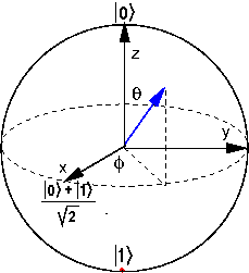
Figure 1: Bloch sphere: There is a one-to-one correspondence between states $\rho$ of a two-level quantum system and points inside the Bloch ball. Pure states correspond to points on the surface of the Bloch ball, mixed states to points in the interior. The Bloch vector of a pure state $|\Psi\rangle=\cos\theta|0\rangle+e^{i\phi}\sin\theta|1\rangle$ is $\vec{s}=(\sin(2\theta)\cos(\phi),\sin(2\theta)\sin\phi,\cos(2\theta))$.

Hence, the invariant set $E$ depends on the choice of the target state $\vec{s}_{d}(t)$. Ignoring the trivial case (b1), if $\vec{s}_{d}(t)$ is not in the equatorial plane  then the invariant set is equal to the set of critical points $\{\pm\vec{s}_{d}(t)\}$ of $V$, and hence $\vec{s}(t)$ for a given initial state $\vec{s}(0)$ will converge to either $\vec{s}_{d}(t)$ or its antipodal point $-\vec{s}_{d}(t)$. Furthermore, since $V(\vec{s}(t),\vec{s}_{d}(t))$ assumes its (global) maximum for $\vec{s}(t)=-\vec{s}_{d}(t)$ and $V$ is non-increasing, $\vec{s}(t)$ will converge to the target trajectory $\vec{s}_{d}(t)$ for all initial states $\vec{s}(0)\neq-\vec{s}_{d}(0)$.

If $\vec{s}_{d}(t)$ lies in the equatorial plane $z_{d}=0$ then the invariant set consists of all points $(\vec{s}(t),\vec{s}_{d}(t))$ with $z(t)=z_{d}(t)=0$ and $\|\vec{s}(t)\|=\|\vec{s}_{d}(t)\|$, which lie on a circle of radius $\|\vec{s}_{d}(0)\|$ in the $z=0$ plane, and we can only say that any initial state $\vec{s}(0)\not\in E$ will converge to a trajectory $\vec{s}_{1}(t)$ with $z_{1}(t)=0$ and $\|\vec{s}_{1}(t)\|=\|\vec{s}_{d}(t)\|$. $V(\vec{s}_{1}(t),\vec{s}_{d}(t))$ can take any limiting value between $V_{\rm min}=0$ and $V_{\rm max}=2\|\vec{s}_{d}(0)\|^{2}$ in this case. Notice that, although in almost all cases the trajectories $\vec{s}(t)$ and $\vec{s}_{d}(t)$ remain a fixed, non-zero distance apart for all times in this case, this result is consistent with the results in altafini1 ; altafini2 for the weaker notion of orbit convergence, since the circle in the equatorial plane in this case corresponds to the orbit of $\vec{s}_{d}(t)$ under $H_{0}$, and any initial state converges to this set in the sense that the distance of $\vec{s}(t)$ to some point on this circle goes to zero for $t\to\infty$.

V.1.2 Pseudo-pure states for $n>2$

The density operator $\rho$ for a pseudo-pure state in ${\rm C\kern-4.49997pt\vrule width=0.29999pt,height=6.24301pt,depth=-0.51663pt\kern 5.0pt}^{n}$ with spectrum $\{w,u\}$ can be written as

$$\rho=w\Pi+\frac{1-w}{n-1}\Pi^{\perp},\quad 0<w\leq 1,$$ (28)

where $\Pi$ is a rank-1 projector. Since $\Pi+\Pi^{\perp}=I$, we have $0=[x,\Pi+\Pi^{\perp}]$ for all $x$, and thus $[x,\Pi^{\perp}]=-[x,\Pi]$. If $\rho_{d}(0)$ is pseudo-pure, with $\rho_{d}(0)=w\Pi_{0}+u\Pi_{0}^{\perp}$, then for any $(\rho_{1},\rho_{2})\in E$, $\rho_{1}$ and $\rho_{2}$ must also be pseudo-pure, with the same spectrum $\{w,u\}$, i.e., $\rho_{k}=w\Pi_{k}+u\Pi_{k}^{\perp}$ for $k=1,2$. We have

$$[\rho_{1},\rho_{2}] =w^{2}[\Pi_{1},\Pi_{2}]+uw[\Pi_{1}^{\perp},\Pi_{2}]$$

$$\qquad\qquad\qquad+uw[\Pi_{1},\Pi_{2}^{\perp}]+u^{2}[\Pi_{1}^{\perp},\Pi_{2}^{\perp}]$$

$$=w^{2}[\Pi_{1},\Pi_{2}]-2uw[\Pi_{1},\Pi_{2}]+u^{2}[\Pi_{1},\Pi_{2}]$$

$$=(w-u)^{2}[\Pi_{1},\Pi_{2}].$$ (29)

Thus the LaSalle invariant set contains all points such that $M=[\Pi_{1},\Pi_{2}]$ is diagonal. Since $\Pi_{k}$, $k=0,1,2$, are rank-$1$ projectors, $\Pi_{k}=|\Psi_{k}\rangle\langle\Psi_{k}|$, where $|\Psi_{k}\rangle$ are unit vectors in ${\rm C\kern-4.49997pt\vrule width=0.29999pt,height=6.24301pt,depth=-0.51663pt\kern 5.0pt}^{n}$. Setting

$$\begin{split}|\Psi_{1}\rangle&=(a_{1}e^{i\alpha_{1}},\ldots,a_{n}e^{i\alpha_{n}})^{T}\\ |\Psi_{2}\rangle&=(b_{1}e^{i\beta_{1}},\ldots,b_{n}e^{i\beta_{n}})^{T}\end{split}$$ (30)

where $|\Psi_{k}\rangle$, $k=0,1,2$, are pure states, represented as unit vectors in ${\rm C\kern-4.49997pt\vrule width=0.29999pt,height=6.24301pt,depth=-0.51663pt\kern 5.0pt}_{+}^{n}$. We have

$$M =[\Pi_{1},\Pi_{2}]$$

$$=|\Psi_{1}\rangle\langle\Psi_{1}|\Psi_{2}\rangle\langle\Psi_{2}|-|\Psi_{2}\rangle\langle\Psi_{2}|\Psi_{1}\rangle\langle\Psi_{1}|$$

For $(\rho_{1},\rho_{2})\in E$, we require that all off-diagonal elements equal to zero, i.e.:

$$M_{k\ell}=a_{k}b_{\ell}e^{i(\alpha_{k}-\beta_{\ell})}\langle\Psi_{1}|\Psi_{2}\rangle-a_{\ell}b_{k}e^{i(\beta_{k}-\alpha_{\ell})}\langle\Psi_{2}|\Psi_{1}\rangle.$$ (31)

for all $k\neq\ell$. Let $\langle\Psi_{1}|\Psi_{2}\rangle=re^{i\theta}$. We have the following two cases.

(a) $r=0$ i.e $\langle\Psi_{1}|\Psi_{2}\rangle=0$ or $\rho_{1}\perp\rho_{2}$. In this case, $[\rho_{1},\rho_{2}]=0$, and $V(\rho_{1},\rho_{2})=V_{\rm max}=(w-u)^{2}$.

(b) If $r\neq 0$ then Eq. (31) together with $M_{kk}=0$ leads to $n(n-1)/2$ non-trivial equations for the population and phase coefficients, respectively:

$$a_{k}b_{\ell} =a_{\ell}b_{k},$$ (32)

$$\beta_{k}+\beta_{\ell} =\alpha_{k}+\alpha_{\ell}+2\theta.$$ (33)

If $a_{k}=0$ then $0=a_{k}b_{\ell}=a_{\ell}b_{k}$ for $\ell\neq k$ and thus we must have $b_{k}=0$ as $a_{\ell}=0$ for all $\ell$ is not allowed as $\vec{a}$ is a unit vector. Ditto for $b_{k}=0$. Let $I_{+}$ be the set of all indices $k$ so that $a_{k},b_{k}\neq 0$. Then the remaining non-trivial equations for the population coefficients can be rewritten

$$\frac{a_{k}}{b_{k}}=\frac{a_{\ell}}{b_{\ell}},\qquad\forall k,\ell\in I_{+}$$ (34)

and thus $\vec{a}=\gamma\vec{b}$ and as $\vec{a}$ and $\vec{b}$ are unit vectors in ${{\rm I}\kern-1.60004pt{\rm R}}_{+}^{n}$, $\gamma=1$ and $\vec{a}=\vec{b}$.

As for the phase equations (33), if $a_{k}=b_{k}=0$ then $M_{k\ell}=0$ is automatically satisfied, thus the only non-trivial equations are those for $k,\ell\in I_{+}$. If the set $I_{+}$ contains $n_{1}>2$ indices then taking pairwise differences of the $n_{1}(n_{1}-1)/2$ non-trivial phase equations and fixing the global phase of $|\Psi_{k}\rangle$ by setting $\alpha_{n_{1}}=\beta_{n_{1}}=0$ shows that $\vec{\alpha}=\vec{\beta}$. For example, suppose $I_{+}=\{1,2,3\}$ then we have $3$ non-trivial phase equations

$$\beta_{1}+\beta_{2} =\alpha_{1}+\alpha_{2}+2\theta,$$

$$\beta_{1}+\beta_{3} =\alpha_{1}+\alpha_{3}+2\theta,$$

$$\beta_{2}+\beta_{3} =\alpha_{2}+\alpha_{3}+2\theta,$$

taking pairwise differences gives

$$\beta_{2}-\beta_{3} =\alpha_{2}-\alpha_{3},$$

$$\beta_{1}-\beta_{3} =\alpha_{1}-\alpha_{3},$$

$$\beta_{1}-\beta_{2} =\alpha_{1}-\alpha_{2},$$

and setting $\alpha_{3}=\beta_{3}=0$ shows that we must have $\alpha_{2}=\beta_{2}$ and $\alpha_{3}=\beta_{3}$. Thus, together with $\vec{a}=\vec{b}$ we have $\rho_{1}=\rho_{2}$. If $I_{+}$ contains only a single element then $|\Psi_{1}\rangle$ and $|\Psi_{2}\rangle$ differ at most by a global phase and again $\rho_{1}=\rho_{2}$ follows. Incidentally, note that for $|\Psi_{1}\rangle=|\Psi_{2}\rangle$ we have $\langle\Psi_{1}|\Psi_{2}\rangle=1$, i.e., $r=1$, $\theta=0$.

The only exceptional case arises when $I_{+}$ contains exactly two elements, say $\{1,2\}$, as in this case there is only a single phase equation $\beta_{1}+\beta_{2}=\alpha_{1}+\alpha_{2}+2\theta$, and thus even fixing the global phase by setting $\alpha_{2}=\beta_{2}=0$, only yields $\beta_{1}-\alpha_{1}=2\theta$. This combined with $\vec{a}=\vec{b}$ gives

$$re^{i\theta}=\langle\Psi_{1}|\Psi_{2}\rangle=a_{1}^{2}e^{2i\theta}+a_{2}^{2}$$

and thus $a_{1}^{2}e^{i\theta}+a_{2}^{2}e^{-i\theta}=r$ or

$$2i\sin\theta(a_{1}^{2}-a_{2}^{2})=0.$$

Therefore, either $\theta=0$ or $a_{1}=a_{2}$. If $\theta=0$ then $\vec{\alpha}=\vec{\beta}$ and $\rho_{1}=\rho_{2}$, which is one possible solution in the LaSalle invariant set. If $\theta\neq 0$, then any $(\rho_{1},\rho_{2})$ satisfying

$$|\Psi_{1}\rangle =2^{-1/2}(1,e^{i\alpha},0,\ldots,0)^{T}$$ (35a)

$$|\Psi_{2}\rangle =2^{-1/2}(1,e^{i\beta},0,\ldots,0)^{T}$$ (35b)

with $\beta-\alpha=2\theta$ is also in the LaSalle invariant set.

Hence, if the target state is $\rho_{d}(0)=w\Pi_{0}+u\Pi_{0}^{\perp}$ with $\Pi_{0}=|\Psi_{0}\rangle\langle\Psi_{0}|$ and $|\Psi_{0}\rangle$ has only two nonzero components with equal norm, e.g., if

$$\rho_{d}(0)=\begin{pmatrix}r_{11}&r_{12}(t)&0&\ldots&0\\ r_{12}(t)^{\dagger}&r_{11}&0&\ldots&0\\ 0&0&u&\\ \vdots&\vdots&&\ddots\\ 0&0&&&u\end{pmatrix},$$ (36)

with $r_{11}=\frac{1}{2}(w+u)$, $r_{12}(t)=\frac{1}{2}(w-u)e^{i\alpha}$, and $|\Psi_{0}\rangle=2^{1/2}(1,e^{i\alpha},0,\ldots,0)^{T}$, then the invariant set contains all points $(\rho_{1},\rho_{2})$ satisfying (35), which includes $\rho_{1}=\rho_{2}$ and $\rho_{1}\perp\rho_{2}$. Since $\rho_{1}$ and $\rho_{2}$ lie on the orbit of $\rho_{d}(0)$, any solution $\rho(t)$ will converge to this orbit but we cannot guarantee $\rho(t)\to\rho_{d}(t)$ as $t\to+\infty$. This case is analoguous to the case where the target state was located in the equatorial plane of the Bloch ball for $n=2$. For all other $\rho_{d}(0)$ the LaSalle invariant set contains only points with either $\rho_{1}=\rho_{2}$ or $\rho_{1}\perp\rho_{2}$, corresponding to $V=0$ and $V=V_{\rm max}$, respectively, and since $V$ is non-increasing, any solution $\rho(t)$ with $V(\rho(0),\rho_{d}(0))<V_{\rm max}$ will converge to $\rho_{d}(t)$ as $t\to+\infty$.

In summary we have the following result:

Theorem V.1.

Given a pseudo-pure state target state $\rho_{d}(t)$ with spectrum $\{w,u\}$ and ‘ideal’ Hamiltonians as defined, Lyapunov control is effective, i.e., any solution $\rho(t)$ with $V(\rho(0),\rho_{d}(0))<V_{\rm max}$ will converge to $\rho_{d}(t)$ as $t\to+\infty$, except when $\rho_{d}$ has a single pair of non-zero off-diagonal entries of the form $r_{k\ell}(t)=\frac{1}{2}(w-u)e^{i\alpha}$ and $r_{kk}=r_{\ell\ell}=\frac{1}{2}(w+u)$. In the latter case any solution $\rho(t)$ will converge to the orbit of $\rho_{d}(t)$ but in general $\rho(t)\not\to\rho_{d}(t)$ as $t\to+\infty$ and $V(\rho,\rho_{d})$ can take any limiting value between $0$ and $V_{\rm max}$.

V.2 Generic-state Control

For generic states $\rho_{d}$ we shall distinguish between stationary and non-stationary target states. Recall that $\rho_{d}(t)$ is stationary if and only if $[H_{0},\rho_{d}(0)]=0$. If $H_{0}$ has non-zero eigenvalues, which is always the case if $H_{0}$ is strongly regular, then this happens if and only if $\rho_{d}$ is diagonal in the eigenbasis of $H_{0}$.

V.2.1 Generic stationary target state

When $\rho_{d}$ is a stationary state Eq. (10) can be reduced to a dynamical system on $\mathcal{M}$

$$\dot{\rho}(t) =-i[H_{0}+f(\rho)H_{1},\rho(t)]$$ (37a)

$$f(\rho) =\operatorname{Tr}([-iH_{1},\rho(t)]\rho_{d})$$ (37b)

and the LaSalle invariant set can be reduced to

$$E =\{\rho_{0}|\dot{V}(\rho(t))=0,\rho(0)=\rho_{0}\}$$

$$=\{\rho_{0}:[\rho_{0},\rho_{d}]=\operatorname{diag}(c_{1},\ldots,c_{n})\}$$ (38)

according to Theorem III.4.

If $\rho_{d}$ is generic and both $\rho_{d}$ and $[\rho,\rho_{d}]$ are diagonal then $\rho$ must be diagonal and $[\rho,\rho_{d}]=0$ since suppose $\rho_{d}=\operatorname{diag}(w_{1},\ldots,w_{n})$ and $\rho=(r_{k\ell})$. Then the $(k,\ell)$-th component of $[\rho_{d},\rho]$ is $r_{k\ell}(w_{k}-w_{\ell})$. Since $\rho_{d}$ is generic $w_{k}\neq w_{\ell}$ except for $k=\ell$ and thus $[\rho_{d},\rho]$ is diagonal only if $r_{k\ell}=0$ for $k\neq\ell$, i.e., if $\rho$ is diagonal. Since the commutator of two diagonal matrices vanishes, the invariant set in this case reduces to the set of all $\rho_{0}$ that commute with the stationary state $\rho_{d}$, i.e., in this case the invariant set $E$ not only contains the set of critical points $F$ of the Lyapunov function but we have $E=F$. In summary we have:

Theorem V.2.

If $\rho_{d}$ is a generic stationary target state then the invariant set $E$ contains exactly the $n!$ critical points of the Lyapunov function $V$, i.e., the stationary states $\rho_{d}^{(k)}$, $k=1,\ldots,n!$, that commute with $\rho_{d}$ and have the same spectrum.

These critical points are the only stationary solutions and all the other solutions must converge to one of these points. However, we still cannot conclude that all or even most solutions converge to the target state $\rho_{d}$. In fact we shall see that not all solutions $\rho(t)$ converge to $\rho_{d}$ even for $\rho(0)\not\in E$. However, the target state $\rho_{d}$ is the only hyperbolic sink of the dynamical system, and all other critical points are hyperbolic saddles or sources, and therefore most (almost all) initial states will converge to the target state as desired.

We note that Theorem IV.2 guarantees that for a given generic stationary state $\rho_{d}$ the critical points of the Lyapunov function $V(\rho)$ are hyperbolic. Thus, if the dynamical system was the gradient flow of $V(\rho)$ then asymptotic stability of these fixed points could be derived directly from the associated index number of the Morse function $V$Morse . However, since the dynamical system (37) is not the gradient flow, further analysis of the linearization of the dynamics near the critical points is necessary. To this end we require a real representation for our complex dynamical system. A natural choice is the Bloch vector (sometimes also called Stokes tensor) representation, where a density operator $\rho$ is represented as a vector $\vec{s}\in{{\rm I}\kern-1.60004pt{\rm R}}^{n^{2}-1}$ defined by $s_{k}=\operatorname{Tr}(\rho\xi_{k})$, where $\xi_{k}=-i\sigma_{k}$ and $\{\sigma_{k}\}$ is the orthonormal basis of $\mathfrak{su}(N)$, as defined in the proof of Theorem IV.2. The adjoint action $\operatorname{Ad}_{iH}(\rho)=[iH,\rho]$ in this basis is given by a real anti-symmetric matrix $A$ acting on $\vec{s}$. Therefore, the quantum dynamical system (10) can be equivalently represented as

$$\dot{\vec{s}}(t) =(A_{0}+f(\vec{s},\vec{s}_{d})A_{1})\vec{s}(t)$$

$$\dot{\vec{s}}_{d}(t) =A_{0}\vec{s}_{d}(t)$$

$$f(\vec{s},\vec{s}_{d}) =\vec{s_{d}}^{T}A_{1}\vec{s},$$

where $A_{0}=A_{-iH_{0}}$ and $A_{1}=A_{-iH_{1}}$. For a fixed stationary target state $\rho_{d}$ this system can be reduced to

$$\dot{\vec{s}}(t) =(A_{0}+f(\vec{s})A_{1})\vec{s}(t)$$ (40a)

$$f(\vec{s}) =\vec{s_{d}}^{T}A_{1}\vec{s}.$$ (40b)

The linearized system near the critical point $\vec{s}_{0}$ is

$$\dot{\vec{s}}=D_{f}(\vec{s}_{0})\cdot(\vec{s}-\vec{s}_{0}),$$ (41)

where $D_{f}(\vec{s}_{0})=A_{0}+A_{1}\vec{s}_{0}\cdot\vec{s_{d}}^{T}A_{1}$ is a linear map defined on ${{\rm I}\kern-1.60004pt{\rm R}}^{n^{2}-1}$.

The state space $S_{\mathcal{M}}$ of the real dynamical system is the set of all Bloch vectors $\vec{s}\in{{\rm I}\kern-1.60004pt{\rm R}}^{n^{2}-1}$ that correspond to density operators $\rho\in\mathcal{M}$. For generic states, $\mathcal{M}$ is the complex flag manifold $\mathcal{M}\simeq\mathfrak{SU}(n)/\exp(\mathcal{C})$, where $\mathcal{C}$ is the Cartan subspace of the Lie algebra $\mathfrak{su}(n)$. Hence, the tangent space $T_{\mathcal{M}}(\rho_{0})$ of $\mathcal{M}$ at any point $\rho_{0}$ corresponds to the non-Cartan subspace $\mathcal{T}$ of $\mathfrak{su}(n)$ and the Cartan elements of $\mathfrak{su}(n)$ correspond to the tangent space of the isotropy subgroup of $\rho_{0}$. In the equivalent real representation ${{\rm I}\kern-1.60004pt{\rm R}}^{n^{2}-1}$ is therefore the direct sum of the ($n^{2}-n$)-dimensional tangent space $S_{\mathcal{T}}$ to the manifold $S_{\mathcal{M}}$ and the ($n-1$)-dimensional subspace $S_{\mathcal{C}}$ corresponding to the Cartan subspace of $\mathfrak{su}(n)$.

Theorem V.3.

For a generic stationary target state $\rho_{d}$ all the critical points of the dynamical system (37) are hyperbolic. $\rho_{d}$ is the only sink, all other critical points are saddles, except the global maximum, which is a source.

Proof.

We show that the critical points $\vec{s}_{0}$ of the corresponding real dynamical system (40) defined on $S_{\mathcal{M}}$ are hyperbolic. To this end, we first show that $D_{f}(\vec{s}_{0})$ vanishes on the $(n-1)$-dimensional subspace $S_{\mathcal{C}}$, which is orthogonal to the tangent space of $S_{\mathcal{M}}$. In the second step we show that the restriction of $D_{f}(\vec{s}_{0})$ onto the tangent space of $S_{\mathcal{M}}$ is well-defined and has $n^{2}-n$ non-zero eigenvalues. Finally, we show that the restriction of $D_{f}(\vec{s}_{0})$ onto the tangent space of $S_{\mathcal{M}}$ does not have any purely imaginary eigenvalues, from which it follows that $\vec{s}_{0}$ is a hyperbolic fixed point of the (real) dynamical system defined on $S_{\mathcal{M}}$, and the local behavior of the original dynamical system can therefore be approximated by the linearized system stability .

Lemma V.1.

$D_{f}(\vec{s}_{0})$ vanishes on the subspace $S_{\mathcal{C}}$.

Proof.

To show that $D_{f}(\vec{s}_{0})\vec{s}=0$ for all $\vec{s}\in S_{\mathcal{C}}$, it suffices to show that $A_{0}\vec{s}=0$ and $\vec{s}_{d}^{T}A_{1}\vec{s}=0$ for $\vec{s}\in S_{\mathcal{C}}$. $\vec{s}\in S_{\mathcal{C}}$ corresponds to density operators $\rho\in i\mathcal{C}$, i.e., $\rho$ diagonal. As $A_{0}\vec{s}$ is the Bloch vector associated with $[-iH_{0},\rho]$, $-iH_{0}$ is diagonal and since diagonal matrices commute, $[-iH_{0},\rho]=0$ and $A_{0}\vec{s}=0$ follows immediately. To establish the second part, we note that for $i\rho\in\mathcal{C}$ and $-iH_{1}\in\mathcal{T}$, we have $[-iH_{1},i\rho]\in\mathcal{T}$, or $[-iH_{1},\rho]\in i\mathcal{T}$, and $A_{1}\vec{s}\in S_{\mathcal{T}}$. Since $\rho_{d}$ is diagonal and thus $\vec{s}_{d}\in S_{\mathcal{C}}\perp S_{\mathcal{T}}$, we have $\vec{s}_{d}^{T}A_{1}\vec{s}=0$ for $\vec{s}\in S_{\mathcal{C}}$. ∎

This lemma shows that $\vec{s}_{0}$ is not a hyperbolic fixed point of the dynamical system (40) defined on ${{\rm I}\kern-1.60004pt{\rm R}}^{n^{2}-1}$. However, we are only interested in the dynamics on the manifold $S_{\mathcal{M}}$, and thus it suffices to show that $\vec{s}_{0}$ is a hyperbolic fixed point of the restriction of $D_{f}(\vec{s}_{0})$ to the tangent space $S_{\mathcal{T}}$ of $S_{\mathcal{M}}$.

Lemma V.2.

The restriction $B$ of $D_{f}(\vec{s}_{0})$ to $S_{\mathcal{T}}$ is well-defined and has $n^{2}-n$ non-zero eigenvalues.

Proof.

Since we already know that $S_{\mathcal{C}}$ is in the kernel of $D_{f}(\vec{s}_{0})$, it suffices to show that the image of $D_{f}(\vec{s}_{0})$ is contained in $S_{\mathcal{T}}$, i.e., $D_{f}(\vec{s}_{0})\vec{s}\in S_{\mathcal{T}}$. To this end

$$D_{f}(\vec{s}_{0})\vec{s} =A_{0}\vec{s}+A_{1}\vec{s}_{0}\;\vec{s_{d}}^{T}A_{1}\vec{s}$$

$$=A_{0}\vec{s}+(\vec{s_{d}}^{T}A_{1}\vec{s})\,A_{1}\vec{s}_{0}$$

shows that it suffices to show that $A_{0}\vec{s}\in S_{\mathcal{T}}$ and $A_{1}\vec{s}_{0}\in S_{\mathcal{T}}$. Both relations follow from the fact that the commutator of a Cartan element and a non-Cartan element of the Lie algebra $\mathfrak{su}(n)$ is always in the non-Cartan algebra $\mathcal{T}$, and thus $[-iH_{0},\rho]\in i\mathcal{T}$ since $-iH_{0}\in\mathcal{C}$, and $[-iH_{1},\rho_{d}]\in i\mathcal{T}$ since $i\rho_{d}\in\mathcal{C}$. Therefore, the restriction $B:S_{\mathcal{T}}\to S_{\mathcal{T}}$ of $D_{f}(\vec{s}_{0})\vec{s}$ is well defined.

Furthermore, the restriction of $A_{0}$ to $S_{\mathcal{T}}$ is a block-diagonal matrix $B_{0}=\operatorname{diag}(A_{0}^{(k,\ell)})$ with

$$A_{0}^{(k,\ell)}=\omega_{k\ell}\begin{pmatrix}0&1\\ -1&0\end{pmatrix}.$$

The restriction $\vec{u}$ of $A_{1}\vec{s}_{0}$ to $S_{\mathcal{T}}$ is a column vector $(\vec{u}^{(1,2)};\vec{u}^{(1,3)};\ldots;\vec{u}^{(n-1,n)})$ of length $n(n-1)$ consisting of $n(n-1)/2$ elementary parts

$$\vec{u}^{(k,\ell)}=\frac{\Delta_{\tau(k)\tau(\ell)}}{\sqrt{2}}\begin{pmatrix}\Im(b_{k\ell})\\ \Re(b_{k\ell})\end{pmatrix}$$ (42)

for $k=1,\ldots,n-1$ and $\ell=k+1,\ldots,n$. Similarly, let $\vec{v}$ be the restriction of $A_{1}\vec{s}_{d}$ to $S_{\mathcal{T}}$. Then $\vec{v}=(\vec{v}^{(1,2)};\ldots;\vec{v}^{(n-1,n)})$ with $\vec{v}^{(k,\ell)}$ as in Eq. (42) and $\tau$ the identity permutation.

Thus the restriction of $D_{f}(\vec{s}_{0})$ to the subspace $S_{\mathcal{T}}$ is $B=B_{0}-\vec{u}\vec{v}^{T}$. Since $\omega_{k\ell}\neq 0$ for all $k,\ell$ by regularity of $H_{0}$, we have $\det(B_{0})=\prod_{k,\ell}\omega_{k\ell}^{2}\neq 0$, i.e., $B_{0}$ invertible, and by the matrix determinant lemma matrix

$$\det(B)=\det(B_{0}-\vec{u}\vec{v}^{T})=(1-\vec{v}^{T}B_{0}^{-1}\vec{u})\det(B_{0}).$$

$B_{0}^{-1}$ is a block-diagonal matrix with blocks

$$C^{(k,\ell)}=[A_{0}^{(k,\ell)}]^{-1}=\frac{1}{\omega_{k\ell}}\begin{pmatrix}0&-1\\ 1&0\end{pmatrix}.$$

Hence $\vec{v}^{T}B_{0}^{-1}\vec{u}=\sum_{k,\ell}[\vec{v}^{(k,\ell)}]^{T}C^{(k,\ell)}\vec{u}^{(k,\ell)}$ vanishes since

$$(\Im(b_{k\ell}),\Re(b_{k\ell})\begin{pmatrix}0&-1\\ 1&0\end{pmatrix}\begin{pmatrix}\Im(b_{k\ell})\\ \Re(b_{k\ell})\end{pmatrix}=0,\quad\forall k,\ell.$$

Therefore, $\det(B)=\det(B_{0})\neq 0$ and thus the restriction of $D_{f}(\vec{s}_{0})$ to $S_{\mathcal{T}}$ is invertible, and hence has only non-zero eigenvalues. ∎

Lemma V.3.

If $i\beta$ is a purely imaginary eigenvalue of $B$ then it must be an eigenvalue of $B_{0}$, i.e., $i\beta=\pm i\omega_{k\ell}$ for some $(k,\ell)$, and either the associated eigenvector $\vec{e}$ must be an eigenvector of $B_{0}$ with the same eigenvalue, or the restriction of $A_{1}\vec{s}_{0}$ to the $(k,\ell)$ subspace must vanish.

Proof.

If $i\gamma$ is not an eigenvalue of $B_{0}$ then $(B_{0}-i\beta I)$ is invertible and by the matrix determinant lemma

$$0 =\det(B_{0}-\vec{u}\vec{v}^{T}-i\beta I)$$

$$=\det((B_{0}-i\beta I)-\vec{u}\vec{v}^{T})$$

$$=(1-\vec{v}^{T}(B_{0}-i\beta I)^{-1}\vec{u})\det(B_{0}-i\beta I).$$

Since $\det(B_{0}-i\beta I)\neq 0$ we must therefore have

$$\vec{v}^{T}(B_{0}-i\beta I)^{-1}\vec{u}=1.$$

Noting that $(B_{0}-i\beta I)^{-1}$ is block-diagonal with blocks

$$C_{\beta}^{(k,\ell)}=\frac{1}{\omega_{k\ell}^{2}-\beta^{2}}\begin{pmatrix}-i\beta&-\omega_{k\ell}\\ \omega_{k\ell}&-i\beta\end{pmatrix},$$ (43)

$$\Big{(}\Im(b_{k\ell}),\Re(b_{k\ell}\Big{)}\begin{pmatrix}-i\beta&-\omega_{k\ell}\\ \omega_{k\ell}&-i\beta\end{pmatrix}\begin{pmatrix}\Im(b_{k\ell})\\ \Re(b_{k\ell})\end{pmatrix}=-i\beta|b_{k\ell}|^{2}$$

for all $k,\ell$, this leads to

$$1 =\vec{v}^{T}(B_{0}-i\beta I)^{-1}\vec{u}=\sum_{k,\ell}[\vec{v}^{(k,\ell)}]^{T}C_{\beta}^{(k,\ell)}\vec{u}^{(k,\ell)}$$

$$=\frac{-i\beta}{2}\sum_{k,\ell}\frac{\Delta_{k\ell}\Delta_{\tau(k)\tau(\ell)}}{\omega_{k\ell}^{2}-\beta^{2}}|b_{k\ell}|^{2}.$$

Since all terms in the sum are real this is a contradiction. Thus if $i\beta$ is a purely imaginary eigenvalue of $B$ then it must be an eigenvalue of $B_{0}$.

Since the spectrum of $B_{0}$ is $\{\pm i\omega_{k\ell}\}$, this means $i\beta=\pm i\omega_{k\ell}$ for some $(k,\ell)$. Without loss of generality assume $\gamma=\omega_{12}>0$ and let $\vec{e}=\vec{x}+i\vec{y}$ be the associated eigenvector of $B$. Then

$$B\vec{e}=(B_{0}-\vec{u}\vec{v}^{T})(\vec{x}+i\vec{y})=i\omega_{12}(\vec{x}+i\vec{y}),$$ (44)

which is equivalent to

$$(B_{0}-\vec{u}\vec{v}^{T})\vec{x} =-\omega_{12}\vec{y}$$ (45a)

$$(B_{0}-\vec{u}\vec{v}^{T})\vec{y} =\omega_{12}\vec{x}.$$ (45b)

Multiplying (45b) by $-\omega_{12}B_{0}^{-1}$ and adding it to (45a)

$$\underline{B_{0}\vec{x}}-\vec{u}\vec{v}^{T}\vec{x}+\omega_{12}B_{0}^{-1}\vec{u}\vec{v}^{T}\vec{y} =\underline{-\omega_{12}^{2}B_{0}^{-1}\vec{x}}$$

Eq. (43) shows that $-\omega_{12}^{2}[B_{0}^{(1,2)}]^{-1}=B_{0}^{(1,2)}$, i.e., on the $\mathcal{T}_{12}$ subspace the underlined terms above cancel, and thus the first two rows of the above system of equations are

$$\begin{pmatrix}u_{1}\\ u_{2}\end{pmatrix}(\vec{v}^{T}\vec{x})=\begin{pmatrix}0&-1\\ 1&0\end{pmatrix}\begin{pmatrix}u_{1}\\ u_{2}\end{pmatrix}(\vec{v}^{T}\vec{y}).$$

If $\vec{v}^{T}\vec{x}\neq 0$ then the last equation gives $u_{1}=-c^{2}u_{1}$ and $u_{2}=-c^{2}u_{2}$ with $c=\vec{v}^{T}\vec{y}/\vec{v}^{T}\vec{x}$, which can only be satisfied if $u_{1}=u_{2}=0$. Similarly if $\vec{v}^{T}\vec{y}\neq 0$. If $\vec{v}^{T}\vec{x}=\vec{v}^{T}\vec{y}=0$ then we have $B\vec{e}=B_{0}\vec{e}=i\omega_{12}\vec{e}$, implying that $\vec{e}$ is an eigenvector of $B_{0}$ associated with $i\omega_{12}$. ∎

The previous lemma shows that $B$ can have a purely imaginary eigenvalue $i\beta$ only if $i\beta=\pm i\omega_{k\ell}$ for some $(k,\ell)$, and either $\vec{u}^{(k,\ell)}=\vec{0}$, i.e., the projection of $A_{1}\vec{s}_{0}$ onto the $(k,\ell)$ subspace vanishes, or the associated eigenvector is also an eigenvector of $B_{0}$. In the first case this means that $A_{1}\vec{s}_{0}$ vanishes on the subspace $\mathcal{T}_{k\ell}$, or equivalently that $[-iH_{1},\rho_{0}]$ has no support in $\mathcal{T}_{k\ell}$, which contradicts the assumption that $H_{1}$ is fully connected and $\rho_{0}$ has non-degenerate eigenvalues. On the other hand, if $\vec{e}$ is an eigenvector of $B_{0}$ with eigenvalue $i\beta=\pm i\omega_{k\ell}$ and $H_{0}$ is strongly regular then the projection of $\vec{e}$ onto the $(k,\ell)$ subspace is proportional to $(1,\pm i)$ and $\vec{e}$ is zero elsewhere, and thus $\vec{v}^{T}\vec{e}=0$ implies $\vec{v}^{(k,\ell)}=0$, which contradicts the fact that the projection $A_{1}\vec{s}_{d}$ or $[-iH_{1},\rho_{d}]$ onto the $(k,\ell)$ subspace must not vanish if $H_{1}$ is fully connected and $\rho_{d}$ has non-degenerate eigenvalues. Thus we can conlude that if $H_{0}$ is strongly regular, $H_{1}$ fully connected and $\rho_{d}$ has non-degenerate eigenvalues, $D_{f}(\vec{s}_{0})$ cannot have purely imaginary eigenvalues, and thus $\vec{s}_{0}$ is hyperbolic. ∎

From the previous theorem we know that all critical points $\rho_{0}$ of $V$ are in fact hyperbolic fixed points of the dynamical system. It is easy to see that among the $n!$ fixed points, $\rho_{0}=\rho_{d}$, which corresponds to $V(\rho_{0})=0$, must be a sink, and the point corresponding to $V(\rho_{0})=V_{\rm max}$ must be a source. Any other fixed point $\rho_{0}$ must be a saddle, with eigenvalues having both negative and positive real parts, for otherwise $\rho_{0}$ would be a sink or source, and thus a local minimum or maximum of $V$, which would contradict Theorem IV.2. Each of these saddle points has a stable manifold of dimension $<n^{2}-n$, on which solutions $\rho(t)$ will converge to the saddle point, but since the dimension is less than the dimension of the state manifold, these solutions only constitute a measure-zero set. Hence, for almost any flow $\rho(t)$ outside $E$ will converge to $\rho_{d}$. In this sense, the Lyapunov control is still effective.

Remark V.1.

Since the critical points of the dynamical system (10) for a generic stationary state $\rho_{d}$ are hyperbolic and they are also hyperbolic critical points of the function $V(\rho)=V(\rho,\rho_{d})$, the dimension of the stable manifold at a critical point must be the same as the index number of the critical point of the function $V$.

V.2.2 Generic non-stationary target state

For non-stationary states characterizating the invariant set is more complicated as $E$ may now contain points with nonzero diagonal commutators.

Example V.1.

Let $\rho_{2}=\rho_{d}(0)$ and consider

$$\rho_{1}=\begin{pmatrix}\frac{1}{12}&-\frac{1}{12}&-\frac{1}{12}\\ -\frac{1}{12}&\frac{11}{24}&\frac{1}{8}\\ -\frac{1}{12}&\frac{1}{8}&\frac{11}{24}\end{pmatrix},\quad\rho_{2}=\begin{pmatrix}\frac{1}{3}&-\frac{i}{12}&\frac{i}{12}\\ \frac{i}{12}&\frac{1}{3}&-\frac{i}{4}\\ -\frac{i}{12}&\frac{i}{4}&\frac{1}{3}\end{pmatrix}.$$

$\rho_{1}$ and $\rho_{2}$ are isospectral and $[\rho_{1},\rho_{2}]=\frac{11i}{144}\operatorname{diag}(0,1,-1)$ and thus $(\rho_{1},\rho_{2})\in E$.

Simulations suggest that Lyapunov control is ineffective, i.e., fails to steer $\rho(t)$ to $\rho_{d}(t)$ or even the orbit of $\rho_{d}(t)$ in such cases. However, it is difficult to give a rigorous proof of this observation, as we lack a constructive method to ascertain asymptotic stability near a non-stationary solution. In the special case where $\rho_{d}(t)$ is periodic there are tools such as Poincaré maps but it is difficult to write down an explicit form of the Poincaré map for general periodic orbits Perko . Moreover, as observed earlier, for $n>2$ the orbits of non-stationary target states $\rho_{d}(t)$ under $H_{0}$ are periodic only in some exceptional cases. Fortunately though, we shall see that $E=\{[\rho_{1},\rho_{2}]=0\}$ still holds for a very large class of generic target states $\rho_{d}(t)$, and in these cases Lyapunov control tends to be effective.

Noting $[\rho_{1},\rho_{2}]=-\operatorname{Ad}_{\rho_{2}}(\rho_{1})$, where $\operatorname{Ad}_{\rho_{2}}$ is a linear map from the Hermitian or anti-Hermitian matrices into $\mathfrak{su}(n)$, let $A(\vec{s}_{2})$ be the real $(n^{2}-1)\times(n^{2}-1)$ matrix corresponding to the Stokes representation of $\operatorname{Ad}_{\rho_{2}}$. Recall $\mathfrak{su}(n)=\mathcal{T}\oplus\mathcal{C}$ and ${{\rm I}\kern-1.60004pt{\rm R}}^{n^{2}-1}=S_{\mathcal{T}}\oplus S_{\mathcal{C}}$, where $S_{\mathcal{C}}$ and $S_{\mathcal{T}}$ are the real subspaces corresponding to the Cartan and non-Cartan subspaces, $\mathcal{C}$ and $\mathcal{T}$, respectively. Let $\tilde{A}(\vec{s}_{2})$ be the first $n^{2}-n$ rows of $A(\vec{s}_{2})$ (whose image is $S_{\mathcal{T}}$).

Lemma V.4.

For a generic $\rho_{d}(t)$ the invariant set $E$ contains points with nonzero commutator if and only if $\operatorname{rank}\tilde{A}(\vec{s}_{d}(0))<n^{2}-n$.

Proof.

It suffices to show that if $\operatorname{rank}\tilde{A}(\vec{s}_{d})=n^{2}-n$, then for any $\rho$ such that $[\rho,\rho_{d}(0)]$ diagonal, we have $[\rho,\rho_{d}(0)]=0$. If this is true then for any $(\rho_{1},\rho_{2})\in E$ with diagonal commutator, there exists some $t_{0}$ such that $\rho_{2}=e^{iH_{0}t_{0}}\rho_{d}(0)e^{-iH_{0}t_{0}}$ and since $[\rho_{1},\rho_{2}]$ is diagonal, $[e^{-iH_{0}t_{0}}\rho_{1}e^{iH_{0}t_{0}},\rho_{d}(0)]$ is also diagonal, hence equal to zero and $[\rho_{1},\rho_{2}]=0$.

Let $\rho_{2}=\rho_{d}(0)$. First we show that the kernel of $A(\vec{s}_{2})$ has dimension $n-1$ and thus $\operatorname{rank}A(\vec{s}_{2})\leq n^{2}-n$. In this case $\operatorname{rank}\tilde{A}(\vec{s}_{d})=n^{2}-n=\operatorname{rank}A(\vec{s}_{2})$ implies that the remaining $n-1$ rows of $A(\vec{s}_{2})$ are linear combinations of the rows of $\tilde{A}(\vec{s}_{2})$ and therefore $\tilde{A}(\vec{s}_{2})\vec{s}_{1}=\vec{0}$ implies $A(\vec{s}_{2})\vec{s}_{1}=\vec{0}$, or $[\rho_{1},\rho_{2}]=0$.

In order to show that the kernel of $A(\vec{s}_{2})$ has dimension $n-1$, we recall that if $\rho_{2}=U\operatorname{diag}(w_{1},\ldots,w_{n})U^{\dagger}$ for some $U\in\mathfrak{SU}(n)$ then $[\rho_{1},\rho_{2}]=0$ for all $\rho_{1}=U\operatorname{diag}(w_{\tau(1)},\ldots,w_{\tau(n)})U^{\dagger}$, where $\tau$ is a permutation of $\{1,\ldots,n\}$. If the $w_{k}\geq 0$ are distinct then these $\rho_{1}$’s span at least a subspace of dimension $n$ since the determinant of the circulant matrix

$$C=\begin{pmatrix}w_{1}&w_{2}&\ldots&w_{n-1}&w_{n}\\ w_{2}&w_{3}&\ldots&w_{n}&w_{1}\\ \vdots&\vdots&\ddots&\vdots&\vdots\\ w_{n-1}&w_{n}&\ldots&w_{n-3}&w_{n-2}\\ w_{n}&w_{1}&\ldots&w_{n-2}&w_{n-1}\end{pmatrix}$$

is non-zero, and hence its columns are linearly independent and span the $n$-dimensional subspace of diagonal matrices. If the $w_{k}$ are distinct then the kernel cannot have dimension greater than $n-1$ since the $\rho_{1}$ can only span a subspace isomorphic to the set of diagonal matrices. Thus, the kernel of $A(\vec{s}_{2})$ has dimension $n-1$. (The dimension is reduced by one since we drop the projection of $\rho$ onto the identity in the Stokes representation.) Similarly, we can prove if $\operatorname{rank}\tilde{A}(\vec{s}_{d}(0))<n^{2}-n$, then $E$ contains points with nonzero commutator. ∎

This lemma provides a necessary and sufficient condition on $\rho_{d}(0)$ to ensure that $[\rho_{1},\rho_{2}]$ diagonal implies $[\rho_{1},\rho_{2}]=0$. Assuming the first $n^{2}-n$ rows correspond to $S_{\mathcal{T}}$, let $\tilde{A}_{1}$ be the submatrix generated from the first $n^{2}-n$ rows and last $n^{2}-n$ columns of $\tilde{A}(\vec{s}_{d}(0))$. If $\det(\tilde{A}_{1})\neq 0$ then $\operatorname{rank}\tilde{A}(\vec{s}_{d}(0))=n^{2}-n$, hence $E=\{[\rho_{1},\rho_{2}]=0\}$. We can easily verify that if the diagonal elements of $\rho_{d}(0)$ are not equal then $\det(\tilde{A}_{1})$ is a non-trivial polynomial, i.e., $\det(\tilde{A}_{1})$ can only have a finite set of zeros. Hence we have:

Theorem V.4.

The invariant set $E$ for a generic $\rho_{d}(t)$ contains points with nonzero commutator only if either $\rho_{d}$ has some equal diagonal elements or $\det(\tilde{A}_{1})=0$. Therefore, the set of $\rho_{d}(0)$ such that $E$ contains points with nonzero commutator has measure zero with respect to the state space $\mathcal{M}$.

Hence, if we choose a generic target state $\rho_{d}(0)$ randomly, with probability one, it will be such that $E=\{[\rho_{1},\rho_{2}]=0\}$. Simulations suggests Lyapuonv control is generally effective in this case, and we shall now prove this. Let $\tau_{k}$ for $k=1,\ldots,n!$ denote all the permutations of the numbers $\{1,\ldots,n\}$ with $\tau_{1}$ being the identity permutation and $\tau_{n!}$ being the inversion. For any given density operator

$$\rho(t)=\sum_{m=1}^{n}w_{m}|m\rangle\langle m|,$$ (46)

define the ‘permutation’

$$\rho^{(k)}(t)=\sum_{m=1}^{n}w_{\tau_{k}(m)}|m\rangle\langle m|.$$ (47)

Theorem V.5.

If $\rho_{d}(t)$ is a generic state with invariant set $E=\{[\rho_{1},\rho_{2}]=0\}$ then any solution $\rho(t)$ converges to $\rho_{d}^{(k)}(t)$ for some $k\in\{1,\ldots,n!\}$, and all solutions except $\rho_{d}^{(1)}(t)=\rho_{d}(t)$, which is stable, are unstable.

Proof.

For any solution $(\rho(t),\rho_{d}(t))$ there exists a subsequence $\{t_{m}\}$ such that $(\rho(t_{m}),\rho_{d}(t_{m}))\to(\rho_{1},\rho_{2})\in E$. If $E$ only contains pairs $(\rho_{1},\rho_{2})$ that commute then we can choose an orthonormal basis such that both $\rho_{1}$ and $\rho_{2}$ are diagonal, and since $\rho_{1}$ and $\rho_{2}$ have the same spectrum, the diagonal elements of $\rho_{1}$ must be a permutation of those of $\rho_{2}$, i.e., $\rho_{1}=\rho_{2}^{(k)}$ for some $k$. Thus we have $\rho(t_{m})\to\rho_{1}=\rho_{2}^{(k)}$, $\rho_{d}(t_{m})\to\rho_{2}$ and therefore

$$\rho(t_{m})\to\rho_{d}^{(k)}(t_{m}).$$ (48)

If $(\bar{\rho}_{1},\bar{\rho}_{2})\in E$ is a different positive limiting point of $(\rho(t),\rho_{d}(t))$, we can similarly find a subsequence $\{t_{m^{\prime}}\}$ such that $\rho(t_{m^{\prime}})\to\rho_{d}^{(k^{\prime})}(t_{m^{\prime}})$, for some $k^{\prime}$. Since $V(\rho(t),\rho_{d}(t))$ is non-increasing along the trajectory, we must have $k=k^{\prime}$. Therefore, the result (48) holds for any subsequence $\{t_{m}\}$.

To see that all solutions except those with $\rho(t)\to\rho_{d}(t)$ are unstable, we consider the dynamics in the interaction picture. Let

$$\bar{\rho}_{d}(t) = e^{iH_{0}t}\rho_{d}(t)e^{-iH_{0}t}=\rho_{d}(0)$$

$$\bar{\rho}(t) = e^{iH_{0}t}\rho_{d}(t)e^{-iH_{0}t}.$$

We have $\dot{\bar{\rho}}_{d}(t)=0$ and the dynamical system becomes:

$$\dot{\bar{\rho}}(t) =\bar{f}(t)[-i\bar{H}_{1}(t),\bar{\rho}(t)]$$ (49a)

$$\bar{f}(t) =\operatorname{Tr}([-i\bar{H}_{1}(t),\bar{\rho}(t)]\bar{\rho}_{d})$$ (49b)

where $\bar{H}_{1}(t)=e^{iH_{0}t}H_{1}(t)e^{-iH_{0}t}$ and $\bar{f}(t)=f(t)$. Thus, the original autonomous dynamical system $(\rho(t),\rho_{d}(t))$, where $\rho_{d}$ is not stationary, has transformed into a non-autonomous system, where $\bar{\rho}_{d}$ is a fixed point. According to Theorems V.2 and V.3, for a given $\bar{\rho}_{d}$ there are $n!$ hyperbolic critical points of the function $V(\bar{\rho})=V(\bar{\rho},\bar{\rho}_{d})$, denoted by $\bar{\rho}_{d}^{(k)}$, $k=1,\ldots,n!$, with $\bar{\rho}_{d}^{(1)}=\bar{\rho}_{d}$ and $\bar{\rho}_{d}^{(n!)}$ corresponding to the minimum and maximum, respectively. They are also the fixed points of the dynamical system (49).

If $E=\{[\rho_{1},\rho_{2}]=0\}$ then any solution $\bar{\rho}(t)$ must converge one of the critical points $\bar{\rho}_{d}^{(k)}$. Since the fixed points of the dynamical system (49) coincide with the $n!$ hyperbolic critical points of $V(\bar{\rho})$ for a given $\bar{\rho}_{d}$ and $V$ is non-increasing along any solution, it is easy to see that $\bar{\rho}_{d}$ and $\bar{\rho}_{d}^{(n!)}$ correspond to a stable and unstable point, respectively. For any other fixed point $\bar{\rho}_{d}^{(k)}$, if it is stable, it must be asymptotically stable since all solutions must converge to one of these fixed points. However, by the continuity of the function $V$, this would imply that $\bar{\rho}_{d}^{(k)}$ is a local minimum, which is a contradiction to the fact that it is a hyperbolic saddle of $V(\bar{\rho})$. Therefore, all the ’intermediate’ fixed points are unstable for the system (49), and therefore $\rho_{d}^{(k)}(t)$, $k=2,\ldots,n!-1$, must be unstable. ∎

Numerical simulations for non-stationary target states $\rho_{d}(t)$ such that $E=\{[\rho_{1},\rho_{2}]=0\}$ suggest that almost all solutions $\bar{\rho}(t)$ converge to $\bar{\rho}_{d}$, which is consistent with the theorem. However, unlike for the stationary case we cannot conclude that the solutions converging to the saddles between the maximum and minimum constitute a measure-zero set. We can still show, though, that in principle there exist solutions $\bar{\rho}(t)$ starting very close to $\bar{\rho}_{d}^{(n!)}(t)$ that converge to the target state $\bar{\rho}_{d}$. So the region of asymptotic stability of $\rho_{d}(t)$ is at least not confined to a local neighborhood of it.

Theorem V.6.

In the interaction picture (49) for any saddle point $\bar{\rho}_{d}^{(k_{0})}$ with $1<k_{0}<n!$ not all solutions $\bar{\rho}(t)$ with $V(\bar{\rho}(0))>V(\bar{\rho}_{d}^{(k_{0})})$ can converge to it.

Proof.

From the topological structure near a hyperbolic saddle point we know that the pre-image of $V=V(\bar{\rho}_{d}^{(k_{0})})$ contains not only $\bar{\rho}_{d}^{(k_{0})}$. Therefore, we can choose a $\bar{\rho}_{0}$ such that $V(\bar{\rho}_{0})=V(\bar{\rho}_{d}^{(k_{0})})$ and $\bar{\rho}_{0}\neq\bar{\rho}_{d}^{(k_{0})}$. Since the solution $\bar{\rho}(t)$ with $\bar{\rho}(0)=\bar{\rho}_{0}$ cannot be a stationary, there exists a time $t_{1}<0$ such that $V(\bar{\rho}(t_{1}))>V(\bar{\rho}_{d}^{(k_{0})})$. ∎

V.3 Other stationary target states

We have shown that for ‘ideal’ systems, Lyapunov control is mostly effective for both pseudo-pure and generic states, which covers the largest and most important classes of states. Finally, we show that if $\rho_{d}$ is stationary but has degenerate eigenvalues then there may be large critical manifolds but we can still derive a result similar to the asymptotic stability of $\rho_{d}$ in the discussion of generic stationary states $\rho_{d}$.

Theorem V.7.

If $\rho_{d}$ is a stationary state with degenerate eigenvalues then $\rho=\rho_{d}$ is a hyperbolic critical point of the function $V(\rho)=V(\rho,\rho_{d})$ and it is isolated from the other critical points.

Proof.

Choose a basis such that $\rho_{d}$ is diagonal,

$$\rho_{d}=\operatorname{diag}(a_{1},\ldots,a_{1},a_{2},\ldots,a_{2},\ldots,a_{k},\ldots,a_{k}),$$ (50)

and let $n_{1},n_{2},\ldots,n_{k}$, denote the multiplicities of the distinct eigenvalues, where $\sum_{\ell=1}^{k}n_{\ell}=n$. Using the same notation as in Theorem IV.2, $\rho=\rho_{d}$ achieves the maximal value of $J=\operatorname{Tr}(\rho\rho_{d})=\operatorname{Tr}(U\rho_{d}U^{\dagger}\rho_{d})$. To show that it is a hyperbolic maximum of $J$ (hence minimum of $V$) we need to find $n^{\prime}$ independent directions along each of which $J$ is a local maximum, where $n^{\prime}$ is the dimension of the manifold $\mathcal{M}$, in our case $n^{\prime}=n^{2}-\sum_{\ell=1}^{k}n_{\ell}^{2}$. As in the proof of Theorem IV.2, we note that for the curves with $\vec{x}\cdot\vec{\sigma}=\lambda_{k\ell}t$ and $\vec{x}\cdot\vec{\sigma}=\bar{\lambda}_{k\ell}t$, the conjugate action of $\lambda_{k\ell}$ or $\bar{\lambda}_{k\ell}$ on the critical point $\rho=\rho_{d}$ swaps the $k$-th and $\ell$-th diagonal elements. Hence the number of swaps that decrease the value of $J$ is

$$2(n_{1}\sum_{\ell=2}^{k}n_{\ell}+n_{2}\sum_{\ell=3}^{k}n_{\ell}+\cdots+n_{k-1}n_{k}$$

$$=n^{2}-\sum_{\ell=1}^{k}n_{\ell}^{2}=n^{\prime}.$$

Therefore, $\rho=\rho_{d}$ is a hyperbolic point of $J$, hence of $V$. Since the critical values of $V$ as shown in Eq. (24), are isolated and $\rho_{d}$ is the unique minimal value, it must also be isolated from the other critical points, which completes the proof. ∎

Furthermore, we can show that $\rho_{d}$ is also a hyperbolic fixed point for the dynamical system (37):

Theorem V.8.

If $\rho_{d}$ is a stationary state with degenerate eigenvalues then $\rho=\rho_{d}$ is a hyperbolic sink of the dynamical system (37).

Proof.

As in Theorem V.3, we need to analyze the eigenvalues of linearization matrix $D_{f}(\vec{s}_{d})$. In order to show $\vec{s}_{d}$ is hyperbolic, it suffices to show that there are $n_{\mathcal{M}}$ eigenvalues with nonzero real parts, corresponding to $n_{\mathcal{M}}$ eigenvectors in the tangent space of $\mathcal{M}$ at $\vec{s}_{d}$, denoted as $T_{\mathcal{M}}(\vec{s}_{d})$. Let $\vec{v}$ be a column vector consisting of $n(n-1)/2$ elementary parts:

$$\vec{v}^{(k,\ell)}=\frac{\Delta_{k\ell}}{\sqrt{2}}\begin{pmatrix}\Im(b_{k\ell})\\ \Re(b_{k\ell})\end{pmatrix},$$ (51)

and let $B=B_{0}-\vec{v}\vec{v}^{T}$ be the restriction of $D_{f}(\vec{s}_{d})$ to the subspace $S_{\mathcal{T}}$ as before. Following a similar argument as in Lemma V.3 it is easy to see that for $(k,\ell)$ such that $\Delta_{k\ell}=0$, the eigenelement $(\omega_{k\ell},\vec{e}_{k\ell})$ of $B_{0}$ is also an eigenelement of $B$ as $\vec{v}^{T}\vec{e}_{k\ell}=0$, and that $\vec{e}_{k\ell}$ corresponds to a direction orthogonal to the tangent space $T_{\mathcal{M}}(\vec{s}_{d})$. The number of such $(k,\ell)$ is

$$\bar{N}=2\sum_{\ell=1}^{k}\binom{n_{\ell}}{2}.$$

By same arguments as in the proof of Theorem V.3, it therefore is easy to show that the remaining eigenvalues of $B$ with eigenvectors corresponding to the directions in $T_{\mathcal{M}}(\vec{s}_{d})$ must have non-zero real parts. A simple counting argument shows that the number of these eigenvalues is $2\binom{n}{2}-\bar{n}=\operatorname{dim}(\mathcal{M})$ and thus $\rho_{d}$ is a hyperbolic point. Since $\rho_{d}$ achieves the minimum of $V$, these eigenvalues must have negative real parts, i.e., $\rho_{d}$ must be a sink. ∎

Hence, any solution $\rho(t)$ near $\rho_{d}$ will converge to $\rho_{d}$ for $t\to+\infty$, which establishes local asymptotic stability of $\rho_{d}$. The next question is whether this asymptotic convergence holds for a larger domain, as in the case of stationary non-degenerate $\rho_{d}$. In order to answer this, we need to investigate the LaSalle invariant set. For a stationary $\rho_{d}$ with degenerate eigenvalues as in Eq. (50) there are $p=\frac{n!}{n_{1}!\cdots n_{k}!}$ distinct diagonal $\rho_{0}$ satisfying $[\rho_{0},\rho_{d}]=0$. First of all, we have the following lemma:

Lemma V.5.

Any stationary point $\rho_{0}$ other than $\rho_{d}$ must correspond to a maximum along some direction.

Proof.

Since $\rho_{0}\neq\rho_{d}$, we have $V(\rho_{0})>V(\rho_{d})$, and analogous to the proof in Theorem IV.2, there exists some swap $\lambda_{k\ell}$ such that $\rho_{0}$ corresponds to a maximum along that direction. ∎

Furthermore, we can prove that the LaSalle invariant set consists of centre manifolds with the diagonal stationary states $\rho_{0}$ as centres. This can be easily illustrated with the following example:

Example V.2.

For a three-level system with $\rho_{d}=\operatorname{diag}(\frac{1}{4},\frac{1}{4},\frac{1}{2})$, the dimension of the state manifold $\mathcal{M}$ is $\operatorname{dim}{M}=3^{2}-2^{2}-1=4$ and the LaSalle invariant set $E$ contains all points $\rho_{0}$ of the form

$$\rho_{0}=\begin{pmatrix}a_{11}&a_{12}&0\\ a_{12}^{*}&a_{22}&0\\ 0&0&a_{33},\end{pmatrix}$$

with eigenvalues $\{\frac{1}{4},\frac{1}{4},\frac{1}{2}\}$. If $a_{33}=\frac{1}{2}$ then we have $\rho_{0}=\rho_{d}$, which is an isolated hyperbolic sink. All other $\rho_{0}$ in $E$ satisfy $a_{33}=\frac{1}{4}$ and form a manifold $\mathcal{M}_{0}$, which contains two stationary states $\rho_{1}=\operatorname{diag}\big{(}\frac{1}{4},\frac{1}{2},\frac{1}{4}\big{)}$ and $\rho_{2}=\operatorname{diag}\big{(}\frac{1}{2},\frac{1}{4},\frac{1}{4}\big{)}$ that commute with $\rho_{d}$.

Analogous to the proof of Theorem V.8, we can analyze the linearization of the dynamical system near one of the critical point $\rho_{\ell}$, $\ell=1,2$. It is easy to see that the two tangent vectors of the centre manifold at $\rho_{1}$ (corresponding to two purely imaginary eigenvalues) are also the tangent vectors of the invariant manifold $\mathcal{M}_{0}$. Therefore, $\mathcal{M}_{0}$ is the centre manifold. The other two eigenvalues must have positive real parts, since $\rho_{1}$ is the maximal point of $V$. This analysis is also true for $\rho_{2}$. Hence, except for the target state $\rho_{d}$, the points in the LaSalle invariant set form a centre manifold with the stationary points $\rho_{\ell}$, $\ell=1,2$ as centres.

In general, we can analyze the linearization near any of the $p=\frac{n!}{n_{1}!\cdots n_{k}!}$ stationary points of the dynamical system. For a stationary point $\rho_{0}$ other than $\rho_{d}$, analysis the eigenvalues of the linearized system, analogous to the previous example, shows that the purely imaginary eigenvalues correspond to the centre manifolds generated by the LaSalle invariant set, where $\rho_{0}$ is a centre on the centre manifold. Other eigenvalues can be similarly proved to have either positive or negative real parts. Moreover, the spectrum must contain eigenvalues with positive real parts; otherwise, $\rho_{0}$ would be dynamically stable, corresponding to a local minimum of $V$, which contradicts Lemma V.5. Hence, near $\rho_{0}$, except for the solutions on the stable manifold of $\rho_{0}$, all the other solutions will move away. Therefore, globally, provided we start outside the LaSalle invariant set, most solutions will converge to $\rho_{d}$, similar to the results for generic stationary $\rho_{d}$.

VI Convergence of Lyapunov Control for realistic systems

In the previous section we studied the invariant set and convergence behavior of Lyapunov control for systems that satisfy very strong requirements, namely complete regularity of $H_{0}$ and complete connectedness of the transition graph associated with $H_{1}$. We shall now consider how the invariant set and convergence properties change when the system requirements are relaxed. Without loss of generality, we present the analysis for a qutrit system noting that the generalization to $n$-level systems is straightforward.

VI.1 $H_{1}$ not fully connected

Suppose $H_{0}$ is strongly regular but $H_{1}$ does not have couplings between every two energy levels, i.e., the field does not drive every possible transition, as is typically the case in practice. For example, for many model systems such as the Morse oscillator only transitions between adjacent energy levels are permitted and we have for $n=3$:

$$H_{0}=\begin{pmatrix}a_{1}&0&0\\ 0&a_{2}&0\\ 0&0&a_{3}\end{pmatrix},\qquad H_{1}=\begin{pmatrix}0&b_{1}&0\\ b_{1}^{*}&0&b_{2}\\ 0&b_{2}^{*}&0\end{pmatrix}$$

where we may assume $a_{1}<a_{2}<a_{3}$, for instance.

According to the characterization of the invariant set $E$ derived in Section III, a necessary condition for $(\rho_{1},\rho_{2})$ to be in the invariant set $E$ is that $[\rho_{1},\rho_{2}]$ is orthogonal to the subspace spanned by the sequence $\mathcal{B}=\operatorname{span}\{B_{m}\}_{m=0}^{\infty}$ with $B_{m}=\operatorname{Ad}_{-iH_{0}}^{(m)}(-iH_{1})$. Comparison with (15) shows that if the coefficient $b_{k\ell}=0$ then none of the generators $B_{m}$ have support in the root space $\mathcal{T}_{k\ell}$ of the Lie algebra, and it is easy to see that the subspace of $\mathfrak{su}(n)$ generated by $\mathcal{B}$ is the direct sum of all root spaces $\mathcal{T}_{k\ell}$ with $b_{k\ell}\neq 0$.

Thus, in our example, a necessary condition for $(\rho_{1},\rho_{2})$ to be in the invariant set $E$ is $[\rho_{1},\rho_{2}]\in\mathcal{T}_{13}\oplus\mathcal{C}$, which shows that $[\rho_{1},\rho_{2}]$ must be of the form

$$[\rho_{1},\rho_{2}]=\begin{pmatrix}\alpha_{11}&0&\alpha_{13}\\ 0&\alpha_{22}&0\\ \alpha_{13}^{*}&0&\alpha_{33}\end{pmatrix}.$$ (52)

Furthermore, if $(\rho_{1},\rho_{2})$ is of type (52) then

$$U_{0}(t)[\rho_{1},\rho_{2}]U_{0}(t)^{\dagger}=\begin{pmatrix}\alpha_{11}&0&e^{i\omega_{13}t}\alpha_{13}\\ 0&\alpha_{22}&0\\ e^{-i\omega_{13}t}\alpha_{13}^{*}&0&\alpha_{33}\end{pmatrix}$$ (53)

with $U_{0}=e^{-iH_{0}t}$ and $\omega_{k\ell}=a_{\ell}-a_{k}$, also has the form. Therefore, $[\rho_{1},\rho_{2}]\in\mathcal{C}\oplus\mathcal{T}_{13}$ is a necessary and sufficient condition for the invariant set $E$.

If $\rho_{d}$ is diagonal with non-degenerate eigenvalues then $E$ consists of all $(\rho_{1},\rho_{2})$ with $\rho_{2}=\rho_{d}$ and $\rho_{1}$ of the form

$$\rho_{1}=\begin{pmatrix}\beta_{11}&0&\beta_{13}\\ 0&\beta_{22}&0\\ \beta_{13}^{*}&0&\beta_{33}\end{pmatrix}.$$ (54)

Thus, the invariant set $E$ contains a finite number of isolated fixed points corresponding to $\beta_{13}=0$, which coincide with the critical points of $V(\rho,\rho_{d})$ as a function on the homogeneous space $\mathcal{M}\times\mathcal{M}$ with $\mathcal{M}\simeq\mathfrak{U}(3)/\{\exp(\sigma):\sigma\in\mathcal{C}\}$ for fixed $\rho_{d}$, as well as an infinite number of trajectories with $\beta_{13}\neq 0$.

We check the stability of linearized system near these fixed points, concentrating on the local behavior near $s_{d}$. Working with a real representation of the linearized system (41) and using the same notation as before, we can still show that $D_{f}(\vec{s}_{d})$ has $n^{2}-n$ nonzero eigenvalues, $n$ equal to three in our case. Since $-iH_{1}$ has no support in the root space $\mathcal{T}_{13}$, the $\lambda_{13}$ and $\bar{\lambda}_{13}$ components of $A_{1}\vec{s}_{d}$, (which correspond to $[-iH_{1},\rho_{d}]$) vanish, and $D_{f}(\vec{s}_{d})$ has a pair of purely imaginary eigenvalues whose eigenspaces span the root space $\mathcal{T}_{13}$ and four eigenvalues with non-zero real parts, which must be negative since $\vec{s}_{d}$ is locally stable from the Lyapunov construction. However, the existence of two purely imaginary eigenvalues means that the target state is no longer a hyperbolic fixed point but there is centre manifold of dimension two. From the centre manifold theory, the qualitative behavior near the fixed point is determined by the qualitative behavior of the flows on the centre manifold Carr . Therefore, the next step is to determine the centre manifold. For dimensions greater than two, this is generally a hard problem if we do not know the solution of the system. However, since we know the tangent space of the centre manifold, if we can find an invariant manifold that has this tangent space at $\vec{s}_{d}$, then it is a centre manifold.

In our case solutions in the invariant set $E$ form a manifold that is diffeomorphic to the Bloch sphere for a qubit system, with the natural mapping embedding

$$\rho=\begin{pmatrix}\beta_{11}&0&\beta_{13}\\ 0&\beta_{22}&0\\ \beta_{13}^{*}&0&\beta_{33}\end{pmatrix}\to\rho^{\prime}=\frac{1}{\beta_{11}+\beta_{33}}\begin{pmatrix}\beta_{11}&\beta_{13}\\ \beta_{13}^{*}&\beta_{33}\end{pmatrix},$$ (55)

which maps the state $\rho_{d}$ (or $\vec{s}_{d}$) of the qutrit to the point $\vec{s}_{d}^{\prime}$ on the Bloch sphere corresponding to $\rho_{d}^{\prime}=\operatorname{diag}(w_{1},w_{3})/(w_{1}+w_{3})$, and the two tangent vectors of the centre manifold at $\rho_{d}$ to the two tangent vectors of the Bloch sphere at $\vec{s}_{d}^{\prime}$. Thus this manifold is the required centre manifold at $\rho_{d}$ (or $\vec{s}_{d}$). On the centre manifold $\rho_{d}$ is a centre with the nearby solutions cycling around it. The Hartman-Grobman theorem in centre manifold theory proved by Carr Carr shows that all solutions outside $E$ converge exponentially to solutions on the centre manifold belonging to $\vec{s}_{d}$, while the solutions actually converging to $\vec{s}_{d}$ only constitute a set of measure zero. Therefore, when $H_{1}$ is not fully connected, the trajectories $\rho(t)$ for most initial states $\rho(0)$ will not converge to the target state $\rho_{d}$ (or another critical point of $V$) but to other trajectories $\rho_{1}(t)\subset E$, which are not in orbit of $\rho_{d}$ either.

VI.2 $H_{0}$ not strongly regular

Next let us consider systems with $H_{1}$ fully connected but $H_{0}$ not strongly regular, such as

$$H_{0}=\begin{pmatrix}0&0&0\\ 0&\omega&0\\ 0&0&2\omega\end{pmatrix},\quad H_{1}=\begin{pmatrix}0&1&1\\ 1&0&1\\ 1&1&0\end{pmatrix}$$ (56)

i.e., $\omega_{12}=\omega_{23}=\omega$. In order to determine the subspace spanned by $\mathcal{B}=\{B_{m}\}_{m=0}^{\infty}$ [See (15)], we note that the characteristic Vandermonde matrix (18) of the system

$$V=\begin{pmatrix}1&\omega^{2}&\omega^{4}\\ 1&(2\omega)^{2}&(2\omega)^{4}\\ 1&\omega^{2}&\omega^{4}\end{pmatrix}$$

has rank two as only the first two rows are linearly independent. We find that in this case the invariant set $E$ is characterized by $[\rho,\rho_{d}]\in\mathcal{C}\oplus\operatorname{span}\{\mu,\bar{\mu}\}$ with $\mu=\lambda_{12}-\lambda_{23}$, $\bar{\mu}=\bar{\lambda}_{12}-\bar{\lambda}_{23}$.

$$[\rho,\rho_{d}]=\begin{pmatrix}0&-\beta_{12}\Delta_{12}&-\beta_{13}\Delta_{23}\\ \beta_{12}^{*}\Delta_{12}&0&-\beta_{23}\Delta_{23}\\ \beta_{13}^{*}\Delta_{23}&\beta_{23}^{*}\Delta_{23}&0\end{pmatrix}$$

where $\Delta_{k\ell}=w_{k}-w_{\ell}$. Thus $[\rho,\rho_{d}]\in\mathcal{C}\oplus\operatorname{span}\{\mu,\bar{\mu}\}$ implies $\beta_{13}=0$ and $\beta_{12}\Delta_{12}=-\beta_{23}\Delta_{23}$. So all $\rho\in E$ form a two-dimensional manifold with coordinates determined by the $\lambda_{12}$ and $\bar{\lambda}_{12}$ components of $\rho$.

As we are interested in the local dynamics near the target state, we again study the linearization at the fixed point $\rho_{d}$ for the case of a generic stationary state, i.e., $\rho_{d}$ diagonal with non-degenerate eigenvalues. Using the same notation as before, the matrix $B_{0}$, i.e., the restriction of $\operatorname{Ad}_{-iH_{0}}$ to the subspace $S_{\mathcal{T}}$, has six non-zero eigenvalues $\{\pm i\omega,\pm 2i\omega\}$, where $\pm i\omega$ occurs with multiplicity two, and since $\det(B)=\det(B_{0})$, we know that $B$ also has six non-zero eigenvalues. However, two of these are purely imaginary, namely $\pm i\omega$, as it can easily be checked that $\det(B\pm i\omega I)=0$, and the corresponding vectors are

$$\vec{e}_{\pm i\omega}=(-\Delta,\mp i\Delta,0,0,1,-i)^{T}$$

where $\Delta=\Delta_{23}/\Delta_{12}$. Moreover, we know that all other eigenvalues of $B$ must have negative (non-zero) real parts. Analogous to the last subsection, we can show that the invariant set $E$ forms a centre manifold near $\vec{s}_{d}$ with $\vec{s}_{d}$ as a centre. Thus by the Hartman-Grobman theorem of the centre manifold theory, we can again infer that most of the solutions near $\vec{s}_{d}$ will not converge to $\vec{s}_{d}$.

VII Conclusions and Further discussions

We have presented a detailed analysis of the Lyapunov method for the problem of steering a quantum system towards a stationary target state, or tracking the trajectory of a non-stationary target state under free evolution, for finite-dimensional quantum systems governed by a bilinear control Hamiltonian. Although our results are partially consistent with previously published work in the area, our analysis suggests a more complicated picture than previously described.

First, to allow proper application of the LaSalle invariance principle we transform the original control problem into an autonomous dynamical systems defined on an extended state space. Characterization of the LaSalle invariant set for this system shows that it always contains the full set of critical points $F$ of the distance-like Lyapunov function $V(\rho_{1},\rho_{2})=\frac{1}{2}\|\rho_{1}-\rho_{2}\|^{2}$ defined on the extended state space $\mathcal{M}\times\mathcal{M}$, where $\mathcal{M}$ is the appropriate flag manifold for the density operators $\rho_{1},\rho_{2}$. Consistent with previous work we show that the critical points of $V$ are the only points in the invariant set for ideal systems, i.e., systems with strongly regular drift Hamiltonian $H_{0}$ and fully connected control Hamiltonian $H_{1}$, and stationary target states $\rho_{d}$. However, we also show that the invariant set is larger for non-stationary target states or non-ideal systems, the main difference being that for ideal systems, there is only a measure-zero set of target states for which the invariant set $E$ is larger than $F$, while for non-ideal systems the invariant set is always significantly larger than $F$. This observation is important because numerical simulations sugggest that Lyapunov control design is mostly effective if the invariant set is limited to the critical points of $V$, but likely to fail otherwise. Our analysis for various cases explains why.

For a generic target state (stationary or not) there is always a finite set of $n!$ critical points of $V$, and it can be shown using stability analysis that all of these critical points, except the target state, are unstable. Specifically, for a stationary generic target state we can show that all the critical points are hyperbolic critical points of $V$ and hyperbolic critical points of the dynamical system, with the target state being the only hyperbolic sink. All the other critical points are hyperbolic saddles, except for one hyperbolic source corresponding to the global maximum. Although this picture is somewhat similar to that presented in altafini2 , our dynamical systems analysis shows the other critical points, referred to as antipodal points in altafini2 , are unstable, but except for the global maximum, not repulsive. In fact, all the hyperbolic saddles have stable manifolds of positive dimension. Thus, the set of initial states that do not converge to the target state, even in this ideal case, is larger than the (finite) set of antipodal points itself, although for ideal systems and generic stationary target states, it is a measure-zero set of the state space. For stationary states with degenerate eigenvalues (non-generic states) the set of critical points is much larger, forming a collection of multiple critical manifolds. However, for ideal systems we can show that even in this case the target state is the still the only hyperbolic sink of the dynamical system and asymptotically stable. Thus, in general we can still conclude that most states will converge to the target state, although it is non-trivial to show that the set of states that converge to points on the other critical manifolds has measure zero, except for the class of pseudo-pure states. This class is special since the set of critial points in this case has only two components: a single isolated point corresponding to the global minimum of $V$, which is a hyperbolic sink of the dynamical system, and a critical manifold homeomorphic to ${\rm C\kern-4.49997pt\vrule width=0.29999pt,height=6.24301pt,depth=-0.51663pt\kern 5.0pt}P^{n-2}$ for $\mathcal{M}={\rm C\kern-4.49997pt\vrule width=0.29999pt,height=6.24301pt,depth=-0.51663pt\kern 5.0pt}P^{n-1}$, on which $V$ assumes its global maximum value $V_{\rm max}$. Thus, although the points comprising the critical manifold are not repulsive, since $V$ is decreasing as function of $t$, no initial states outside this manifold can converge to it. We note that this argument was employed in altafini2 to argue that the critical points other than the target state are ‘repulsive’ but our analysis shows that it works only for the class of pseudo-pure states.

Thus, although our analysis suggest that, e.g., that there are initial states other than the antipodal points that will not converge to the target state even for ideal systems, the set of states for which the Lyapunov control fails is small, except for a measure-zero set of target states for which the invariant set contains non-critical points. For ideal system one could therefore conclude that the Lyapunov method is overall an effective control strategy. However, most physical systems are not ideal, and the Hamiltonians $H_{0}$ and $H_{1}$ are unlikely to satisfy the very stringent conditions of strong regularity and full connectedness, respectively. For instance, these assumptions rule out all systems with nearest-neighbour coupling only, as well as any system with equally spaced or degenerate energy levels, despite the fact that most of these systems can be shown to be completely controllable as bilinear Hamiltonian control systems. In fact, the requirements for complete controllability are very low. Any system with strongly regular drift Hamiltonian $H_{0}$, whose transition graph is not disconnected, for instance, is controllable CP267p001 , and in many cases even much weaker requirements suffice PRA63n063410 ; prep1 . In practice, a bilinear Hamiltonian system can generally fail to be controllable only if it is decomposable into non-interacting subsystems or has certain (Lie group) symmetries, ensuring that, e.g., the dynamics is restricted to a subgroup such as the symplectic group JPA35p2327 .

Unfortunately, our analysis shows that the picture changes drastically for non-ideal systems, with the target state ceasing to be a hyperbolic sink of the dynamical system and becoming a centre on a centre manifold contained in a significantly enlarged invariant set $E$. Using results from centre manifold theory, we must conclude that most of the solutions $\rho(t)$ converge to solutions on the centre manifold other than the target state $\rho_{d}$. This result casts serious doubts on the effectiveness of the Lyapunov method for realistic systems, in fact, it strongly suggests that Lyapunov control design is an effective method only for a very small subset of controllable quantum systems. These results appear to be in conflict with some recently published results on Lyapunov control, which suggest that when the Hamiltonian and target state satisfy a certain algebraic condition then any state $\rho(0)$ that is not an ‘antipodal’ point of $\rho_{d}(0)$ asymptotically converges to the orbit of the target state $\rho_{d}(t)$ altafini2 , and claims that the ‘antipodal’ points are repulsive. Since the notion of orbit convergence that was used in altafini2 is weaker than the notion of convergence in the sence of trajectory tracking we have used, one might conjecture this to be the source of the discrepancy, and since orbit tracking may be quite adequate for many control problems that do not require precise phase control, for instance, this could mean that Lyapunov control might still be an effective control strategy for many quantum control problems. However, this does not appear to be the case here. For instance, the notions of orbit and trajectory tracking are identical for stationary target states but even for ideal systems and stationary generic target states that satisfy the conditions in altafini2 , our analysis suggests that the antipodal points, except one global maximum, are hyperbolic saddle points and hence unstable but not repulsive. Furthermore, careful analysis of our results shows that for ideal systems convergence of $\rho(t)$ to the orbit of $\rho_{d}(t)$ implies $\rho(t)\to\rho_{d}(t)$ except for a measure-zero set of target states $\rho_{d}(t)$.

References

- (1) F. L. Lewis and V. L. Syrmos, Optimal control (Wiley-Interscience, 1995)
- (2) D. E. Kirk, Optimal control theory: An introduction (Dover Publications, 2004)
- (3) V. Jurdjevic, Geometric control theory (Cambridge University Press, 1997)
- (4) G. Franklin, J. D. Powell and A. Emami-Naeini, Feedback control of dynamic systems (Prentice Hall, 2005)
- (5) M. Yanagisawa, H. Kimura, Transfer function approach to quantum control, IEEE Trans. Autom. Control 48, 2107 (2003)
- (6) D. A. Steck, K. Jacobs, H. Mabuchi, T. Bhattacharya, S. Habib, Quantum feedback control of atomic motion in an optical cavity, Phys. Rev. Lett. 92, 223004 (2004)
- (7) J. Combes and K. Jacobs, Rapid state reduction of quantum systems using feedback control, Phys. Rev. Lett. 96, 010504 (2006)
- (8) V. Jurdjevic and H. Sussmann, Control systems on Lie groups, J. Differential Equations 12, 313-329, (1972)
- (9) R. Kock and F. Lowenthal, Uniform finite generation of three-dimentional linear Lie groups, Canad. J. Math. 27, 396-417, (1975)
- (10) D.D’Alessandro, Algorithms for quantum control based on decompositions of Lie groups, in Proceedings 39-th Conference on Decision and Control, Sydney, Australia, 2000.
- (11) S. G. Schirmer. Geometric control for atomic systems, in Proceedings SIAM Conference on Mathematical Theory of Systems and Networks, 2002
- (12) S. Shi, A. Woody, and H. Rabitz, Optimal control of selective vibrational excitation in harmonic linear chain molecules. Journal of Chemical Physics, 88, 6870 (1988)
- (13) S. G. Schirmer, M. D. Girardeau and J. V. Leahy, Efficient algorithm for optimal control of mixed-state quantum systems, Phys. Rev. A 61, 012101 (2000)
- (14) Y. Maday and G. Turinici, New formulations of monotonically convergent quantum control algorithms. Journal of Chemical Physics, 118, 8191 (2003)
- (15) P. Vettori. On the convergence of a feedback control strategy for multilevel quantum systems, in Proceedings of the MTNS Conference, 2002.
- (16) A. Ferrante, M. Pavon, and G. Raccanelli, Driving the propagator of a spin system: a feedback approach, in Proceedings of the 41st IEEE Conference on Decision and Control, Dec 2002.
- (17) S. Grivopoulos and B. Bamieh, Lyapunov-based control of quantum systems. In Proceedings of the 42nd IEEE conference on decision and control, 2003.
- (18) M. Mirrahimi and P. Rouchon, Trajectory generation for quantum systems based on lyapounov techniques, In Proceedings of IFAC symposium NOLCOS 2004.
- (19) M. Mirrahimi and P. Rouchon, Trajectory tracking for quantum systems: A lyapounov approach, In Proceedings of the international symposium MTNS 2004.
- (20) M. Mirrahimi and G. Turinici, Lyapunov control of bilinear Schrodinger equations, Automatica 41, 1987-1994 (2005)
- (21) C. Altafini, Feedback control of spin systems, Quantum Information Processing, 6(1):9-36 (2007)
- (22) C. Altafini, Feedback stabilization of quantum ensembles: a global convergence analysis on complex flag manifolds, IEEE Transactions on Automatic Control, to appear.
- (23) J. LaSalle and S. Lefschetz, Stability by Liapunov’s Direct Method with Applications (Academic Press, New York, 1961)
- (24) J. von Neumann, Mathematical foundations of quantum mechanics (Princeton University Press, 1955)
- (25) S. G. Schirmer, J. V. Leahy and A. I. Solomon, Degrees of controllability for quantum systems and applications to atomic systems, J. Phys. A 35, 4125 (2002)
- (26) P. Glendinning. Stability, Instability and Chaos: An Introduction to the Theory of Nonlinear Differential Equations Cambridge University Press. 1994.
- (27) J. Milnor, Morse Theory (Princeton University Press, 1963)
- (28) Matrix algebra from a statistician’s perspective (Springer-Verlag, 1997)
- (29) L. Perko, Differential equations and dynamical systems (Springer, 2000)
- (30) J. Carr, Applications of centre manifold theory, (Springer-Verlag, New York, 1981)
- (31) G. Turinici and H. Rabitz, Quantum wavefunction controllability, Chem. Phys. 267, 1–9 (2001)
- (32) S. G. Schirmer, H. Fu and A. I. Solomon, Complete controllability of quantum systems, Phys. Rev. A 64, 063410 (2001)
- (33) I. C. H. Pullen, P. J. Pemberton-Ross, and S. G. Schirmer, Global controllability with a single local actuator, quant-ph/0801.0721 (2008)
- (34) S. G. Schirmer, I. C. H. Pullen, A. I. Solomon, Identification of dynamical Lie algebras for finite-level quantum control systems, J. Phys. A 35, 2327 (2002)