The Size Distribution of Void Filaments in a $\Lambda$CDM Cosmology

Abstract

The size distribution of mini-filaments in voids has been derived from the Millennium Run halo catalogs at redshifts $z=0,0.5,1$ and $2$. It is assumed that the primordial tidal field originated the presence of filamentary substructures in voids and that the void filaments have evolved only little, keeping the initial memory of the primordial tidal field. Applying the filament-finding algorithm based on the minimal spanning tree (MST) technique to the Millennium voids, we identify the mini-filaments running through voids and measure their sizes at each redshift. Then, we calculate the comoving number density of void filaments as a function of their sizes in the logarithmic interval and determine an analytic fitting function for it. It is found that the size distribution of void mini-filaments in the logarithmic interval, $dN/d\log S$, has an almost universal shape, insensitive to the redshift: In the short-size section it is well approximated as a power-law, $dN/d\log S\approx S$, while in the long-size section it decreases exponentially as $dN/d\log S\approx\exp(-S^{\alpha})$. We expect that the universal size distribution of void filaments may provide a useful cosmological probe without resorting to the rms density fluctuations.

1 INTRODUCTION

In the classical theory of structure formation, it was generally believed that the gravity is fully responsible for the formation and evolution of the large scale structure in the universe. Recently, however, it has been realized that the overall characteristics of the large scale structures cannot be understood only in terms of the gravitational influence. It has been pointed out that the tidal field provides a driving force in establishing the observed large scale filamentary structures in the universe (Bond et al., 1996; Lee & Evrard, 2007; Park & Lee, 2007b; Hahn et al., 2007; Aragón-Calvo et al., 2007). The cosmic voids are most vulnerable to the tidal influence from the surrounding matter distribution due to their extreme low-density (Sahni & Shandarin, 1996; Shandarin et al., 2004, 2006; Lee & Park, 2006; Park & Lee, 2007b). The tidal squeezing and distortion effect tends to deviate the void shapes from spherical symmetry and could sometimes lead even to the collapse and disappearance of the voids (Sahni et al., 1994; Sahni & Shandarin, 1996; Shandarin et al., 2004).

The presence of the filamentary structures in voids marks the most striking evidence for the strong tidal influence on voids. The anisotropy in the spatial distribution of void halos is induced by their alignments with the principal axes of the tidal tensors (Peebles, 2001). Since the void halos evolve very little and most particles remain primordial in voids (Einasto, 2006), the void mini-filaments are pristine, keeping well the initial memory of the spatial coherence of the primordial tidal effect, unlike the large scale filaments which also originated from the large-scale coherence of the primordial tidal field but have undergone highly nonlinear processes in the subsequent evolution. Hence, the void filaments are the most idealistic probe of the primordial tidal field and its effect on voids.

The size distribution of void filaments should be a function of the strength of the tidal effect and the host void sizes. The maximum size of a void filament cannot exceed the size of its host void. But, even when a host void has a large size, it would not have long-size filaments if there is no tidal influence. Here, we attempt to derive the size distributions of the void filaments at various redshifts and to explore their statistical properties. Before presenting our results, however, we would like to caution the readers for the difficulty in using the void filaments as a probe of the primordial tidal field. Unlike the galaxy clusters, there is no unique way to define voids and their filaments. Recently, the seminal work of Colberg et al. (2008) compared thoroughly various void-finding algorithms and showed clearly that different void finders different void characteristics, under-density profiles, void galaxies etc. Thus, our results are likely to be dependent on our specific choice of the void-finder. The organization of this paper is as follows. In §2, we briefly describe the void catalog was obtained from the Millennium Run simulations. In §3, we explain how the void filaments are identified from the void catalog. In §4, we derive numerically the size distributions of void filaments and determine an analytic fitting formula for it. In §5, we discuss the final results and assess the future work.

2 OVERVIEW OF THE VOID IDENTIFICATION

In our previous work (Park & Lee, 2007b), we have obtained a sample of voids at four different redshifts, $z=0,\ 0.5,\ 1$ and $2$, from the Millennium Run Simulation (Springel et al., 2005) for a flat $\Lambda$CDM cosmology with the key cosmological parameters $\Omega_{m}=0.25$, $\Omega_{b}=0.045$, $h=0.73$, $\Omega_{\Lambda}=0.75$, $n=1$, and $\sigma_{8}=0.9$, which we use throughout this paper. Here, we briefly summarize the void-identification process as an overview.

Figure 1: The statistical significance $P(s_{c})$ vs. the minimum void-size threshold $s_{c}$ at $z=0,\ 0.5,\ 1$ and $2$.

We first selected those halos in the Millennium data which consist of more than $50$ particles since those halos composed of less than $50$ halos are statistically unreliable (in private communication with V. Springel). Beside, it is interestingly found that when the particle number threshold of $N_{c}=50$ is used, the statistical properties of the halo voids are quite similar to that of the galaxy voids from the Millennium Sloan Digital Sky Survey (SDSS) mock catalog with the magnitude completeness limit. We applied the void-finding algorithm developed by Hoyle & Vogeley (2002, hereafter HV02) to the sample of the selected halos at each redshift, separately.

To apply the HV02 algorithm, it is required first to set the values of two parameters: the wall/field criterion $l$ and the minimum void-size threshold $s_{c}$. The value of the wall/field criterion was calculated as $l=\bar{d}_{3}+3\sigma_{3}/2$, where $\bar{d}_{3}$ is the mean distance to the third nearest neighbor halo and $\sigma_{3}$ is its standard deviation. If is found that $l=2.78,\ 2.70,\ 2.67$, and $2.75h^{-1}$Mpc, at $z=0,0.5,1$ and $2$, respectively. To determine the size threshold, we tested the statistical significance (El-Ad & Piran, 1997) that is defined as $P(s_{c})=1-N_{\rm gap}(s_{c})/N_{\rm void}(s_{c})$ where $N_{void}(s_{c})$ and $N_{gap}(s_{c})$ are the numbers of the voids found in the real sample and in $10$ independent random samples, respectively. This test basically allows us to discriminate the true voids from the Poisson gaps. Fig. 1 plots $P(s_{c})$ as a function of the size threshold, $s_{c}$ at $z=0,\ 0.5,\ 1$ and $2$ (solid, dashed, dot-dashed and dashed line, respectively). Noting that when $s_{c}=5.5$$h^{-1}$Mpc, $P(s_{c})$ reaches $0.98$ at all redshifts, we set the void size threshold at $5.5$$h^{-1}$Mpc.

Table 1 lists the statistical properties of the voids at each redshift. It is worth mentioning here that these properties will depend on the void-finding algorithm. According to Colberg et al. (2008), the HV02 algorithm appears to identify as the void a much larger region (and thus identify many more galaxies as void-galaxies) than most of the other algorithms. Thus, the mean effective comoving radius $\bar{R}_{v}$ and the number of void galaxies $N_{v}$ listed in Table 1 are expected to be larger than for the cases of most of the other algorithms. It also indicates that the number of void filaments and their sizes would be larger when the HV02 algorithm is used.

Table 1: The total number of the Millennium voids $N_{v}$, the mean density contrast $\bar{\delta}_{v}$, and the mean effective radius $\bar{R}_{v}$ at $z=0,0.5,1$ and $2$.

$z$	$N_{v}$	$\bar{\delta}_{v}$	$\bar{R}_{v}$
$0$	$29186$	$-0.90$	$9.51$
$0.5$	$27652$	$-0.90$	$9.42$
$1$	$26615$	$-0.89$	$9.39$
$2$	$27951$	$-0.89$	$9.42$

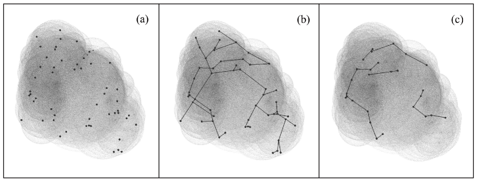
Figure 2: (a) A two-dimensional projected image of a Millennium void with dark matter halos (dots); (b) The minimal spanning tree (MST) constructed from the void halos; (c): The void mini-filaments after the MST-reduction process.

3 THE VOID FILAMENTS IN A $\Lambda$CDM UNIVERSE

We employ the filament-finding algorithm of Barrow et al. (1985) that is based on the minimal spanning tree (MST) scheme to extract the intrinsic linear patterns from the spatial distribution of the halos in the selected large voids which contain more than $30$ halos. There are three key concepts for the MST scheme: node, edge and k-branch. A node means the point (i.e., halo), an edge means a straight line that connects two nodes, and a k-branch means a path consisting of k-edges with a leaf node only at one end. That is, one end of a k-branch is free while the other end is an intersection of the edges. The MST of $N$ data points represents a unique network connected by $N-1$ edges of minimum total length without containing a closed loop.

To construct MSTs from the spatial distribution of the void halos, we follow the simplest Prim process: First, an arbitrary node (halo) is chosen as a starting point. Then the starting point is connected to its nearest neighbor along a straight line (edge). The edge composed of two nodes represents the first partial tree. The next nearest node is determined and added to the partial tree with an edge, via which the partial tree is extended. After all nodes are connected to the tree according to the above prescription, the MST construction is completed. The dominant linear patterns, i.e. filaments, are now extracted from the MSTs by taking the following MST-reduction steps (Barrow et al., 1985):

1. Pruning: An MST is pruned to the p level by eliminating all the k-branches with k$\leqslant$p.

2. Separating: All the edges longer than a given cut-off length $l_{c}$ are removed.

The Pruning process allows us to find the main stems, removing the minor twigs that hardly contribute to the main structural patterns. In other words, the superfluous small-scale noises from the MSTs are minimized and the prominent filamentary patterns are highlighted by the Pruning process. On the other hand, the Separating process breaks apart the MSTs into distinct pieces, cutting off unphysical long linkages. Both the pruning level $p$ and the cut-off length $l_{c}$ quantify the degree of the MST-reduction.

In most of the previous works where the large-scale filaments were the targets to find by means of the MST technique, the values of $p$ and $l_{c}$ were empirically determined as $p=9$ or $10$ (Barrow et al., 1985; Bhavsar & Ling, 1988a, b) and $l_{c}=f\bar{l}$ (Barrow et al., 1985; Bhavsar & Ling, 1988b; Plionis et al., 1992; Pearson & Coles, 1995; Krzewina & Saslaw, 1996; Coles et al., 1998) where $\bar{l}$ is the mean edge-length of the unreduced tree. And there were some authors who preferred $l_{c}=\bar{l}+2\sigma_{l}$ or $l_{c}=\bar{l}+\sigma_{l}$ (Bhavsar & Ling, 1988a; Zucca et al., 1991). Unlike the previous works, however, our target is not the large-scale filaments but the mini-filaments in void regions. Accordingly, the relevant values of $p$ and $l_{c}$ are supposed to be different in our case. As a practical strategy to determine the values of $p$ and $l_{c}$ for the void filaments, we investigate how the final result (i.e., the size distribution of void filaments) changes with $p$ and $l_{c}$ and look for those values at which the final result stabilizes.

With the help of this strategy, we set $p=4$ and $l_{c}=\bar{l}+\sigma_{l}$ for the void filaments. Here, the range of $p$ is obtained empirically from the distribution of k values of the unreduced trees. By setting $p=4$, we use only those branches which consist of at least $5$ edges as the main stems among the k-branches. The detailed justification of $p=4$ is given in §4. As for $l_{c}=\bar{l}+\sigma_{l}$, we examine plenty of the Millennium voids and find that the Millennium void halos have maximum number of branches when $l_{c}=\bar{l}+\sigma_{l}$ (Graham et al., 1995; Bastian et al., 2007).

Figure 3: Number distribution of void filaments as a function of the linearity, $R_{L}$ at $z=0,\ 0.5,\ 1,$ and $2$ as solid, dashed, dot-dashed, and dotted line, respectively, with single edges included (left) and excluded (right).

After completing the MST-reduction process, we end up with a final sample of the void filaments (reduced branches) with more than one edges. Fig. 2 depicts the spatial distribution of the mini-filaments in a Millennium void on a two dimensional projected plane. Table 2 lists the statistical properties of the void-filaments. Here, the linearity of a filament, $R_{L}$, is defined by the ratio of the straight distance between the two end nodes of the filament (end-to-end separation) to the sum of the lengths of all the edges constituting the filament (Barrow et al., 1985). Basically, it represents the degree of the straightness of a filament: The closer to unity the value of $R_{L}$ is, the more straight a given filament is.

Table 2: The total number of voids with more than $30$ halos ($N_{v}$), the total number of void filaments ($N_{f}$), the range of the filament numbers per a void ($n_{\rm max}$), the mean number of filaments per a void ($\bar{n}_{f}$), the mean length of void filaments ($\bar{R}_{f}$) in unit of $h^{-1}$Mpc, and the mean linearity of void filaments ($\bar{R}_{L}$) at $z=0,\ 0.5,\ 1,$ and $2$.

$z$	$N_{v}$	$N_{f}$	$n_{f}$	$\bar{n}_{f}$	$\bar{R}_{f}$	$\bar{R}_{L}$
					$[h^{-1}$Mpc]
$0$	$5604$	$22697$	$[1,22]$	$4$	$15.06$	$0.72$
$0.5$	$5992$	$24130$	$[1,16]$	$4$	$14.79$	$0.72$
$1$	$6039$	$24095$	$[1,16]$	$4$	$14.69$	$0.72$
$2$	$5349$	$20514$	$[1,16]$	$4$	$15.11$	$0.71$

Figure 3 plots the number distribution of void filaments, $N_{f}(R_{L};z)$ vs. the linearity $R_{L}$ at $z=0,\ 0.5,\ 1$ and $2$ as solid, dashed, dot-dashed, and dotted histogram, respectively, with single-edge filaments included (left) and excluded (right). As can be seen, when the single-edge filaments are included, the distribution has a peak around unity. In contrast, when the single-edge filaments are excluded, the peak occurs at $R_{L}=0.63$ and the mean linearity is reduced to $\bar{R}_{L}=0.64$. This indicates that except for the single-edge filaments most of the void filaments are not straight but curved. It can be readily understood since the void filaments are usually located in the boundary of voids.

Figure 4 plots the number distribution of voids, $N_{v}(N_{f};z)$, as a function of the number of member filaments, $N_{f}$, at $z=0,\ 0.5,\ 1$ and $2$ as solid, dashed, dot-dashed, and dotted histogram, respectively. Most of the voids have less than $10$ member filaments.

Figure 4: Number distribution of voids as a function of the number of their member filaments at $z=0,\ 0.5,\ 1,$ and $2$ as solid, dashed, dot-dashed, and dotted line, respectively.

4 THE SIZE DISTRIBUTION OF VOID MINI-FILAMENTS

We first adopt the definition of Colberg (2007) for the filament size, $S$, and measure $S$ of a given filament as the length of the diagonal line of a cuboid that exactly fits the spatial extent of the filament nodes. Let $\left(x_{\min},x_{\max}\right)$, $\left(y_{\min},y_{\max}\right)$, and $\left(z_{\min},z_{\max}\right)$ represent the full ranges of the x, y and z positions of the filament nodes, respectively. Then, $S$ is determined as

$$S=\sqrt{\left({x_{\max}-x_{\min}}\right)^{2}+\left({y_{\max}-y_{\min}}\right)^{2}+\left({z_{\max}-z_{\min}}\right)^{2}}.$$ (1)

By equation (1), we measure the size of every void filament and determine the number density of void filaments as a function of $\log S$. Fig. 5 plots the size distribution of void filaments, $dN/d\log S$, for the six different cases of the pruning level $p$ at $z=0,\ 0.5,\ 1$, and $2$ (solid, dashed, dot-dashed, and dotted line, respectively).

Figure 5: Number density of void-filaments per unit volume in a logarithmic size bin for the six different cases of the pruning level, $p$ at $z=0,\ 0.5,\ 1$ and $2$ (solid, dashed, dot-dashed, and dotted line, respectively).

When $p$ increases from $1$ to $3$, there are noticeable changes in the shape of $dN/d\log S$. Whereas, when $p$ increases from $4$ to $6$, there is only little change in the shape of $dN/d\log S$. It indicates that the onset of the stabilization of $dN/d\log S$ occurs at $p=4$. No branches are further pruned and thus the main structures of the MSTs are retained after $p=4$. This trend justifies our choice of the pruning level $p=4$ in §3. As can be seen in Fig. 5, the distribution $dN/d\log S$ appears insensitive to $z$. The four lines in each panel behave very similarly, which implies that it may be possible to express $dN/d\log S$ in a universal form. Given the fact that the sizes of the void filaments depend on the sizes of their host voids, we use the rescaled filament size, $\nu\equiv S/R_{v}$ where $R_{v}$ is the effective comoving radius of a host void that is calculated by means of the Monte Carlo integration method as described in HV02 (see also Park & Lee, 2007b).

It is found that the rescaled size distribution of void filaments $dN/d\log\nu$ at all redshifts can be well fitted to the following analytic formula:

$$f(\nu)=A\nu\exp\left({-B\nu^{2}}\right).$$ (2)

where $A$ and $B$ are the fitting parameters whose best-fit values are found through the $\chi^{2}$-minimization. Fig. 6 plots the rescaled size distributions of void filaments at four redshifts and compares them with the analytic fitting formula with the best-fit parameters. As can be seen, the numerical results at four redshifts are indeed in good agreement with the fitting model.

Yet, a careful reader may well suspect that the universality and the functional form of $dN/d\log\nu$ may depend on the definition of the filament size. To test how the fitting model and the behavior of $dN/d\log\nu$ changes with the definition of the filament size, we redefine the size of a filament as its total length, $S_{T}$, (the sum of the lengths of all edges that constitute the filament) and repeat the whole process. It is found that $dN/d\log\nu$ is still almost universal but the functional form of the fitting model is different.

$$f(\nu)=A\nu\exp\left(-B\nu\right).$$ (3)

Fig. 7 plots the same as in Fig. 6 but for the case that the filament size is measured as the total length, $S_{T}$. As can be seen, in this case $dN/d\log\nu$ decreases less rapidly. It is because the total length of a given filament is usually longer than its spatial extent. The more convoluted a filament is, the larger the difference between $S_{T}$ and $S$ is.

To make a more quantitative test of the universality of $dN/d\log\nu$, we conduct a $\chi^{2}$-statistics. Assuming the numerical result of $dN/d\log\nu$ at each redshift as one independent realization, we calculate the one standard deviation of $dN/d\log\nu$ between the four realizations, $\sigma_{j}$. One scatter error $\sigma$ in the measurement of universal value is calculated as $\sigma\equiv\sqrt{\sigma^{2}_{j}+\sigma^{2}_{p}}$ where $\sigma^{2}_{p}$ denotes the Poisson errors. With this error at each bin, we evaluate the reduced $\chi^{2}$, $\chi^{2}_{r}\equiv\chi^{2}/n_{\rm f}$ ($n_{\rm f}$: the degree of freedogm) averaged over all size bins. The values of $\chi^{2}_{r}$ are listed in Table 3 where the best-fit values of $A$ and $B$ can be also found for the cases of two different definitions of $S$. As can be seen, the values of $\chi^{2}$ are reasonably close to unity, which proves that the rescaled size distribution of void filaments is almost universal. But, it is worth noting that when the filament size is defined as the spatial extent, the distribution is more insensitive to redshift.

Figure 6: Number density of void filaments as a function of the rescaled size at $z=0,\ 0.5,\ 1$ and $2$ (open circles, squares, triangles, and diamonds, respectively). The solid line represents a fitting function (eq.[2]) with the best-fit values of $A$ and $B$. The filament size is measured as the spatial extent of the filament nodes.

Figure 7: Same as Fig.6, but the sizes of void filaments are measured as the sum of the lengths of all edges that constitute the filaments, $S_{T}$.

Table 3: The results of the reduced $\chi^{2}$ test for the size distribution of void filaments for the two different cases of the filament-size definition.

size	$A$	$B$	$\chi^{2}$
spatial extent	$0.00127$	$0.569$	$1.71$
total length	$0.00123$	$0.859$	$2.05$

5 DISCUSSION

It is generally thought that the large scale structure of the universe provides a window on the initial condition of the early universe. In previous cosmological studies, it was the halo mass function that has been most highlighted as a statistical tool for probing cosmology with the large scale structure (Press & Schechter, 1974; Sheth & Tormen, 1999; Sheth et al., 2001; Jenkins et al., 2001; Reed et al., 2003). The most advantageous aspect of the halo mass function is that it can be written in a simple universal form, independent of redshift (Sheth & Tormen, 1999). Yet, the halo mass function has a generic weakness as a cosmological probe: its dependence on the cosmological parameters comes indirectly from the dependence of the halo mass on the rms fluctuation, $\sigma(R)$, of the linear density field smoothed on a scale radius of $R$.

It is desirable to develop another statistical tool which can overcome the weakness of the halo mass function. Recently, several authors have noted the possibility of probing cosmology with cosmic voids (e.g., Sheth & van de Weygaert, 2004; Park & Lee, 2007a; Platen et al., 2008). Yet, no new statistical tool that can really compete with the halo mass function has been suggested so far. For instance, in our previous work (Park & Lee, 2007a), we have proposed that the cosmic voids provide another window on cosmology. Given that the void ellipticities are induced by the primordial tidal effect which depends on the background cosmology, we have shown analytically that the void ellipticity distribution can be used to constrain the cosmological parameters.

However, it has turned out that the void ellipticity distribution suffers from the same weakness that the halo mass function has. Its dependence on cosmology is secondary, resulting from the dependence of the void scale on the linear rms density fluctuation, $\sigma(R)$. Furthermore, the void ellipticity distribution cannot be written in a universal form unlike the halo mass function. Therefore, true as it is that the void ellipticity distribution provides another way to determine the cosmological parameters with the large scale structure, it is not competitively compared with the halo mass function.

In this work, we have for the first time quantified the effect of the tidal field on cosmic voids by the sizes of the void filaments. It is shown that the size distribution of void filaments is almost independent of redshift, having a simple universal form. A crucial implication of our result is that the number density of long filaments in voids should depend very sensitively on the background cosmology since the sizes of the void filaments reflect the primordial tidal field.

Our result that the size distribution of void filaments is almost independent of redshift in spite of the well known fact that the sizes of voids grow very strongly with redshift can be understood as follows. It is true that the comoving sizes of voids keep growing as the voids expand faster than the rest of universe due to their extreme low density. However, the comoving sizes of void filaments should not necessarily keep growing with redshift.

But for the effect of the tidal field, the spatial distribution of void halos would be isotropic due to the gravitational rarefaction effect caused by the fast expansion of voids. In other words, while the gravitational rarefaction effect tends to make the spatial distribution of void halos isotropic, the tidal effect on voids tends to increase the anisotropy in the distribution of void halos, resulting in growth of void filaments. Therefore, as far as the tidal effect exists and counteracts the expansion effect, the sizes of void filaments will also grow as the sizes of their host voids grow with redshift.

However, when the void size grows large enough to finally reach its threshold at which the expansion effect overcomes the tidal effect, the degree of anisotropy in the spatial distribution of void halos will diminish and accordingly the sizes of void filaments will stop growing. Since this critical threshold of void size is determined by the single condition that the expansion effect overcomes the tidal effect, its value should be redshift-independent. At high-redshift when the sizes of voids were small, the strong dominant tidal effect increases the anisotropy in the spatial distribution of void halos, increasing the sizes of void filaments. At low-redshift when the sizes of voids are large, the strong expansion effect prevents the sizes of void filaments from keep growing. Hence, the universal size distribution of void filaments reflects the fact that the sizes of void filaments are regulated by the counter-balance between the expansion effect and the tidal effect.

The fitting formula, eqs. (2)-(3), indicate that the number density of void filaments, $dN/d\log\nu$, behaves like a power-law with power index of $n=1$ in the short filament section while it decreases exponentially in the long filament section. A crucial implication of our result is that the exponential decrease of the abundance of long-size filaments in voids should be very sensitive to the key cosmological parameters. Especially it is expected to depend sensitively on the amplitude of the linear power spectrum, $\sigma_{8}$. In our previous work, we have already shown that the void ellipticity caused by the tidal effect increases with the value of $\sigma_{8}$ (Park & Lee, 2007a). Accordingly, we expect that the number density of long filaments in voids would increase as the value of $\sigma_{8}$ increases. Unlike the void ellipticity distribution whose dependence on $\sigma_{8}$ is weak and indirect through its dependence on the rms density fluctuation, equation (2) suggests that the size distribution of void filaments should depend strongly on the power spectrum amplitude.

To use the size distribution of void filaments as a cosmological probe, however, there should be some additional tasks to be done in the future. First, the mass-to-light bias and the redshift distortion effects have to be account for. What one can observe is not halos in real space but galaxies in redshift space. The size distribution of void filaments measured from the galaxy catalogs in redshift space could differ from the current result. Thus, it will be very necessary to investigate how the bias and the redshift distortion effect change the size distribution of void filaments. It is expected that the sizes of void filaments may increase in redshift space since the redshift space distortion effect tend to increase the anisotropy in the spatial distribution of void galaxies. Meanwhile, the matter-to-light bias might decrease the sizes of void filaments, compensating for the redshift distortion effect, since the massive halos are found to be distributed less anisotropically (Park & Lee 2009 in preparation). Henceforth, the overall size distribution of void galaxy filaments in redshift space might be similar to that in real space, due to the competition between the two effects (in private communication with van de Weygaert).

Second, a general analytic formula for the size distribution of void filaments in an arbitrary cosmology is desirable to derive from physical principles. If an analytic model is found, it would allow us to understand the true physical meaning of eqs. (2)-(3). Third, it should be worth examining whether the results depend on the choice of the filament-finding and the void-finding algorithms. As mentioned in §1, it has been found that different void-finders provide different void properties and the HV02 algorithm that we used here has a tendency to find larger voids than most of the other void-finders (Colberg et al., 2008). Furthermore, our results are not general ones but valid only for the specific cosmology of the Millennium Run simulation. Therefore, it is required to test the universality of the size distribution of void filaments with other void-finders and with other cosmologies as well. We plan to address these issues and report the results elsewhere in the near future.

References

- Aragón-Calvo et al. (2007) Aragón-Calvo, M. A., Jones, B. J. T., van de Weygaert, R., & van der Hulst, J. M., 2007, A& A, 474, 315
- Barrow et al. (1985) Barrow, J. D., Bhavsar, S. P., & Sonoda, D. H., 1985, MNRAS, 216, 17
- Bastian et al. (2007) Bastian, N., Ercolano, B., Gieles, M., Rosolowsky, E., Scheepmaker, R. A., Gutermuth, R., & Efremov, Yu., 2007,MNRAS, 379, 1302
- Bhavsar & Ling (1988a) Bhavsar, S. P., & Ling, E. N., 1988a, ApJL, 331, 63
- Bhavsar & Ling (1988b) Bhavsar, S. P., & Ling, E. N., 1988b, PASP, 100, 1314
- Bond et al. (1996) Bond, J., R., Kofman, L., & Pogosyan, D., 1996, Nature, 380, 603
- Colberg (2007) Colberg, J. M., 2007, MNRAS, 375, 337
- Colberg et al. (2008) Colberg, J. M. et al., 2008, MNRAS, 387, 933
- Coles et al. (1998) Coles, P., Pearson, R. C., Borgani, S., Plionis, M., & Moscardini, L., 1998, MNRAS, 294, 245
- Colless et al. (2001) Colless et al., 2001, MNRAS, 328, 1039
- Einasto (2006) Einasto, J., 2006, Formation of the Supercluster-Void Networks, proceedings of the Detre Centennial Conference : Communications from the Konkoly Observatory, ed. L.-G. Balazs, L. Szabados, A. Holl (CoKon Homepage), 104
- El-Ad & Piran (1997) El-Ad, H., & Piran, T., 1997, ApJ, 491, 421
- Graham et al. (1995) Graham, M. J., Clowes, R. G., & Campusano, L. E., 1995, MNRAS, 275, 790
- Hahn et al. (2007) Hahn, O., Carollo, C. M., Porciani, C., & Dekel, A., 2007, MNRAS, 381, 41
- Hoyle & Vogeley (2002) Hoyle, F., & Vogeley, M. S., 2002, ApJ, 566, 641
- Jenkins et al. (2001) Jenkins, A., Frenk, C. S., White, S. D. M., Colberg, J. M., Cole, S., Evrard, A. E., Couchman, H. M. P., & Yoshida, N., 2001, MNRAS, 321, 372
- Krzewina & Saslaw (1996) Krzewina, L. G., & Saslaw, W. C., 1996, MNRAS, 278, 869
- Lee & Evrard (2007) Lee, J., & Evrard, A. E., 2007, ApJ, 657, 30
- Lee & Park (2006) Lee, J., & Park, C., 2006, ApJ, 662, 1
- Park et al. (2007) Park, C., Choi, Y.-Y., Vogeley, M. S., Gott, J. R. I., & Blanton, M. R., 2007, ApJ, 658, 898
- Park & Lee (2007a) Park, D., & Lee, J., 2007, Phys. Rev. Lett., 98, 081301
- Park & Lee (2007b) Park, D., & Lee, J., 2007, ApJ, 665, 96
- Pearson & Coles (1995) Pearson, R. C., & Coles, P., 1995, MNRAS, 272, 231
- Peebles (2001) Peebles, P. J. E., 2001, ApJ, 557, 495
- Platen et al. (2008) Platen, E., van de Weygaert, R., & Jones, B. J. T., 2008, MNRAS, 387, 128
- Plionis et al. (1992) Plionis, M., Valdarnini, R., & Jing, Y. P., 1992, ApJ, 398, 12
- Press & Schechter (1974) Press, W., & Schechter, P., 1974, ApJ, 187, 425
- Reed et al. (2003) Reed, D., Gardner, J., Quinn, T., Stadel, J., Fardal, M., Lake, G., & Governato, F., 2003, ApJ, 379, 440
- Sahni et al. (1994) Sahni, V., Sathyaprakash, B. S., & Shandarin, S. F., 1994, ApJ, 431, 20
- Sahni & Shandarin (1996) Sahni, V., & Shandarin, S. F., 1996, MNRAS, 282, 641
- Shandarin et al. (2004) Shandarin, S. F., Sheth, J. V., & Sahni, V., 2004, MNRAS, 353, 162
- Shandarin et al. (2006) Shandarin, S., Feldman, H. A., Heitmann, K., & Habib, S., 2006, MNRAS, 367, 1629
- Sheth & Tormen (1999) Sheth, R. K., & Tormen, G., 1999, MNRAS, 308, 119
- Sheth et al. (2001) Sheth, R. K., Mo, H. J., & Tormen, G., 2001, MNRAS, 323, 1
- Sheth & van de Weygaert (2004) Sheth, R. K., & van de Weygaert, R., 2004, MNRAS, 350, 517
- Springel et al. (2005) Springel, V. et al., 2005, Nature , 435, 629
- Zucca et al. (1991) Zucca, E., Bardelli, S., Cappi, A., & Moscardini, L., 1991, MNRAS, 253, 401